HAL Id: hal-01329051
https://hal.archives-ouvertes.fr/hal-01329051
Submitted on 8 Jun 2016
HAL is a multi-disciplinary open access
archive for the deposit and dissemination of
sci-entific research documents, whether they are
pub-lished or not. The documents may come from
teaching and research institutions in France or
abroad, or from public or private research centers.
L’archive ouverte pluridisciplinaire HAL, est
destinée au dépôt et à la diffusion de documents
scientifiques de niveau recherche, publiés ou non,
émanant des établissements d’enseignement et de
recherche français ou étrangers, des laboratoires
publics ou privés.
The best of both worlds: synthesis-based acceleration
for physics-driven cosparse regularization
Srdan Kitic, Nancy Bertin, Rémi Gribonval
To cite this version:
Srdan Kitic, Nancy Bertin, Rémi Gribonval. The best of both worlds: synthesis-based acceleration for
physics-driven cosparse regularization. iTwist 2016 - International Traveling Workshop on Interactions
Between Sparse Models and Technology, Aug 2016, Aalborg, Denmark. �hal-01329051�
The best of both worlds: synthesis-based acceleration
for physics-driven cosparse regularization
Sr ¯
dan Kiti´c
1, Nancy Bertin
2and Rémi Gribonval
3.
1Technicolor R&D,2CNRS - UMR 6074,3Inria, France.∗
Abstract— Recently, a regularization framework for ill-posed inverse problems governed by linear partial differential equa-tions has been proposed. Despite nominal equivalence between sparse synthesis and sparse analysis regularization in this con-text, it was argued that the latter is preferable from computational point of view (especially for huge scale optimization problems aris-ing in physics-driven settaris-ings). However, the synthesis-based opti-mization benefits from simple, but effective all-zero initialization, which is not straightforwardly applicable in the analysis case. In this work we propose a multiscale strategy that aims at exploiting computational advantages of both regularization approaches.
1
Introduction
Linear partial differential equations (pde) are ubiquitous in mathematical models of physical laws. Hence, whether in im-plicit or exim-plicit form, they appear in various signal processing inverse problems (ranging from, e.g. sound source localiza-tion to brain imaging). Inspired by impressive results in sparse signal recovery and compressed sensing [1], several works e.g. [2, 3, 4, 5, 6] have proposed an explicit use of such physical models in regularization of some highly ill-posed inverse prob-lems (baptized “physics-driven” regularization methods).
Generally, a linear pde models the relation among two phys-ical quantities (x, z) as Ax = z, where the linear operator A encapsulates the pde with appropriate initial and/or boundary conditions. Analogously, one can write x = Dz, where D is a linear operator acting as an “inverse” to A. Particularly, D is the integral operator encoding the so-called Green’s functions, i.e. impulse responses of the operator A. One is interested in inferring the quantity z, which is often characterized by a small number of free parameters (representing, for instance, domi-nant sources of brain activity in an EEG application). On the other hand, we are only given a few measurements y of the quantity x (e.g. voltage measurements at the surface of the head). The measurements are, therefore, acquired by apply-ing a subsamplapply-ing operator M to the signal x. This problem is severely ill-posed, and one way of addressing it is by asking for an estimate ˆz (analogously, Aˆx) having the lowest complexity, i.e.the fewest degrees of freedom possible.
Analytical solutions of pdes are available only in certain re-stricted regimes. In other cases, one approaches the problem numerically and discretizes the involved quantities and opera-tors (A → A ∈ Rn×n, x → x ∈ Rn, D → D ∈ Rn×n,
z → z ∈ Rn, M → M ∈ Rm×n, y → y ∈ Rm). It should be clear that D = A−1, which is identical to computing the response of a linear system defined by A for an impulse placed at every point of a discrete n-dimensional domain.
∗This work was supported in part by the European Research Council,
PLEASE project (ERC-StG-2011-277906).
Low complexity can be promoted through sparsity [1] of z (minimizing kzk0) or cosparsity [7] of x (minimizing kAxk0).
A common relaxation to these problems is the constrained `1
norm minimization (a.k.a. basis pursuit), either in the sparse analysis
minimize
x kAxk1 subject to Mx = y, (1)
or sparse synthesis flavor minimize
z kzk1subject to MDz = y. (2)
The pde-encoding matrix A thus represents the analysis oper-ator, while the row-reduced Green’s function-encoding matrix MD represents the (synthesis) dictionary.
2
The Chambolle-Pock algorithm
A popular method for solving large scale nonsmooth problems such as (1) and (2) is the so-called Chambolle-Pock or precon-ditioned ADMM algorithm [8]. It is a primal-dual approach based on the saddle point interpretation of the original con-strained problem. Iteratively solving intermediate primal and dual problems avoids matrix inversion, hence its per-iteration cost is dominated by the cost of evaluating matrix-vector prod-ucts and proximal operators. To make the latter efficient, one needs to appropriately customize the saddle-point problem to leverage all available structures.
Particularly, in the analysis case, we exploit the fact that M is a row-reduced identity matrix. This allows for cheap projection to a set Θ = {x | Mx = y}, leading to the following saddle point formulation:
minimize
x maximizeλ hAx, λi + χΘ(x) − ` ∗
1(λ), (3)
where χΘ is the indicator function of the set Θ and `∗1 is the
convex conjugate [9, 11] of the `1norm function (i.e. an
indi-cator function of the `∞ball). In the synthesis case, we exploit
the separability of the kzk1objective, which yields the standard
Lagrangian problem: minimize
z maximizeλ hMDz − y, λi + `1(z). (4)
In both cases, λ represents the corresponding dual variable. The Chambolle-Pock algorithm essentially evaluates two proximal operators per iteration, each assigned to primal and dual variable, respectively. For the presented problems, the al-gorithm is actually (asymptotically) first-order optimal, since it obtains O(1/k) convergence rate1 [8, 10] when all penalties
are non-smooth, but structured [11]. More precisely, decrease of the primal-dual gap is proportional to kAk22/k, in the analy-sis, and to kMDk22/k, in the synthesis case (k · k2denotes the
induced 2-norm of a matrix).
3
Computational differences
Assuming that the regularization indeed yields well-posed problems, solving (1) or (2) is equivalent, in the sense that using the solution of one problem, we can easily recover the solution of another (since Ax = z). However, as demonstrated in [12], the two optimization problems significantly differ from com-putational point of view. In fact, if the applied discretization is locally supported (which is often the case with, e.g., finite difference or finite element discretization methods), the anal-ysis operator A is extremely sparse (with O(n) nonzero en-tries), while the dictionary MD is most often a dense matrix (O(mn)). But the differences do not end there: as widely rec-ognized [13], physical problems are often unstable, since small changes in z can induce large fluctuations of x. In line with that, discretization usually leads to increasingly ill-conditioned systems: the condition number κ = σmax/σminof A (eq. D)
grows fast with n. However, one can often factorize the anal-ysis operator (with abuse of notation) as τ A, where the scale factor τ depends only on the discretization stepsize and the en-tries of A remain constant (this will be validated on the actual example in the following section). Notice that, in the basis pur-suit problem (1), the scale τ does not affect the solution, and can be neglected. Now, the growth of κ is due to decrease of the smallest singular value of A (i.e. increase of the largest sin-gular value of D = A−1), hence σmax(A) = kAk2is stable.
The consequence for the primal-dual algorithm discussed previously, is that (at worst) the synthesis approach will require orders of magnitude more iterations to converge, in addition to high computational cost per iteration. Given these arguments, one may conclude that it should be completely avoided in the physics-driven context. However, it has an important advantage over the analysis-based optimization: since the expected solu-tion is sparse, a simple all-zero initial estimate is already close to the optimal point. In order to exploit this feature, we propose a simple scheme: i) apply crude (low-resolution) discretization, and solve the problem (4) to obtain the crude estimate ˜x = D˜z; ii) interpolate ˜x to a target high-resolution discretization and use it as an initial point ˆx(0)for the problem (3).
4
An example: 1D Laplacian
We will demonstrate the idea on a simple one-dimensional problem. Assume that on a domain r ∈ [0, φ], a physical pro-cess is modeled as
d2x(r)
dr2 = z(r), (5)
with x(0) = x(φ) = 0 (e.g. modeling a potential distribution of a grounded thin rod, with sparse “charges” z(r)).
By applying the second order finite difference discretization to this problem, we end up with a well-known symmetric tridi-agonal Toeplitz matrix A (i.e. 1D discrete Laplacian), with a “stencil” defined as τ [−1, 2, −1] (henceforth, we neglect τ ). This simple matrix allows for fast computation of A−1z using the Thomas algorithm [14]. In addition, it admits simple an-alytical expressions for extremal singular values [15], namely σmax = 2 − 2 cos(n+1nπ ), and σmin = 2 − 2 cos(n+1π ). The
ill-conditioning with regards to the size n is obvious, but the true value of kMDk2 is somewhat lower than 1/σmin, since
it also depends on the number of measurements m and the re-alization of the presumed random sampling. In general, one expects kMDk2→ 1/σminas m → n.
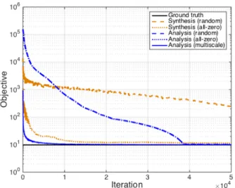
Figure 1:“Objective” := ksk1+ krk22, where s is a sparse estimate
(e.g. Ax) and r is a residual vector (e.g. Mx − y).
To verify our claims, we simulated the problem of size n = 103, with the size of the support set being kzk
0= 10
(cho-sen uniformly at random from the set [1, n], with coefficients iid distributed as N (0, 1)). The measurement vector y contains (selected uniformly at random) m = 250 samples of the signal x = A−1z. The iteration threshold is set to kmax= 5 × 10⁴.
We first solve both problems (1) and (2) (using the appro-priate versions of the Chambolle-Pock algorithm), by generat-ing the initial points ˆx(0)and ˆz(0)randomly (iid sampled from N (0, 1)), and then re-running both versions with all-zero ini-tialization. Objective function decrease graphs in Figure 1 con-firm our findings: when both algorithms are randomly initial-ized, the analysis one exhibits considerably faster convergence (moreover, the synthesis version does not reach the ground truth value). However, when the synthesis algorithm is initialized with an all-zero vector, it converges rapidly, outperforming the analysis approach in both cases (for which, interestingly, the two initializations yield the same convergence curve).
Unfortunately, in practice we are rarely capable of efficiently applying the synthesis approach, since cheap computation of A−1z is possible only in specific cases. Otherwise, MD needs to be explicitly computed and stored, leading to memory bot-tlenecks and high per-iteration cost. To alleviate this issue, we exploit the aforementioned multiscale strategy. First, the syn-thesis version is appropriately initialized (with an all-zero vec-tor) and solved on a crude, nlow = 500 grid. Then its
spline-interpolated (cf. [15]) estimate is used to initialize the full reso-lution analysis-based solver. The “analysis (multiscale)” graph presented in Figure 1 verifies that this scheme is indeed very ef-ficient, in this case converging the fastest among all considered algorithms and initializations.
5
Conclusion
We have presented a simple, yet effective acceleration of the analysis-based optimization, in the physics-driven set-ting. Leveraging the synthesis-based initialization enables or-ders of magnitude faster convergence compared to the naive case. Even though only a simple 1D Laplacian case was dis-cussed and justified, we feel that the same methodology holds in more involved scenarios, comprising different multidimen-sional pdes with complicated boundary conditions.
References
[1] S. Foucart and H. Rauhut, “A mathematical introduction to compressive sensing”, Springer, 1(3), 2013.
[2] D. Malioutov, M. Çetin and A. S. Willsky, “A sparse sig-nal reconstruction perspective for source localization with sensor arrays”, IEEE Transactions on Signal Processing, 53(8):3010–3022, 2005.
[3] L. Stenbacka, S. Vanni, K. Uutela and R. Hari, “Compar-ison of minimum current estimate and dipole modeling in the analysis of simulated activity in the human visual cortices”, NeuroImage, 16(4): 936–943, 2002.
[4] I. Dokmani´c and M. Vetterli, “Room helps: Acoustic localization with finite elements”, IEEE International Conference on Acoustics, Speech and Signal Processing (ICASSP): 2617–2620, 2012.
[5] S. Nam and R. Gribonval, “Physics-driven structured cosparse modeling for source localization”, IEEE Interna-tional Conference on Acoustics, Speech and Signal Pro-cessing (ICASSP): 5397–5400, 2012.
[6] J. Murray-Bruce and P. L. Dragotti, “Spatio-temporal sampling and reconstruction of diffusion fields induced by point sources”, IEEE International Conference on Acoustics, Speech and Signal Processing (ICASSP): 31– 35, 2014.
[7] S. Nam, M. E. Davies, M. Elad and R. Gribonval, “The cosparse analysis model and algorithms”, Applied and Computational Harmonic Analysis, 34(1):30–56, 2013. [8] A. Chambolle and T. Pock, “A first-order primdual
al-gorithm for convex problems with applications to imag-ing”, Journal of Mathematical Imaging and Vision, 40(1): 120–145, 2011.
[9] S. Boyd and L. Vandenberghe, “Convex optimization”, Cambridge university press, 2004.
[10] A. Chambolle and T. Pock, “On the ergodic convergence rates of a first-order primal–dual algorithm”, Mathemati-cal Programming (Springer): 1–35, 2015.
[11] Y. Nesterov, “Introductory lectures on convex optimiza-tion: A basic course”, Springer Science & Business Me-dia, 87, 2013.
[12] S. Kiti´c, L. Albera, N. Bertin and R. Gribonval, “Physics-driven inverse problems made tractable with cosparse reg-ularization”, IEEE Transactions on Signal Processing, 64(2): 335–348, 2016.
[13] V. Isakov, “Inverse problems for partial differential equa-tions”, Springer Science & Business Media, 127, 2006. [14] L. H. Thomas, “Using a computer to solve problems
in physics”, Applications of Digital Computers (Boston: Ginn and Company): 44–45, 1963.
[15] G. Strang, “Computational science and engineering”, Wellesley-Cambridge Press Wellesley, 1, 2007.