Blind Harmonic Adaptive Decomposition Applied to Supervised Source Separation

HAL Id: hal-00945288

https://hal.inria.fr/hal-00945288

Submitted on 24 Mar 2014

HAL is a multi-disciplinary open access

archive for the deposit and dissemination of

sci-entific research documents, whether they are

pub-lished or not. The documents may come from

teaching and research institutions in France or

abroad, or from public or private research centers.

L’archive ouverte pluridisciplinaire HAL, est

destinée au dépôt et à la diffusion de documents

scientifiques de niveau recherche, publiés ou non,

émanant des établissements d’enseignement et de

recherche français ou étrangers, des laboratoires

publics ou privés.

Blind Harmonic Adaptive Decomposition Applied to

Supervised Source Separation

Benoît Fuentes, Roland Badeau, Gael Richard

To cite this version:

Benoît Fuentes, Roland Badeau, Gael Richard. Blind Harmonic Adaptive Decomposition Applied

to Supervised Source Separation. 20th European Signal Processing Conference (EUSIPCO), 2012,

Bucharest, Romania. pp.2654–2658. �hal-00945288�

BLIND HARMONIC ADAPTIVE DECOMPOSITION APPLIED TO SUPERVISED SOURCE

SEPARATION

Benoit Fuentes, Roland Badeau, Gaël Richard

Institut Mines-Télécom,Télécom ParisTech, CNRS LTCI

37-39, rue Dareau - 75014 Paris - France

benoit.fuentes@telecom-paristech.fr

ABSTRACT

In this paper, a new supervised source separation system is in-troduced. The Constant-Q Transform (CQT) of an audio signal is first analyzed through an algorithm called Blind Harmonic Adaptive Decomposition (BHAD). This algorithm provides an estimation of the polyphonic pitch content of the input signal, from which the user can select the notes to be extracted. The system then automatically separates the corresponding source from the audio mixture, by means of time-frequency masking of the CQT. The system has been evaluated both in a task of multipitch estimation in order to measure the quality of the decomposition, and in a task of user-guided melody extraction to assess the quality of the separation. The very promising results obtained highlight the reliability of the proposed model. Index Terms— Audio Source Separation, Harmonic De-composition, PLCA, NTF

1. INTRODUCTION

Spectrogram decomposition techniques into meaningful basic elements such as Nonnegative Matrix Factorization are now widely used to perform monaural source separation of audio mixtures [1]. However, performing this task in a completely blind way remains challenging, basically due to the difficulty of clustering the basic elements that belong to the same source. To overcome this problem, one solution is to inform the sep-aration, e.g. whether with the aligned score of the audio [2] or with user-specifiable constraints over the present sources in the mixture [3].

In this paper, another approach is followed, similar to [4], where no side information is needed (the decomposition is blindly performed) but where the user can cluster the basic elements of the sources to be separated. In fact, the proposed system allows the user choosing the notes to be extracted via an intuitive Graphical User Interface (GUI) showing an estimation of the polyphonic pitch content of the input signal. This work relies on [5], where it was proven that efficient translation-invariant models for music analysis on the CQT of an audio

The research leading to this paper was partly supported by the Quaero Programme, funded by OSEO, French State agency for innovation.

signal can be directly applied to source separation. Thus, the article is organized as follows: first, the statistical framework that is employed to model the noise and the polyphonic part of a CQT is described in section 2. We present the algorithm for estimating the model parameters in section 3. In section 4, a new sparseness prior is introduced in order to constrain the parameters to converge towards a meaningful solution. The application to source separation is explained in section 5, where the GUI is described and the separation process explained. Finally, we present two different evaluations of the method in section 6 and conclude in section 7.

2. PROBABILISTIC MODEL FOR THE INPUT CQT The framework on which the presented model relies is the Probabilistic Latent Component Analysis (PLCA) following the example of [6]. It is a probabilistic tool for non-negative data analysis which offers a convenient way of designing spec-trogram models and introducing priors on the corresponding parameters. Let us consider the absolute value of the CQT Xf tof an audio signalx, denoted Vf t= |Xf t|. In PLCA, it is

modeled as the histogram ofN independent random variables (fn, tn) ∈ Z × J1; T K, which represent time-frequency bins,

distributed according toP (f, t) (we suppose that Vf t= 0 for

f /∈ J1, F K). P (f, t) can then be parameterized according to the desired decomposition ofVf tand the parameters can

be found by means of the Expectation-Maximization (EM) algorithm. In the inherent model of the BHAD algorithm (that we call the BHAD model), a first latent variablec is intro-duced in order to decomposeVf tas a sum of a polyphonic

harmonic signal (in this case,c = h) and a noise signal (c = n) (the notationsPh(.) and Pn(.) are used for P (.|c = h) and

P (.|c = h)):

P (f, t) = P (c = h)Ph(f, t) + P (c = n)Pn(f, t), (1)

wherePh(f, t)_{(f,t)∈Z×J1,T K}andPn(f, t)_{(f,t)∈Z×J1,T K}

respec-tively represent the normalized CQTs of the polyphonic and the noise signals. The models for each component are pre-sented in the following sections.

2.1. The notes model

At a given timet, the spectrum of the polyphonic component, represented byPh(f, t), is decomposed as a weighted sum of

different harmonic notes, each one having its own fundamental frequency (on a discrete logarithmic scalepitch(i)i∈J0,I−1K)

and spectral envelope. Since the number of notes is unknown, we consider all possible fundamental frequencies, with possi-bly zero weights:

Ph(f, t) =

︁

i

Ph(i, t)Ph(f |i, t), (2)

where i ∈ J0, I − 1K is a new latent variable representing the note of fundamental frequency pitch(i). Ph(i, t) and

Ph(f |i, t) respectively represent the energy and the

normal-ized harmonic spectrum of notei at time t. Ph(i, t) can thus

be seen as time-frequency note activations.

In order to account for the harmonic nature ofPh(f |i, t),

as well as its specific spectral envelope, the same principle as in [7] is adopted. The spectrum of a harmonic note is decomposed as a weighted sum ofZ fixed narrow-band harmonic spectral kernels, denotedPh(f |z, i), sharing the same fundamental

frequencypitch(i) and having their energy concentrated at the zth_harmonic:

Ph(f |i, t) =

︁

z

Ph(z|i, t)Ph(f |z, i). (3)

The applied weights, included inPh(z|i, t), define the spectral

envelope of the current note. Working with the CQT has a main advantage, since for a harmonic note, a pitch modulation can be interpreted as a frequency shifting of the partials. Therefore, for giveni and z, Ph(f |z, i) can be deduced from a single

templatePh(µ|z)µ∈J1,F Kas follows:

Ph(f |z, i) = Ph(f − i|z). (4)

Here,Ph(µ|z) is also a narrow-band harmonic kernel, having

its energy concentrated on thezth_{harmonic. Its fundamental}

frequency ispitch(0). Its precise definition can be see in the function make_Kernel.m of the online matlab code [8]. Contrary to [9], the kernels have been designed in order to have energy only for the frequency bins corresponding to harmonics. The spectral spreading of the partials of a note is therefore not taken into account by the kernels but by the note activations, various joint values ofi being necessary to explain a single note. Doing so allows insuring that the model can fit any spectral spreading of the partials (for instance, a continuous variation of pitch induces a larger spreading at a given time).

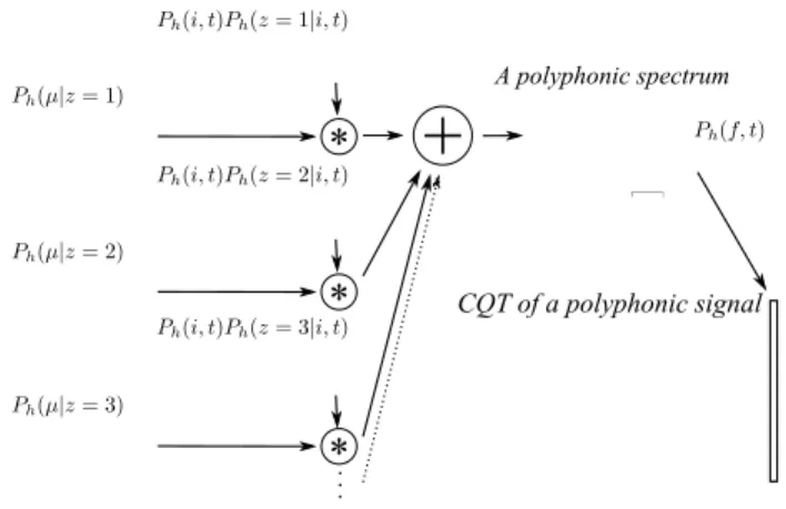
Finally, the whole polyphonic component model can be written as:

Ph(f, t) =

︁

i,z

Ph(i, t)Ph(z|i, t)Ph(f − i|z). (5)

One can notice that we end up with a convolutive model, meaning that variablef is defined as the sum of two random variablesµ and i. Fig. 1 illustrates this model.

+

*

*

*

Fig. 1. Polyphonic component of the BHAD model. At time t0, the vectorPh(i, t0) should have as many peaks as there are

active notes in the signal.

2.2. The noise model

Similarly to [7], the CQT of the noise signal is modeled as the convolution of a fixed smooth narrow-band

win-dowPn(µ)µ∈J1,F K, and a noise time-frequency distribution

Pn(i, t)(i,t)∈J0,I−1K×J1,T K:

Pn(f, t) =

︁

i

Pn(i, t)Pn(f − i). (6)

3. PARAMETERS ESTIMATION: EM ALGORITHM In [7], it is explained how to derive the EM algorithm. This algorithm defines update rules for the parameters so that the log-likelihoodL of the observations increases at every iteration (it can be proven thatL =︀

f,tVf tln (P (f, t))).

First, in the "expectation step", the posterior distribution of latent variablesi, z and c is computed by applying the Bayes’ theorem:

P (i, z,c = h|f, t) = P (c = h)Ph(i, t)P_{P (f, t)}h(z|i, t)Ph(f − i|z), (7) P (i,c = n|f, t) = P (c = n)Pn(i, t)Pn(f − i)

P (f, t) . (8) Equations (1), (5) and (6) defineP (f, t).

Then, in the "maximization step", the log-likelihood of observed and latent variablesQΛis maximized, leading to the

following updates rules: P (c = h) ∝ ︁ f,t,z,i Vf tP (i, z, c = h|f, t), (9) Ph(i, t) ∝ ︁ f,z Vf tP (i, z, c = h|f, t), (10)

Ph(z|i, t) ∝ ︁ f Vf tP (i, z, c = h|f, t), (11) P (c = n) ∝︁ i,f,t Vf tP (i, c = n|f, t), (12) Pn(i, t) ∝ ︁ f Vf tP (i, c = n|f, t). (13)

After initialization of the parameters, the EM algorithm con-sists in iterating equations (7) and (8), the different update rules (equations (9) to (13)) and finally the normalization of all parameters so that the probabilities sum to one.

4. SPARSENESS PRIOR

In practice, running the presented algorithm without any ad-ditional prior does not give relevant estimations of the param-eters. Indeed, for one note of pitchf0actually present in the

input signal, all notesi whose fundamental frequency is a multiple or a submultiple off0will be activated. Thus, even

if the log-likelihood of the data after convergence is high, the decomposition might not be informative enough. In order to overcome this flaw, we add a sparseness prior to the note acti-vationsPh(i, t), assuming it is more likely to explain the same

set of data using a fewer number of active notes.

If θ is theI × T matrix of coefficients θit= Ph(i, t), the

prior we put forward is defined as follows: P r(θ) ∝ exp︁−2β√IT ‖θ‖1/2 ︁ . (14) where‖θ‖1/2 = ︀ i,t √ θit. β is a hyperparameter defining

the strength of the prior and the coefficient√IT is such that the strength is independent of the size of the data. In Ap-pendix A, it is proven that ifβ2 _< ︀

i,twit2/(IT ), where

wit =︀_f,zVf tP (i, z, c = h|f, t), then the update rule (10)

followed by its normalization are replaced by: Ph(i, t) = 2w2 it IT β2_{+ 2ρw} it+ β √ IT︀IT β2_{+ 4ρw} i,j , (15) ρ being the unique positive number such that Ph(i, t) sums

to one. This number can be found with any root finder algo-rithm (we used the fzero Matlab function). In practiceβ is set to a sufficiently low value so thatβ2 _{is always inferior}

to︀

i,twit2/(IT ). The effect of using the sparseness prior is

illustrated in Fig. 2.

5. APPLICATION TO SUPERVISED SOURCE SEPARATION

In this section, it is explained how the BHAD model can be used to perform supervised source separation. The main idea is to provide a note selection tool where the user chooses via a GUI which notes actually present in the input file are to be separated from the rest of the audio.

0 10 20 30 −4 −3.9 −3.8 −3.7 −3.6x 10 6 Iterations Log−posterior probability 0 10 20 30 −3.7 −3.65 −3.6 −3.55 −3.5x 10 6 Iterations Log−likelihood with no prior

Time (s) P itch (MI DI scale)

Time−frequency activations using the prior

0 2 4 6 40 60 80 100 Time (s) P itch (MI DI scale)

Time−frequency activations using no prior

0 2 4 6 40 60 80 100 Time (s) Log− freq uency Input CQT 0 2 4 6 Time (s) P itch (MI DI scale)

Ground−thruth pitch activity

0 2 4 6

40 60 80 100

Fig. 2. Illustration of the use of the sparseness prior. The input signal corresponds to an excerpt from Bach’s Prelude and Fugue in D major BWV 850. The growth of the criterion over the iterations of the EM algorithm has also been plotted.

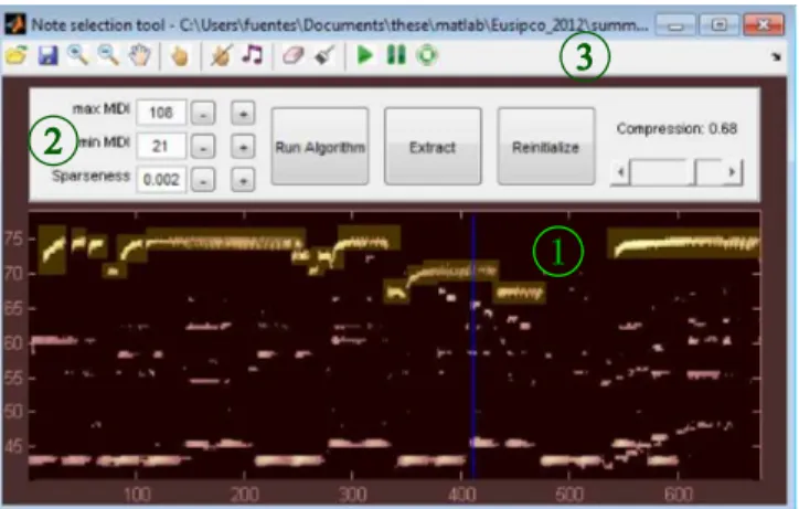
5.1. GUI and notes selection

The BHAD model offers a relevant mid-level representation of audio, since note activationsPh(i, t) indicate the active

notes with respect to time, like in a "piano-roll" representation. Using Matlab, a GUI has been developed (available at [8]), as shown in Fig. 3, where the user can highlight the notes to be extracted. The GUI consists of the following elements: (1) the representation of note activationsPh(i, t), on which the user

can select notes or edit the data (erase and draw functions) if he notices that the BHAD algorithm gave wrong estimations; (2) the control panel, where the user can set hyperparameters for the BHAD algorithm (such as the sparseness strengthβ), run the algorithm, separate the selected notes, reinitialize all parameters and change the contrast of the representation of the activations; (3) the toolbar, composed of basic tools in order to load a new wave file or a previous work, to save the current work, to explore the image, to select or unselect notes, to listen to a note whose pitch corresponds to the same pitch than the selected note, to edit the note activations and finally to listen to the signal.

5.2. Source model and time-frequency masking

The user, by highlighting the notes he wants to extract with the "select note" tool, defines a binary maskB(i, t) on the note activations, equal to1 if a time-frequency bin is selected and0 otherwise. B(i, t) can be used to perform the separation by means of time-frequency masking on the input CQT. Two masks,M1andM2, which respectively correspond to source1

1

2

3

Fig. 3. GUI of the note selection tool. The input file is an ex-cerpt from the jazz standard Summertime composed by George Gershwin. The highlighted areas correspond to notes selected by the user.

(the selected notes) and source2 (the residual), are defined as:

M1(f, t) =

P (c = h)︀

i,zB1(i, t)Ph(z|i, t)Ph(f − i|z)

P (f, t) , (16) M2(f, t) = 1 P (f, t) ︁ P (c = n)Pn(f, t)+ (17) P (c = h)︁ i,z

B2(i, t)Ph(z|i, t)Ph(f − i|z)

︁ ,

whereB1(i, t) and B2(i, t) respectively denote B(i, t)Ph(i, t)

and(1 − B(i, t)) Ph(i, t). It can be noticed that for all (f, t),

M1(f, t) + M2(f, t) = 1. The estimated temporal signals of

the two sources,xˆ1andxˆ2, are then given by applying the

masks on the input CQTXf tand calculating the invert CQT1:

ˆ

x1=CQT−1(M1(f, t)Xf t) , (18)

ˆ

x2=CQT−1(M2(f, t)Xf t) . (19)

6. EVALUATION

Two different evaluations have been made in order to mea-sure the quality of the presented system. The aim of the first evaluation is to appreciate the relevance of the BHAD algo-rithm itself, in order to ensure that it gives accurate estimation of note activations. Thus, it has been evaluated in a task of multipitch estimation.

First, the CQT of a temporal signal is calculated from f = 27.5Hz to f = 7040Hz with 3 frequency bins/semitones and with a time step of10 ms. After convergence of the BHAD algorithm, the pitches are inferred for each time frame from

1_{The invert CQT we used in our algorithm is freely available at http:}

//www.tsi.telecom-paristech.fr/aao/en/2011/06/06/inversible-cqt

Algorithm Precision Recall F-measure Accuracy [9] 29.3 53.2 35.8 81.7 BHAD 30.0 64.2 31.2 76.6 BHAD-s 47.0 54.5 47.2 85.3 Table 1. Results from QUAERO 2011 framewise multipitch evaluation task.

the note activations: at a given timet0, the notei0is

consid-ered to be active ifPh(i, t0) presents a local maximum in i0

and ifPh(i0, t0)dB> maxi,tPh(i, t)dB− Amin. Finally the

corresponding fundamental frequencypitch(i0) is rounded

to the closest MIDI pitch. In order to evaluate the role of the sparseness prior, two versions of the algorithm have been tested. BHAD while refer to the system without the prior (β = 0, Amin = 25dB), and BHAD-s to system with the

prior (β = 0.004, Amin= 30dB). The values of β and Amin

have been set according to the results obtained during a train-ing process on a development database. The test database used for evaluation is a subset of the QUAERO database2(6 audio files of various genre, from reggae to rock) and the MIREX 2007 multi-F0 development dataset3. The algorithm [9] have also been evaluated. Four classical measures, described in [9] and [10], are reported in Tab. 1, Precision, Recall, F-measure and Accuracy. It can be seen that the addition of the sparseness prior significantly improve the precision of the results, despite a lower score in terms of recall. In any case, the BHAD-s al-gorithm outperform the reference alal-gorithm for every measure.

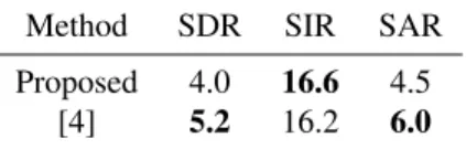
The second evaluation is dedicated to the user-guided source separation, where the proposed system was compared to [4] in a task of main melody (vocal source) extraction. The database consists on five 15s excerpts from the QUAERO source separation corpus. For each file and each system, the main melody pitch line has been localized, selected by means of the selection tool provided in both GUIs and finally ex-tracted. The quality of the estimated melody source is then quantified through the BSSEval toolbox [11], which gives the following measures: the Signal to Distortion Ratio (SDR), the Signal to Interference Ratio (SIR) and the Signal to Arte-fact Ratio (SAR). According to the results reported in Tab. 2, it seems that our system is slightly less efficient in a task of melody extraction. However, it can be noticed that it is more generic since it allows separating any polyphonic source whereas in [4], only monophonic sources can be extracted.

2_{The QUAERO (http://www.quaero.org) database will be soon available}

at http://www.tsi.telecom-paristech.fr/aao/en/software-and-database/

Method SDR SIR SAR Proposed 4.0 16.6 4.5

[4] 5.2 16.2 6.0

Table 2. Average SDR, SIR and SAR of the melody estimates using two systems.

7. CONCLUSION

In this study, we propose a new algorithm which accurately decomposes the CQT of an audio signal into a meaningful mid-level representation. Each time frame of the CQT is decomposed as a sum of harmonic notes, each note being modeled by means of fixed narrow-band harmonic templates. The presence of colored noise is also considered, and a new sparseness prior has been introduced for note activations. The BHAD algorithm has been evaluated in a task of multiple pitch estimation, and outperformed another state-of-the art algorithm. Finally, it has been proven that the BHAD model could be used for source separation, by offering a GUI where the user can select the notes he wants to extract. In future work, the authors plan to include a noise model for the notes, since for now, only noiseless harmonic instruments can be correctly being separated. Another outlook would be to automatically cluster the notes according to their timbre in order to isolate instruments in an unsupervised way.

A. EM UPDATE RULES WITH SPARSE PRIOR During the "maximization step" of the EM algorithm, one wants to maximize the joint log-probabilityQΛof all variables

(Λ denotes the set of all parameters). Using the same notation as in section 4, it can be proven that

QΛ= QΛ′+

︁

i,t

witln (θit) (20)

whereQΛ′depends on all parameters other thanθit= Ph(i, t).

With the addition of the sparseness prior, the maximization step is now replaced by a maximization a posteriori step. It does not change anything for the other parameters, but the new update rule forθitis obtained by maximizingQΛ+ ln (P r(θ)) with

respect to θ. It amounts to maximizing onΩ = ]0, 1]I×]0, 1]T the following functional under the constraintϕ(θ) = 1 − ︀ i,tθit= 0: � : Ω −→R θ_↦−→︁ i,t witln(θit) − 2β √ IT︁ i,t ︀θit. (21)

We know that the maximum exists onΩ since S is continuous and upper bounded by0 and its argument ˆθ verifies the first

order necessary conditions, proper to local maxima (Lagrange theorem): since� and ϕ are both differentiable, there exists a uniqueρ ∈ R such that:

∇Lρ( ˆθ) = 0 (22)

whereLρis the Lagrangian defined as:

Lρ : Ω −→ R

θ _{↦−→ �(θ) + ρ ϕ(θ).} (23) Equation (22) leads to:

∀(i, t), w_ˆit θit −β √ IT ︀ ˆ_θit − ρ = 0. (24) By studying the three casesmaxi,t

︁ −β4w2ITit

︁

< ρ < 0, ρ = 0 andρ > 0, it appears that︀

i,t w2 it β2IT > 1 if and only if ρ > 0. In that event, ∀(i, t), ˆθit= 2w 2 it IT β2_{+ 2ρw} it+ β √ IT︀β2_{IT + 4ρw} it , (25) ρ being the unique value for which︀

i,tθˆit= 1. This finally

proves eq.(15).

8. REFERENCES

[1] I. Virtanen, “Monaural sound source separation by nonnegative matrix factorization with temporal continuity,” IEEE Transactions on Audio Speech and Language Processing, vol. 15, no. 3, pp. 1066–1074, March 2007.

[2] S. Ewert and M. Müller, “Score informed source separation,” in Multi-modal Music Processing, Masataka Goto Meinard Müller and Markus Schedl, Eds., Dagstuhl Follow-Ups. Schloss Dagstuhl–Leibniz-Zentrum fuer Informatik, Dagstuhl, Germany, 2012.

[3] A. Ozerov, E. Vincent, and F. Bimbot, “A general flexible framework for the handling of prior information in audio source separation,” IEEE Transactions on Audio, Speech and Language Processing, vol. 20, no. 4, May 2012.

[4] J.-L. Durrieu and Thiran J.-P., “Musical audio source separation based on user-selected f0 track,” in Proc. of LVA/ICA, Tel-Aviv, Israel, March 2012.

[5] B. Fuentes, A. Liutkus, R. Badeau, and G. Richard, “Probabilistic model for main melody extraction using constant-Q transform,” in Proc. of ICASSP, Kyoto, Japan, March 2012.

[6] G.J. Mysore and P. Smaragdis, “Relative pitch estimation of multiple instruments,” in Proc. of ICASSP, Taipei, Taiwan, April 2009, pp. 313–316.

[7] B. Fuentes, R. Badeau, and G. Richard, “Adaptive harmonic time-frequency decomposition of audio using shift-invariant PLCA,” in Proc. of ICASSP, Prague, Czech Republic, May 2011, pp. 401–404. [8] “Companion website,” http://www.tsi.telecom-paristech.fr/aao/?p=756. [9] E. Vincent, N. Bertin, and R. Badeau, “Adaptive harmonic spectral decomposition for multiple pitch estimation,” IEEE Transactions on Audio Speech and Language Processing, 2010.

[10] S. Dixon, “On the computer recognition of solo piano music,” in Proc. of Australasian Computer Music Conference, July 2000, pp. 31–37. [11] E. Vincent, C. Févotte, and R. Gribonval, “Performance measurement in

blind audio source separation,” Audio, Speech and Language Processing, IEEE Trans. on, vol. 14, no. 4, pp. 1462–1469, 2006.