HAL Id: hal-01712155
https://hal.archives-ouvertes.fr/hal-01712155
Submitted on 8 Nov 2018HAL is a multi-disciplinary open access
archive for the deposit and dissemination of sci-entific research documents, whether they are pub-lished or not. The documents may come from teaching and research institutions in France or abroad, or from public or private research centers.
L’archive ouverte pluridisciplinaire HAL, est destinée au dépôt et à la diffusion de documents scientifiques de niveau recherche, publiés ou non, émanant des établissements d’enseignement et de recherche français ou étrangers, des laboratoires publics ou privés.
On various modeling approaches to radiative heat
transfer in pool fires
Kirk A. Jensen, Jean-Francois Ripoll, Alan A. Wray, David Joseph, Mouna
El-Hafi
To cite this version:
Kirk A. Jensen, Jean-Francois Ripoll, Alan A. Wray, David Joseph, Mouna El-Hafi. On various modeling approaches to radiative heat transfer in pool fires. Combustion and Flame, Elsevier, 2007, 148 (4), pp.263-279. �10.1016/j.combustflame.2006.09.008�. �hal-01712155�
On various modeling approaches to radiative heat transfer
in pool fires
Kirk A. Jensen
a,∗,1, Jean-François Ripoll
b,2, Alan A. Wray
c, David Joseph
d,
Mouna El Hafi
daFire Science and Technology Department, Sandia National Laboratories, Albuquerque, NM 87185, USA bCenter for Turbulence Research, Stanford University, Stanford, CA 94305, USA
cPhysics Simulation and Modeling Office, NASA Ames Research Center, Moffett Field, CA 94035, USA dEcole des Mines d’Albi, Laboratoire de Génie des Procédés des Solides Divisés, 81 013 Albi CT Cedex 09, France
Abstract
Six computational methods for solution of the radiative transfer equation in an absorbing–emitting, nonscatter-ing gray medium were compared for a 2-m JP-8 pool fire. The emission temperature and absorption coefficient fields were taken from a synthetic fire due to the lack of a complete set of experimental data for computing radi-ation for large and fully turbulent fires. These quantities were generated by a code that has been shown to agree well with the limited quantity of relevant data in the literature. Reference solutions to the governing equation were determined using the Monte Carlo method and a ray-tracing scheme with high angular resolution. Solutions using
the discrete transfer method (DTM), the discrete ordinates method (DOM) with both S4and LC11quadratures, and
a moment model using the M1closure were compared to the reference solutions in both isotropic and anisotropic
regions of the computational domain. Inside the fire, where radiation is isotropic, all methods gave comparable results with good accuracy. Predictions of DTM agreed well with the reference solutions, which is expected for a
technique based on ray tracing. DOM LC11was shown to be more accurate than the commonly used S4quadrature
scheme, especially in anisotropic regions of the fire domain. On the other hand, DOM S4gives an accurate source
term and, in isotropic regions, correct fluxes. The M1results agreed well with other solution techniques and were
comparable to DOM S4. This represents the first study where the M1method was applied to a combustion problem
occurring in a complex three-dimensional geometry. Future applications of M1to fires and similar problems are
recommended, considering its similar accuracy and the fact that it has significantly lower computational cost than
DOM S4.
Keywords:Fire; Radiation; Discrete ordinates; Discrete transfer; Monte Carlo; Ray tracing; M1model
* Corresponding author.
E-mail address:[email protected](K.A. Jensen).
1 Currently at Pixia Corp., Sterling, VA 20164, USA. E-mail address:[email protected].
2 Current address: Space and Remote Sensing Sciences (ISR-2), Los Alamos National Laboratory, P.O. Box 1663, NM 87545, USA. E-mail address:[email protected].
1. Introduction
Accurate prediction of the heat transfer from a large hydrocarbon fire, which can occur from an in-dustrial or transportation accident, is important for consideration of the thermal hazard to engineered sys-tems, personnel, and facilities. Fires of this scale typ-ically have relatively low velocities and high temper-atures and produce significant quantities of soot. The majority of heat transfer in such a fire is dominated by radiative emission from the high-temperature soot[1]. As a consequence, accurate solution of the radiative transfer equation is important for prediction of the resulting thermal hazard to an object exposed to the fire.
The cost and accuracy of a large fire simulation are strongly dependent on the choice of numerical model for solving the radiative transfer equation (RTE) gov-erning this phenomenon. The RTE is complicated by the fact that, in addition to the three-dimensional space variables and time commonly found in fluids problems, integration over all directions of propaga-tion is necessary at each point in the domain. The radiative source term, which couples to the energy equation, must be computed with sufficient accuracy to ensure a correct prediction of the evolution of the fire. Moreover, the scale of these fires, on the order of a few meters, as well as the existence of large spatial and temporal gradients in physical properties on microscales, would require simulations using mil-lions/billions of grid points and small time steps, mak-ing it impractical to routinely solve the governmak-ing equations directly.
Approximations, sometimes drastic, in terms of models or coarse meshes used for the radiative trans-fer are required, as is often done for turbulence, chem-istry, and soot production. For example, the work of
Porterie and Loraud [2,3] demonstrates the number
of assumptions and approximations needed for mod-eling the radiation in compartment fires. The most common method of accelerating the numerical solu-tion of the radiant transport is to limit the number of rays of integration. However, the choice of the minimum number of angles is often not rigorously justified, and the risk of choosing a poor resolution
exists in decreasing the computational time (see[4]
and references therein). The challenge, therefore, is choosing a computationally efficient numerical solu-tion method that predicts radiasolu-tion in fires, as well as radiative flux to objects inside and/or outside the fire, with sufficient accuracy.
For comprehensive coverage of the physics of fire and current research in fire modeling, the au-thors refer the reader to the following recent
re-views: Tieszen[5]and Drysdale[6]for fire dynamics;
Joulain[7]for pool fires; Novozhilov[8]concerning
modeling and computation of compartment fires; and, more recently, Sacadura[4]on radiation in fires.
In this study, six common numerical methods for solving the radiative transfer equation were compared when applied to a realistic synthetic full-field, three-dimensional fire (described below). The six methods include ray tracing, discrete transfer (DTM), discrete
ordinates (DOM), moment (with the M1 closure),
and Monte Carlo (MC). Ray tracing and the discrete transfer method are based on straightforward and di-rect integration of the integral equation by tracing a specified number of rays originating from each point throughout the domain. In contrast, the DOM con-sists of solving transport equations by finite volume methods along discrete directions. The angular inte-gration in DOM is performed with a select numeri-cal quadrature scheme. In this study, two quadrature schemes were investigated, including the traditional
S4 scheme with 24 angles, and the recently
investi-gated LC11formulation of Lathrop and Carlson with
96 angles[9]. The Monte Carlo method used here is
formulated in terms of net exchange and presumes the form of the probability density function for
effi-cient computations. The M1 moment method in this
study consists of a set of four hyperbolic equations obtained by integration of the RTE over frequency and angles. This method, however, requires a clo-sure model for the radiative presclo-sure. The maximum
entropy closure [10] is used here. Our study is
un-fortunately limited to the only methods which were available to us.
General descriptions of these methods can be
found in [11–14], and more details will be covered
below with comprehensive references describing the implementations. The discrete transfer and discrete ordinates methods are commonly used to solve radi-ation in fires. For example, the DTM is utilized in
Vulcan[15,16], JASMINE[17], and SOFIE[18], and
DOM is used in various French fire codes[2,3,19]and
SIERRA/Syrinx [20,21]. The Monte Carlo method
has been used for computation of radiation in com-partment fires[22], although it is not generally used
in fire codes, given its computational cost. The M1
method has not been applied previously to a three-dimensional fire problem to the authors’ knowledge.
To compare the accuracy of the commonly used
DTM and DOM techniques, as well as the M1
method, the solution of the heat flux and radiative source terms are required. Unfortunately, a data set of these quantities is unavailable for this purpose, as ex-plained in the next section. Therefore, the ray tracing and Monte Carlo techniques were used to obtain these reference-solution fields. With the “known” radiative fields obtained from Monte Carlo and ray tracing, the
accuracy of the DT, DO, and M1 methods can be
res-olutions and general accuracy of the computational scheme were addressed in this study.
This represents the first study in which the M1
moment formulation is applied to the computation of fires. The closure approximation was first introduced
by Minerbo [10]while searching for an appropriate
Eddington factor to close the radiative pressure term, and has been developed over the past 20 years by the
efforts of[23–25]and numerous works cited in[26].
However, it has received little attention in the com-bustion community and little theoretical description
of M1 exists in modern radiation textbooks [11,12].
Consequently, the implementation details for applica-tion to fires will be discussed below. This method is particularly attractive because it has the lowest the-oretical computational cost compared to the other
methods. The angular dependence in M1 is handled
analytically, thus removing two variables from the in-tegration of the gray RTE (leaving time and position as the remaining variables).
The paper is constructed as follows. The moti-vation for and creation of the synthetic fire are de-scribed, including the geometry of the facility it rep-resents, the computation of the fire, and the boundary conditions used. This description is followed by the definition of the radiant transport problem and the presentation of the six computation methods used to solve the radiation in this fire field. Discussion of the numerical results focuses on two aspects of solving the radiative transport problem of interest to fire mod-eling. First, an angular study was performed and the effects of choosing too low an angular resolution on the coupling to the fire hydrodynamics are consid-ered with the ray tracing and discrete transfer meth-ods. Second, the six methods were used to solve the radiative transfer of the fire, and particular attention was given to both the radiative flux and the radia-tive source term profiles. The reference solutions from Monte Carlo and ray tracing were used to quantify and compare the accuracy of these variables obtained
by the discrete transfer, discrete ordinates, and M1
moment methods.
2. Synthetic fire
Solution of radiant transport in a hydrocarbon fire requires knowledge of the absorption coefficient and emission temperature fields throughout the participat-ing medium. Those coefficients involve knowledge of
the soot, CO2, and H2O concentrations and the
tem-perature. Ideally, the radiative properties would be fully spatially resolved so that no filtering of the radia-tive transport equation was required. Unfortunately, such a data set is nowhere near obtainable. For in-stance, experimental measurements as detailed as a
direct numerical simulation (DNS) of the turbulent
reacting flow field would require between 1012 and
1015 measurement points (corresponding to between
200 and 20 µm needed for measuring the soot volume fraction accurately within the gradient of temperature in a 2-m fire).
The goal of the current study is not to assess ra-diative transport methods for DNS solutions of large fires, for the same reason that data sets do not exist— they are not obtainable. Current and foreseeable com-putational strategies for large fires will require that the radiative transport equations (along with the turbu-lent reacting flow equations) be modeled. The filtered radiative transport equation then contains effective emission temperature and absorption properties that account for the high spatial frequencies that are not resolvable on the grid. These models are sometimes referred to as turbulence–radiation interaction mod-els (TRI). Typically, correlations of the form Ys˜T5,
where Ys is the soot volume fraction and T the
tem-perature, are needed as soon as “low resolution” pro-files are used. (The reader should note here that using a fourth power of ˜T in the emission term is not appro-priate for large fires because it neglects TRI and leads to large error.) Hence fire temperatures, for which there are many data sets, cannot be used as a valida-tion field.
Unfortunately, data sets for even filtered proper-ties are not available either, except for limited
mea-surements along the centerline and a radial [27],
not enough for assessing three-dimensional radiation transport methods. The lack of measurements is due
to complex fire dynamics[28]and difficulties
associ-ated with diagnostic instruments in high-temperatures
sooting environments [1,29,30]. Given this lack of
comprehensive experimental data, a synthetic 2-m JP-8 fire was created with the Vulcan fire simulation tool
from Sandia Albuquerque[15]. Vulcan has been used
in recent years to simulate pool fires resembling those in the Fire Laboratory for Accreditation of Models and Experiments (FLAME) facility in Albuquerque,
New Mexico[16].
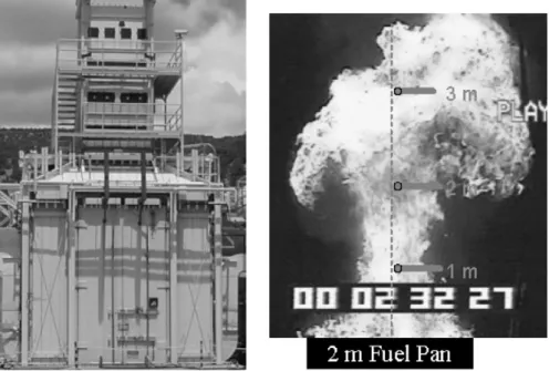
FLAME consists of a 6.1-m square water-cooled wall structure with a 6-m air ring on the floor and a 2-m fuel pan elevated approximately 1.6 m above
ground.Fig. 1shows (left) the exterior of the FLAME
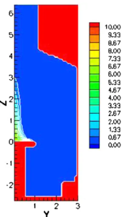
facility and (right) a video still image during a 2-m JP-8 fire. The heights above the fuel pan are indicated by the horizontal bars in the figure, and the scale of the fuel pan is included at the bottom. The 3D computa-tional mesh of this facility consists of a 92× 92 × 120 Cartesian grid and its central plane contour plot is
shown in Fig. 2 (left). The dark cells in this figure
represent the walls, the air inlet ring (bottom), the fuel pan (center), and the atmosphere outside the chimney (top outer edges). It has been confirmed
experimen-Fig. 1. (Left) The FLAME facility for fire experiments and (right) a still image from video taken during a puff of a 2-m JP-8 pool fire test.
Fig. 2. (Left) A two-dimensional contour view of the computational domain modeling the FLAME facility and (right) the emission temperature (( ˜T4)1/4) contours along the centerline planes of the three-dimensional synthetic fire.
tally[31] that the four corners of the square facility do not influence the axial symmetry of the source air flow, and the resulting fires are indeed axially sym-metric. The calculations were performed using the full 3D data set as input. The symmetry of all so-lutions was verified and, therefore, results are only presented for various axial and radial locations along the central plane of the facility.
To compute the fire, the fluid conservation equa-tions are solved using a Reynolds-averaged Navier–
Stokes (RANS) approach, with sufficient iterations from ignition to reach a steady-state solution. The emission temperature, defined as ( ˜T4)1/4, is plotted inFig. 1(right) and accounts for TRI. To obtain a rel-evant estimate of the emission temperature, a simple model for turbulent radiation interactions is used em-ploying a double delta function representing soot in the flame sheets and soot that has been mixed into the
Fig. 3. A two-dimensional contour view of the absorption coefficient κ.
are related to an estimate of the volume fraction of flame in each cell.
Vulcan treats the fire as a gray absorbing–emitting
medium with negligible scattering[32]. The
absorp-tion coefficients contain contribuabsorp-tions mostly from soot particles but also include contributions from carbon dioxide and water vapor absorption at se-lect wavelengths with an empirically based wideband model. The model for these coefficients assumes that the medium is gray since soot is the dominant
ab-sorbing and emitting species[33]as we now explain.
Soot is a broadband emitter the spectral absorption of which follows a linear spectral law on the whole
fre-quency spectrum (see for instance[34]). This law is
evaluated here with the coefficients of[35]and is in-tegrated over the whole frequency spectrum in order to obtain a Planck mean coefficient which is used af-terward in the RTE. Thus, the nongray character of soot is accounted for through this Planck mean coef-ficient. The filtered absorption coefficient is plotted in Fig. 3.
Normally in the solution of the RTE, it is nec-essary to know the optical properties of all surfaces with which radiative energy can come in contact. At a surface, all incident energy must be absorbed,
trans-mitted, or reflected—that is, α+ τ + ρ = 1, where
α, τ , and ρ are the surface absorptance, transmit-tance, and reflectransmit-tance, respectively. When the domain of computation is as complex as the FLAME
facil-ity (seeFig. 2), implementing the prescribed
bound-ary conditions uniformly across five different codes proves challenging. Instead, an alternative approach using “ghost cells,” which can be considered similar to the immersed boundary conditions technique, was
used to overcome this difficulty. The domain is con-sidered as an open domain throughout which radiation can travel. The walls and the pan are simulated by cells having a constant and very large opacity (a few
hundred m−1) and an ambient temperature (293 K),
such that the walls and the pan are artificially main-tained in a black and cold state, conditions that hold in the FLAME facility. At the exhaust opening at the top of the chimney, it is assumed that all energy leaves
unimpeded (τ= 1).
3. Solution methods of radiative transfer
The gray radiative transfer equation (RTE) de-scribes the change in radiation intensity, I , through an absorbing and emitting gray medium along a path of length ds in a solid angle Ω defined around the di-rection of propagation s[11],
(1) dI (s)
ds =κIb− κI (s),
where Ib = σ ˜T4/π is the blackbody intensity at
temperature T , σ is the Stefan–Boltzmann constant, and κ is the filtered absorption coefficient (based on a Planck mean coefficient). The gray intensity I represents here a spectral intensity I (ν) which has
been integrated on the whole frequency spectrum ν∈
[0, +∞[. Ibaccounts for the temporal fluctuations of
the fourth power of the temperature due to TRI, and thus I does too.
For most heat transfer applications, the primary engineering quantities of interest are the net incident radiation (G), the radiative flux (qr), and the
diver-gence of the radiative heat flux (∇ · qr), called the
radiative source term hereafter. These quantities can be derived from the following integrals of intensity over solid angle:
G= ! 4π I (s) dΩ, qr= ! 4π I (s)s dΩ, and (2) ∇ · qr= κ(4πIb− G).
Solution of the RTE (Eq.(1)) and Eqs.(2)using each
solution scheme is outlined separately below.
3.1. Discrete transfer method (DTM)
The discrete transfer method (DTM) used in Vul-can is an enhanced version of the original model
pro-posed by Shah [36,37]. The enhancements were
se-lected to obtain an acceptable compromise between accuracy and calculation speed. The technique will be tested by comparing the results obtained herein with those obtained from verified and highly accurate Monte Carlo and ray-tracing techniques.
Within the computational domain a radiation box is defined to speed the calculation by focusing on the region with high thermal emission. This box de-fines where rays originate in the tracing technique. For this study, the box was defined as the smallest grid-conformal parallelepiped encompassing all con-trol volumes with a emission temperature greater than 800 K.
For each node on the boundary of the box, a speci-fied number of rays are emitted over a hemisphere and followed to the boundary of the calculation domain; a corresponding ray is followed back from the bound-ary to the original point, and on to the next boundbound-ary. Along these traces, the change of intensity from ab-sorption and emission is calculated over each control volume in the path with proper weighting given to the solid angle and the originating projected area.
The change of intensity for the ray within a control volume is found from a recurrence relation obtained from analytical integration of Eq.(1),
(3) In+1= Inexp(−κδs) + Ib"1− exp(−κδs)#,
where δs is the distance over which the beam passes through the control volume.
The source term for the energy equations, Eqs.(2), is found by summing the net gain or loss of radiation energy in each control volume intersected during a ray trace. The contribution to the source term from one beam i passing through a control volume n is given by
(4) Sn,i= (In+1− In)sidA dΩ,
where dA is the area from the element at the ray origin
boundary and Ωiis the solid angle represented by the
beam. The total radiant source term for the nth control volume is found by summing over N total beams:
(5)
QrdV = $
i=1,N
Sn,i.
The heat flux to a surface is not explicitly cal-culated throughout the field of Vulcan, but rather at selected surfaces (i.e., cell faces). The hemispherical
flux in W/m2is derived from this model by
integrat-ing all incomintegrat-ing rays on a surface. This integration requires a large number of rays to be traced from each node of the radiation box to be accurate, but from ex-perience it has been found to be quite fast when a limited number of selected surfaces are used. To com-pare to the other methods, the hemispherical fluxes to the common surface shared by two adjacent cells were summed for the equivalent of a 4π integration.
3.2. Discrete ordinates method (DOM)
The discrete ordinates method was first introduced
by Chandrasekhar [38] and has been widely used
since then in radiative transfer applications. A ma-jor advantage of this method is that it can be sim-ply coupled with the hydrodynamics system using the
same structured or unstructured grid[39]. The DOM
is based on the discretization of the RTE (see Eq.(1))
over a chosen number, Ndir, of discrete directions,
si(µi, ηi, ξi), contained in the solid angle 4π and
as-sociated with weights wi. Koch and Becker[9]
com-pared several types of angular quadrature schemes, of which the two that were selected for this study are S4
and LC11. The S4quadrature scheme, with 24
direc-tions, is often chosen for its computational efficiency.
The LC11scheme, with 96 directions, was chosen for
its higher accuracy. The ordinate directions for each of these quadrature schemes are tabulated inTable 1.
The RTE is solved for every discrete direction si
using a finite volume approach. The integration of the RTE over the volume V of an element limited by a surface Σ with outer unit normal n, and application of the divergence theorem yields
(6) ! Σ Is · n dΣ = ! V " κIb− κI (s)#dV .
The domain is discretized in control volumes which, in this study, are regular hexahedra, but can also be
a nonregular mesh for this formulation. Taking Ij to
be the average intensity over the j th face, associated with the center of that face, and taking Ib,P and IP to be the average intensities over the volume V , as-sociated with the center of the cell, P , Eq.(6)can be discretized as
(7)
N$face
j=1
Ij(si· nj)Aj= κV (Ib,P− IP),
where the scalar product of the ith discrete direc-tion vector with the normal vector of the j th face of the considered cell is defined by si · nj = µinxj +
ηinyj+ ξinzj. Ibis assumed to be constant and equal
to Ib,P over the volume V , and Ij is taken constant
over each face. For each cell, the incident radiation G given in Eqs.(2)is evaluated at the center by
(8) G≃ Ndir $ i=1 wiIP(si).
For a gray medium, the divergence of the radiative heat flux is obtained from Eqs.(2). To solve Eq.(7), a spatial differencing scheme based on the mean flux
(DMFS), proposed by Ströhle et al.[40], was used.
This scheme uses the decomposition
(9) IP=1
2Iout+ 1 2Iin,
where Iin is the weighted average of the intensities
Table 1
Ordinate direction components of S4and LC11
Quadrature µ η ξ w S4 0.2958759 0.2958759 0.9082483 0.5235987 0.2958759 0.9082483 0.2958759 0.5235987 0.9082483 0.2958759 0.2958759 0.5235987 LC11 0.1891433080 0.1891433080 0.9635609052 4π/96 0.1891433080 0.9635609052 0.1891433080 4π/96 0.9635609052 0.1891433080 0.1891433080 4π/96 0.4486223380 0.4486223380 0.7729657144 4π/96 0.4486223380 0.7729657144 0.4486223380 4π/96 0.7729657144 0.4486223380 0.4486223380 4π/96 0.6865960430 0.6865960430 0.2391061427 4π/96 0.6865960430 0.2391061427 0.6865960430 4π/96 0.2391061427 0.6865960430 0.6865960430 4π/96 0.8795381380 0.4758283974 0. 2π/96 0.4758283974 0.8795381380 0. 2π/96 0.8795381380 0. 0.4758283974 2π/96 0.4758283974 0. 0.8795381380 2π/96 0. 0.8795381380 0.4758283974 2π/96 0. 0.4758283974 0.8795381380 2π/96
average of the intensities leaving the cell. Substituting Iout from Eq.(9)into Eq.(7), and after some algebra
(see[41]for details), the following expression for IP
results, IP=% 1 2κV Ib− $ j,Dij<0 DijAjIj & (10) '% 1 2κV + $ j,Dij>0 DijAj & ,
where Dij = si · nj. After IP is calculated from
Eq. (10), the radiation intensities at those cell faces at which Dij >0 are set equal to Iout, obtained from
Eq.(9). In solving the RTE along a given discrete di-rection, the control volumes should be treated follow-ing a sweepfollow-ing order, dependfollow-ing on the considered direction and defined such that the radiation intensi-ties are known at the upstream cell faces. A specific algorithm is then used to define the order of the com-putation of the cells.
A radiative heat transfer code called DOMASIUM has been developed based on this method to com-pute the radiative transfer in complex geometries,
mainly for combustion applications [41]. Radiation
is solved on hybrid grids (hexaedra and tetraedra),
imposed by the CFD code developed at CERFACS3
which solves the hydrodynamics by LES techniques. To take into account gas combustion spectral lines, an SNB-ck model has been implemented. In this
3 Centre Européen de Recherche et de Formation Avancée en Calcul Scientifique.
work, only regular cells and simple gray medium are considered; nevertheless, this comparison repre-sents a validation of the code in its simplest formula-tion.
3.3. Monte Carlo method—net exchange formulation (MCM-NEF)
Monte Carlo methods (MCM) have often been used to produce highly accurate solutions in the
process of validating other numerical methods [42,
43]. They first appeared in the literature as strict nu-merical implementations of stochastic photon
trans-port models[44,45]. The very large number of
real-izations required to achieve convergence shows the limitations of the classical Monte Carlo algorithms, particularly when optically thick media are encoun-tered[46,47]. To overcome these difficulties, a math-ematical formulation using the net exchange
formula-tion (NEF)[48,49], together with adapted probability
density functions, has been proposed to improve the
variance reduction procedures [50]. In addition, to
treat each ray, computer graphics techniques are ap-plied to reduce the computational time. A new space subdivision called voxels, defined below, enables the use of efficient algorithms for intersection calcula-tions[51].
Taking Pi as a point within the volume Vi and Pj
within Vj, we denote the position vectors of Pi and
Pj as rPi and rPj. The net radiative exchange
be-tween two volumes Vi and Vj, ϕ(Vi,Vj), or a volume Vi and a surface Sj, ϕ(Vi,Sj), or two surfaces Si and Sj, ϕ(Si,Sj), is expressed for black walls and
nonscat-tering media as (11) ϕ(Vi,Vj)= ! Vj ! Vi κ(rPi)κ(rPj)τ (sij) sij2 ×(Ib(rPi)− Ib(rPj))dVidVj, (12) ϕ(Vi,Sj)= ! Sj ! Vi |n(rPj)· s|κ(rPi)τ (sij) sij2 ×(Ib(rPi)− Ib(rPj))dVidSj, (13) ϕ(Si,Sj)= ! Sj ! Si |n(rPi)· s||n(rPj)· s|τ(sij) sij2 ×(Ib(rPi)− Ib(rPj))dSidSj, where sij = sj− si= |rPj− rPi|, and (14) s =(rPj − rPi) |rPj − rPi| ,
with n the normal vector to the surface S, κ the gray absorption coefficient, and τ (sij)the spectral
trans-missivity along a straight line between Pi and Pj
given by (15) τ (sij)= exp * − sj ! si κ(s)ds + .
The radiative source term for a volume Vi and the net
heat flux at a surface Si are computed by taking into
account their radiative exchanges with all the other volumes and surfaces,
(16) Sr(rPi)= ! Vi ∇ · qrdVi= Ns $ j=1 ϕ(Vi,Sj)+ Nv $ j=1 ϕ(Vi,Vj) and (17) qw,net,i= Ns $ j=1 ϕ(Si,Sj)+ Nv $ j=1 ϕ(Si,Vj),
where Nsis the number of surfaces and Nvthe
num-ber of volumes.
One way of evaluating the multiple integrals in the expressions for the net exchange rates, Eqs.(11), (12), and (13), is to use a Monte Carlo method, which is described next.
Considering that each radiative exchange can be represented as an integral I of a function f over a domain D, (18) I = ! D f (x)dx.
An arbitrary probability density function (PDF), p, defined and strictly positive on the integration
do-main D is introduced. The weight function W (x)=
f (x)/p(x)is used to write I = ! D f (x) p(x)p(x)dx= ! D W (x)p(x)dx.
Given a random variable X, distributed according to p, and a function of that variable, g(X), we let I rep-resent the expectation of g(X). Estimating I with N samples g(xi), where xi is the ith realization of the
random variable X gives
I = E(g(X))≈ 1 N N $ i=1 g(xi)=,g(X)-N, (19) where I = lim N→∞ , g(X)-N.
Then the standard deviation of the estimate is calcu-lated as σ (⟨g(X)⟩N)=√1Nσ (g(X)), where σ (g(X))
is the standard deviation of g(X). It is approximated by (20) σ",g(X)-N#≈ √1 N .(, g(X)2-N−,g(X)-2N). In this last expression the variance depends on the function g, which itself depends on the PDF. To per-form efficient Monte Carlo simulations, the choice of the PDF is crucial. More details can be found in [50,52].
It should be noted that the results presented in this paper have a standard deviation of about 1% or less. Moreover, this Monte Carlo algorithm has another feature that combines the PDF optimization with computer graphics techniques in order to opti-mize the ray-tracing procedure. It applies an efficient algorithm to evaluate the intersections between paths and surfaces and uses voxels. Voxels, or “volume el-ements,” are cells defined in terms of homogeneous emission temperatures and molar fraction levels that subdivide the space, but differently from the CFD grid
[51]. To save computational time, a good compromise
between the time to treat each voxel and the level of grid subdivision has to be determined.
3.4. Ray tracing
This method treats the RTE as a set of first-order ordinary differential equations (ODEs), with one ODE for each spatial point, directional angle, and frequency. In the gray problem considered here, the frequency dependence is handled by analytically inte-grating the RTE over frequency. At each spatial point
x, a set of rays is considered to project inward toward
angle space in such a way as to allow accurate inte-gration over that space to compute the net incident radiation and the heat flux. For the fire problem, the rays are followed outward from the chosen point un-til they intercept a wall or the exit of the chimney. At such a boundary point the initial value of the incom-ing radiative intensity is set to equilibrium (I = Ib).
From this initial value the RTE is integrated forward along the ray to the chosen spatial point, and the value at that point is saved for inclusion in angular integrals involving I (x, Ω).
The method of integration along a ray assumes that, within each step of the quadrature, the source Ib and opacity κ are constants equal to their interpolated values at the center of the step. With this assumption, I (s, Ω) can be advanced from one end of the step, s0, to the other, s1, according to the following rule:
I (s1,Ω)= I (s0,Ω) exp"−κ|s1− s0|#
(21) + Ib"1− exp"−κ|s1− s0|##.
Once the full set of angular values I (x, Ω) is ob-tained at the point x, angular integrals, such as those in Eqs.(2), are performed to compute quantities of in-terest.
3.5. Moment methods and the M1closure
A system of equations for two moments, the net incident radiation G and the radiative flux qr, can be
extracted from the gray RTE, Eq. (1), by integrating
over all directions. The system is given by
(22) 1 c∂tG+ ∇ · qr= κ " 4σ ˜T4− G#, (23) 1 c∂tqr+ ∇ · (DrG)= −κqr,
using the same notation for the other solution
meth-ods above. The M1 closure [23,24] is given by the
Eddington tensor Dr obtained by the maximum
en-tropy closure [10,25]. More references concerning
this model can be found in[26]. The Eddington
ten-sor is computed from the Eddington factor χ and the anisotropic factor f= qr/Gas
(24)
Dr= 1− χ2 Id +3χ2− 1f ⊗ f
f2 ,
where Id denotes the identity matrix, f the Euclidean
norm of f, and ⊗ stands for the dyadic product. The
Eddington factor χ is given by
(25)
χ (f )= 3+ 4f
2
5+ 2/4− 3f2.
The Eddington tensor Dr, which plays the role of a
flux limiter, comes from an underlying radiative in-tensity that is able to describe both a beam by a Dirac
function and isotropic radiation by a Planck function.
Hence, the M1 model is able to predict radiation in
opaque, semiopaque, or transparent media and, as we show below, is particularly suited for the computation of radiation in fires. The numerical scheme used to solve this model is given in[53].
4. Results and discussion
In the following computations, the Monte Carlo
code provides the radiative source term (Eqs. (2))
of reference. The ray-tracing code obtains the same values for this term when angular convergence is en-sured. Angular convergence of this code is reached for 20,000 angles. This has been checked with compar-ing with a 80,000 angles computation. The ray-traccompar-ing code with 20,000 angles is thus also considered as a second reference code and provides the reference ra-diative fluxes, which our MC code does not provide (only by a lack of implementation).
4.1. Angular resolution and coupling
In this section, the number of angles needed for the baseline fire computation is investigated using the ray-tracing code. This result should aid future choice of angular resolutions, quadrature schemes, and
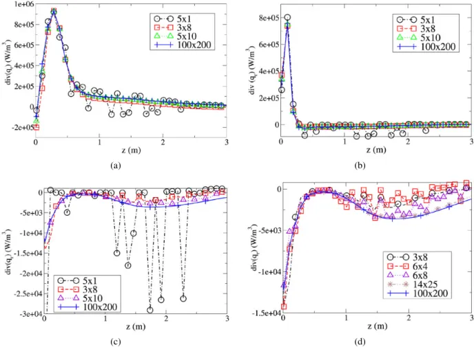
solu-tion methods.Fig. 4shows the radiative source term,
div(qr), plotted as a function of elevation above the
fuel pan for several radial positions with distinct ra-diant transport behavior. Inside the fire at a radius
of r = 0.43 m, high emission temperature radiation
is incident from all directions, creating an isotropic environment. At larger radii within the fire (e.g., at
r = 0.7 m), conditions are such that the radiation
from high-temperature soot is near isotropic. At all positions at high elevations above the fuel pan and at radial positions outside the fire (i.e., r > 1.0 m for this fire), the field is anisotropic since high emission temperatures exist only on one side of the point of in-terest. The reference solution is shown with 20,000
angles (µ= 100 × φ = 200), which was sufficient for
angular convergence.4 It is apparent that for low
an-gular resolutions, less than approximately 50 angles, predictions of the source term are poor both inside (Figs. 4a and 4b) and outside (Figs. 4c and 4d) the fire. When only 5 or 10 angles were used, which is likely during the initial stages of a simulation to ac-celerate it toward a steady solution, it was found that ray effects were dominant, meaning that a hot source may or may not transport heat to each distant point
4 All ray-tracing results presented were calculated with this resolution.
(a) (b)
(c) (d)
Fig. 4. Radiative source term, div(qr), in (W/m3) as a function of elevation above the fuel pan computed by ray tracing with the specified angular resolution µ× φ at radial positions (a) r = 0.43 m, (b) r = 0.70 m, and (c, d) r = 1.03 m.
according to the angles chosen. Results vary greatly based on the choice of angles for integration.
Inside the fire (Figs. 4a and 4b), in the isotropic regions, it is found that at least 50 rays are needed to get results close to the reference profile. Outside the fire (Figs. 4c and 4d), it is shown that the use of 350 angles gives good agreement and ray effects are reduced or eliminated. Hence, because such resolu-tions are needed for accuracy, a high computational cost is expected. Nevertheless, these results must be balanced by the fact that neither special quadratures, nor particular choices of angles have been used herein to try to improve the accuracy of the results for low angular resolution. This feature will be illustrated in the next sections. In the ray-tracing solver,
an-gles are uniformly distributed in µ= cos(θ) and φ,
which may not be the optimal choice. Undoubtedly, a better choice of angles and/or quadratures could de-crease the number of angles needed to get accurate results.
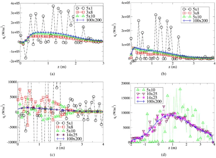
Fig. 5 shows profiles of the radial component of the radiative flux as a function of elevation at radial lo-cations inside (Figs. 5a and 5b) and outside (Figs. 5c and 5d) the fire. Similarly to the source terms, it is apparent that angular resolutions of less than 50 rays lead to poor prediction of the flux both inside and
outside the fire. Moreover, in the higher anisotropic regions outside the fire, more than 250, ideally 350, rays are required to reasonably match the reference solution.
The importance of the ray effects are emphasized
by considering a coupled fire problem.Fig. 6shows
the predicted hemispherical heat flux incident on a
surface at a fixed location in the fire at radius r =
0.55 m and height z= 0.5 m above the fuel pan as
a function of time in the 2-m fire. The source term predicted at each angular resolution was coupled to the hydrodynamics and evolved in time from igni-tion. Radiation was solved by the DT method for various angular resolutions from as low as 24 rays to as much as 350 rays (as suggested by the results inFigs. 4 and 5). Of these results, it is seen that 24 angles does not lead to an accurate solution of the ra-diative flux and contains strong temporal fluctuations. Since the coupling between radiation and hydrody-namics is strong in fires, a poor computation of the radiation can, for instance, lead to extinction or to an over/under-estimation of soot formation. Since these phenomena are highly nonlinear and strongly cou-pled, chained effects on the resulting fires can occur as in the two following scenarios. The prediction of excess soot (which corresponds to high opacity) can
(a) (b)
(c) (d)
Fig. 5. Radial component of the radiative flux (W/m2) as a function of elevation above the fuel pan computed by ray tracing with the specified angular resolution µ× φ at radial positions (a) r = 0.43 m, (b) r = 0.70 m, (c) r = 1.03 m, and (d) r = 2.55 m.
Fig. 6. Temporal evolution of the radial component of the hemispherical heat flux to a surface at an elevation z= 0.5 m and radial position r= 0.55 m with a radially outward normal calculated by the discrete transfer method with various angular resolutions.
lead to excessive heat loss by radiation, which then leads to a smaller, weaker fire, or even to extinction. On the other hand, an underestimation of soot can lead to low radiation heat losses, implying a hotter, larger fire. Thus, low angular resolution for radia-tion should be avoided for fire computaradia-tions to ensure
proper coupling and corresponding fire behavior par-ticularly during transients.
It is also seen fromFig. 6that using 80 rays seems to be a good compromise between speed and accuracy for the Vulcan results to be close to convergence, but the fluctuations are still notable. It is reasonable, then,
as a result of these observations, to run a fire simula-tion with Vulcan with 80 angles to allow the fire to develop more rapidly, and later use 350 angles for a converged solution with less fluctuations. For the re-mainder of this study, all Vulcan results are reported for the higher, converged solution at a resolution of 350 angles obtained after the initial progression with 80 angles to a steady-like state.
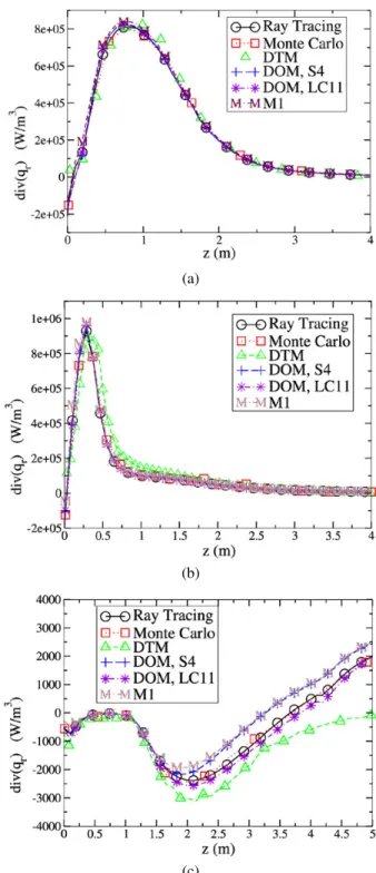
4.2. Radiative source term
A comparison of the radiative source term
(div(qr)) calculated by each method is shown in
Fig. 7. Since this quantity couples the hydrodynam-ics system to the radiant transport solution, accurate computation is mandatory for obtaining the correct fire profile. A positive value of the source term repre-sents a net emission, and vice versa, negative values imply that net absorption is occurring at that point. The ray-tracing code with high angular resolution and the Monte Carlo code were used to determine reference solutions of this quantity. Both of these codes found similar solutions, within the 1% accu-racy of the Monte Carlo technique, at all points in the
facility. Figs. 7a and 7b show the source term
pro-files for radial positions r= 0.29 m and r = 0.43 m
inside the fire as a function of elevation above the pan. Good global agreement with minimal discrepan-cies is found between all methods. The differences are sufficiently small that they would not have a strong effect on the coupled energy equation. The similarity in accuracy of these results can be ex-plained by the fact that the radiation inside the fire is mainly isotropic, f < 0.2, which would lessen ray effects.
For points just outside the fire at r= 1.15 m in
Fig. 7c, more discrepancies are seen among the meth-ods. The lower accuracy is likely due to the less isotropic nature of radiation in this region; however, it is noted that this far outside the fire the small er-rors would not affect the dynamics of the fire. The
DOM S4 method is less accurate than DOM LC11,
most likely because its lower angular resolution of 24 angles (versus 96 of LC11) results in ray effects.
The M1 model gives results nearly identical and as
accurate as DOM S4. These methods slightly
under-estimate absorption outside the fire, while the DTM overestimates it to a similar degree. Despite the dis-crepancies, the magnitude of the source term is suf-ficiently small in this region that less accuracy is ac-ceptable.
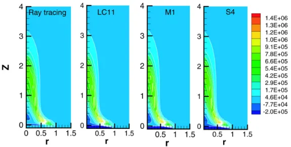
In Fig. 8, two-dimensional contour plots of the source term along the central plane of the fire are
(a)
(b)
(c)
Fig. 7. Radiative source term (W/m3) as a function of ele-vation above the fuel pan at radial positions (a) r= 0.29 m, (b) r= 0.43 m, and (c) r = 1.15 m.
shown for the ray tracing, DOM S4, DOM LC11, and
M1 methods.5 It should be noted that the high
ab-sorption values near the pan at z= 0 and r ! 1.0 m
are produced by the artificially high opacity of ghost cells modeling the fuel pan and are not considered
5 Monte Carlo and DTM results were not available for every node of the domain and are, therefore, not plotted here.
Fig. 8. Contour plots of the radiative source term (W/m3) along the central plane of the fire domain computed by, from left to right, ray tracing, DOM LC11, M1, and DOM S4. Radial and axial distances have units of meters.
in comparison of the solution methods.6 In this
fig-ure, no noticeable difference is apparent in the source term computation among the four methods considered here. In particular, the large positive values, indicat-ing emission and representindicat-ing the radiative coolindicat-ing,
are the same, as shown in detail inFigs. 7a and 7b.
This finding is encouraging for the low-cost M1and
S4 methods, as accurate determination of the source
term ensures a solution coupled to the hydrodynam-ics that will evolve properly. Negative values of the source term, indicative of absorption zones, are also visible inFig. 8 inside the fire and indicate the pre-heating cone of the fire. In this region, the chemistry evolves strongly and most of the radicals and pollu-tants are formed or preformed. Moreover this zone is heated by absorption of the radiation coming from the hot regions of the fire, which is here correctly com-puted by all methods. To conclude, it has been found that all six methods give similar predictions of the ra-diative source term.
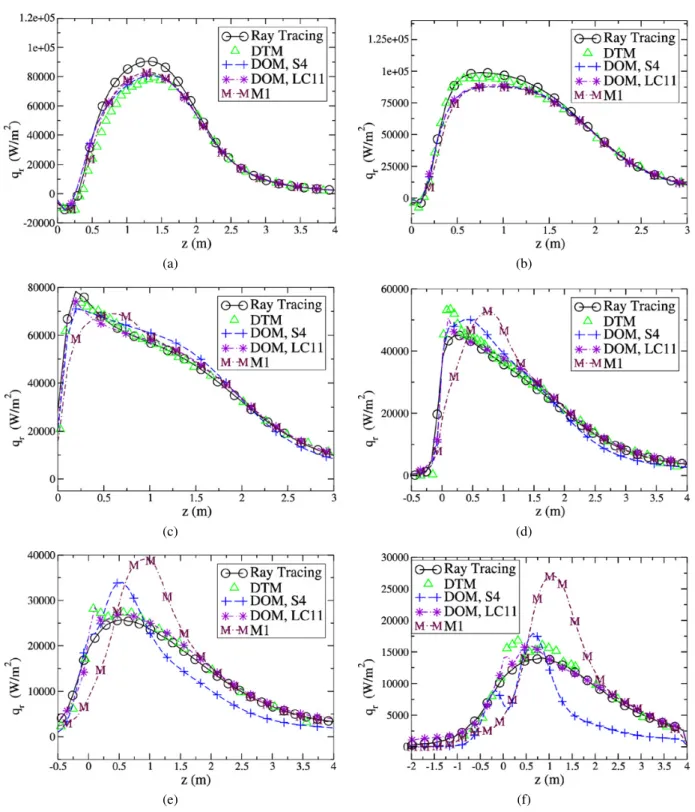
4.3. Radial component of the radiative flux
Fig. 9 shows the radial component of the
radia-tive flux in W/m2 as a function of elevation above
the fuel pan for radial locations inside and outside the fire. The ray-tracing code at a high angular resolution was used to generate the reference solution since the computation of the flux field by the Monte Carlo code
was not yet available. In Figs. 9a and 9b the fluxes
inside the fire are compared. All methods roughly agree and compute consistent trends. At higher ele-vations, for z > 1.5 m, all methods fully agree since
6 The very small differences between the emission and ab-sorption terms is amplified by the large opacity chosen for the wall (600 m−1).
strong emission temperature and opacity gradients are
absent. The three methods, M1, S4, and LC11, are
in good agreement with the reference solution, but
slightly underestimate the flux.Figs. 9c and 9dshow
the radial radiative flux profiles still inside the fire at a
radius of r= 0.7 m and at the edge of the fuel pan at
r= 1.03 m. The DTM method agrees globally with
the others but overestimates the fluxes close to the
fuel pan (z= 0) for r = 0.7 m. Similar to the source
term computation, the M1and S4methods give
com-parable results, which is very encouraging for M1in
which the angular dependence of the radiation field was treated with the analytical closure approximation.
No noticeable difference was observed between S4
and LC11, whose results agree well with those of the
ray-tracing method.
The fact that S4 computes both flux and source
terms relatively well, when linked with the angular
studies of Section4.1, implies that 24 angles should
be enough inside the fire provided that the S4 set of
angles is chosen. This result constitutes an improve-ment by a factor of two of the number of angles needed, compared to the use of uniformly distributed angles. (It should be also noted that the 24 angles of DTM used in the time evolution study in the previous section were not optimally chosen as are the 24 rays in the S4technique.)
Fluxes outside the fire are shown inFigs. 9e and
9f. The DTM method gives accurate results, in
agree-ment with the ray-tracing solver. The DOM LC11also
gives accurate results, which leads to the conclusion that around a hundred angles should be enough to compute radiation at 1 or 2 diameters away from the fire provided an accurate quadrature is chosen. This constitutes an improvement by a factor of 3 compared to a uniformly spaced angular set, which apparently
(a) (b)
(c) (d)
(e) (f)
Fig. 9. Radial component of the radiative flux (W/m2) as a function of elevation above the fuel pan at radial positions (a) r= 0.29 m, (b) r = 0.43 m, (c) r = 0.70 m, (d) r = 1.03 m, (e) r = 1.42 m, and (f) r = 2.00 m.
not have sufficient angular resolution to provide accu-rate results at 1.4 m nor at 2 m away from this 2-m
pool fire. Thus, LC11 provides higher accuracy for
fluxes outside the fire than S4. Globally, DOM LC11 was found to give results closest to the ray-tracing
ref-erence profiles for all positions shown. The M1model
was found here not to be of suitable accuracy: results at 1.4 m could be admissible, but the fluxes are over-estimated at 2 m away from the fire by almost a factor of 2. There, the closure fails to model the anisotropy
of the radiation. At 2 m, DOM S4computes more
ac-curately the maximum value than M1, but does not
find the correct overall shape like M1did. From a
re-view ofFigs. 9a–9fin sequence, it can be seen that a
progressive deterioration of the M1 and S4solutions
occurs at radial locations farther from the centerline, as the anisotropy increases.
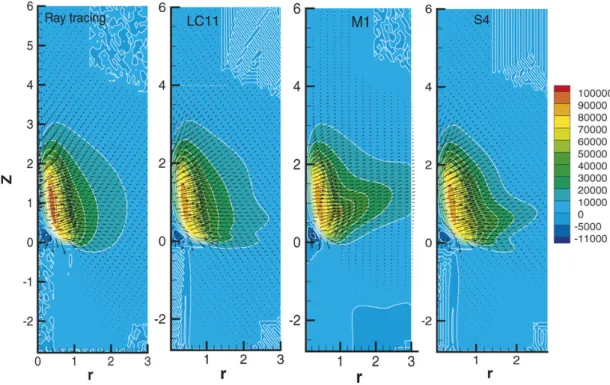
InFig. 10, two-dimensional contour plots of the radiative flux provide additional insight. As a remark, it is noted that all methods compute vanishing fluxes
Fig. 10. Contour plots of the radial component of the radiative flux (W/m2) along the centerline of the fire domain computed by, from left to right, ray tracing, DOM LC11, M1, and DOM S4.
inside the fuel pan and the wall (the interior zones are here visible, as for instance next to the chimney, in the upper right corner). The immersed boundary con-ditions, as used here to model this complex geometry, were found to be efficient even though an artificial absorption zone was found in the first cells of the pan in direct contact with the fire. There is no artificial
flux created below z= 0 and no heat travels through
the walls or the pan. All methods considered found flux vectors similar in direction, independent of the method used; the global direction 1 m from the cen-terline which is slightly tilted north east is found by the four methods considered here. Moreover, the ra-diation emitted from the hot regions and absorbed in the preheating cone can be seen.
Fig. 10 also illustrates a ray effect in both DOM
solutions at an elevation just above the pan at z =
0.1 m, evident by the sharp indentation in the con-tours of constant flux at radii larger than the pan,
r " 1 m, and stronger fluxes downward below the
pan level. The same effect could be seen previously in the profiles inFigs. 9e–9f. This effect is believed to be due to proximity to the fuel pan. Both DOM
methods suffer from this ray effect, although LC11
is significantly closer to the ray-tracing solution than S4, and is thus the more accurate solution technique.
On the other hand, the flux contours of M1 do not
contain the same sharp indentation nor strong down-ward fluxes below the pan elevation. This is believed
to be due to the M1 closure which, by
construc-tion, allows only one anisotropic direction at one
given location. As a result, a global, unique, and, as previously described, slightly tilted northeast di-rection is observed. This didi-rection is believed to be
due to the hot emitting region at r = 1 m. Along
this direction, the fluxes taken at a diameter away
from the fire begin to be overestimated by M1, as
seen previously in Figs. 9e–9f. A nozzle profile is
then formed due to the fact that this model does not limit sufficiently the fluxes in regions of strong anisotropy.
5. Conclusions
Six different methods were used to compute the ra-diative field of a synthetic 2-m, JP-8 pool fire,
includ-ing Monte Carlo, ray tracinclud-ing, DOM S4, DOM LC11,
DTM, and the M1 moment model. The M1 method
was applied for the first time to a combustion problem occurring in a complex three-dimensional geometry. Theoretically, this model has the lowest computa-tional cost of the six, since the direccomputa-tional integration is handled analytically with a model.
An angular resolution study has shown that a min-imum of approximately 50 angles inside and 350 an-gles outside the fire are needed to accurately compute radiation when a uniformly distributed set of angles is chosen. This choice of angles is not optimum, how-ever, and the number of angles needed can be reduced when an optimum quadrature is chosen. It was shown that these numbers can be reduced to 24 inside when
the S4 quadrature is chosen and to 100 outside when
the LC11 quadrature is chosen. Unfortunately, using
this many angles still results in a considerable compu-tational cost. It was also shown that if an insufficient angular distribution is used, significant changes to the time-dependent solution may occur. It is thus not pos-sible to accurately compute a time-accurate fire if the aforementioned angular requirements are not satis-fied.
The ray-tracing and Monte Carlo methods, which are the most accurate methods when their conver-gence is ensured, were used to compute reference so-lutions for the radiative source term and radiative flux fields. Results of both methods were shown to be es-sentially identical. Both of these methods, which need a large number of angles or a large realization sample, respectively, are too costly to be used for a three-dimensional time-dependent fire. It was found that inside the fire in isotropic regions all six methods give similar predictions of the radiative source term, which is needed for coupling with the hydrodynamics. Close to the fire, this term is underestimated by the S4and
M1 methods and overestimated by DTM, but the
de-viations were small enough that they would not affect the dynamic fire behavior. This demonstrates that the
M1 method gives results within the fire of sufficient
accuracy to be recommended for the computation of fire dynamics.
More discrepancies were found in the compari-son of the radiative flux. Inside the fire, all methods show agreement due to the isotropic conditions which exist inside the domain. However, outside the fire,
where anisotropic conditions exist, both the S4 and
M1methods inaccurately compute the flux. DOM S4
exhibited ray effects and the M1 method
overesti-mated the maximum flux by almost a factor of 2. These two methods are thus not effective if high ac-curacy is required for the heat flux to an object far
outside the fire. On the other hand, DOM LC11 and
DTM gave accurate solutions outside the fire.
Overall, it was shown that M1 results are most
similar to DOM S4 in the sense that its results are
accurate in regions where S4results are accurate, and
therefore, it is recommended that the M1 method be
considered for future combustion applications, since it is far less expensive computationally. The discrete transfer method was shown to give results similar to the ray-tracing reference solution, which was ex-pected; however, the reader is reminded that it is not
as efficient as DOM S4and M1. Finally, DOM LC11
gave results very close to the Monte Carlo and ray-tracing reference codes and is recommended for sit-uations where accuracy is more important than effi-ciency, especially in anisotropic regions of the com-putational domain.
Acknowledgments
Much of this work was performed during the Cen-ter for Turbulence Research 2004 Summer program. The authors express their sincerest gratitude to this institution and, in particular, to its director, Profes-sor Parviz Moin, who gave us the opportunity to ac-complish this work. The authors also especially thank Dr. Sheldon Tieszen of Sandia National Laboratories for his extensive technical discussions and encourage-ment. Kirk Jensen was supported by the Advanced Simulation and Computing Program of Sandia, a mul-tiprogram laboratory operated by Sandia Corporation, a Lockheed–Martin Company, for the United States Department of Energy’s National Nuclear Safety Ad-ministration under Contract DE-AC04-94AL85000.
References
[1] L.A. Gritzo, Y.R. Sivathanu, W. Gill, Combust. Sci. Technol. 84 (1998) 113.
[2] B. Porterie, J.-C. Loraud, Numer. Heat Transf. A 39 (2001) 139.
[3] B. Porterie, J.-C. Loraud, Numer. Heat Transf. A 39 (2001) 155.
[4] J.-F. Sacadura, J. Quant. Spectrosc. Radiat. Transfer 93 (2005) 5.
[5] S.R. Tieszen, Annu. Rev. Fluid Mech. 33 (2001) 33. [6] D. Drysdale, An Introduction to Fire Dynamics, second
ed., Wiley, 1999.
[7] P. Joulain, Proc. Combust. Inst. 27 (1998) 2691. [8] V. Novozhilov, Prog. Energy Combust. Sci. 27 (2001)
611.
[9] R. Koch, R. Becker, J. Quant. Spectrosc. Radiat. Trans-fer 84 (2004) 423.
[10] G.N. Minerbo, J. Quant. Spectrosc. Radiat. Transfer 20 (1978) 541.
[11] M.F. Modest, Radiative Heat Transfer, third ed., McGraw–Hill, 2003.
[12] R. Siegel, J. Howell, Thermal Radiation Heat Transfer, fourth ed., Taylor & Francis, New York/London, 2002. [13] D. Mihalas, B.W. Mihalas, Foundation of Radiation Hydrodynamics, Oxford Univ. Press, New York, 1984. [14] G.C. Pomraning, The Equations of Radiation
Thermo-dynamics, Pergamon, 1992.
[15] J. Holen, M. Brostrom, B.F. Magnussen, Proc. Com-bust. Inst. 23 (1990) 1677.
[16] A.L. Brown, T.K. Blanchat, in: ASME Summer Heat Transfer Conference, Las Vegas, HT2003-40249, 2003. [17] N.C. Markatos, M.R. Malin, G. Cox, Int. J. Heat Mass
Transf. 34 (1982) 181.
[18] N.W. Bressloff, J.B. Moss, P.A. Rubini, Proc. Combust. Inst. 26 (1996) 2371.
[19] P. Joulain, in: M. Curtat (Ed.), Proc. Int. Symp. Fire Safety Sci., vol. 6, Poitiers, 1999, p. 41.
[20] S.P. Burns, Int. Symp. Radiat. Transfer 2 (1997). [21] C.D. Moen, G.H. Evans, S.P. Domino, S.P. Burns,
Pro-ceeding of IMECE2002-33098, 2002.
[23] D. Levermore, J. Quant. Spectrosc. Radiat. Transfer 32 (1984) 149.
[24] J. Fort, Phys. A 243 (1997) 275.
[25] T.A. Brunner, J.P. Holloway, J. Quant. Spectrosc. Ra-diat. Transfer 69 (2001) 543.
[26] J.-F. Ripoll, J. Quant. Spectrosc. Radiat. Transfer 83 (2004) 493.
[27] J.J. Murphy, C.R. Shaddix, Combust. Sci. Technol. 178 (5) (2006) 865.
[28] S.R. Tieszen, et al., SAND Report No. SAND96-2607, Sandia National Laboratories, 1996.
[29] J.J. Murphy, C.R. Shaddix, Combust. Flame 143 (2003) 1.
[30] K.A. Jensen, J.M. Suo-Anttila, L.G. Blevins, submitted for publication.
[31] T.K. Blanchat, SAND Report SAND01-2227, Sandia National Laboratories, 2001.
[32] W.G. Houf, SAND Report SAND99-8254, Sandia Na-tional Laboratories, 1999.
[33] S.P. Kearney, in: Proc. ASME Int. Mechanical Engi-neering Congress and Exposition, 2001.
[34] S.C. Lee, C.L. Tien, Proc. Combust. Inst. 18 (1981) 1159.
[35] K.C. Smyth, C.R. Shaddix, Combust. Flame 107 (1996) 314.
[36] N.G. Shah, The Computation of Radiation Heat Trans-fer, Ph.D. thesis, University of London, 1979.
[37] F.C. Lockwood, N.G. Shah, Proc. Combust. Inst. 18 (1981) 1405.
[38] S. Chandrasekhar, Radiative Transfer, Clarendon, Ox-ford, 1950.
[39] J.Y. Murthy, S.R. Mathur, J. Thermophys. Heat Trans-fer 12 (3) (1998) 313.
[40] J. Ströhle, U. Schnell, K.R.G. Hein, in: Int. Conference on Heat Transfer, Antalya, vol. 3, 2001.
[41] D. Joseph, et al., Int. J. Therm. Sci. 44–9 (2005) 851. [42] P.J. Coelho, P. Perez, M. El Hafi, Numer. Heat Transfer
B 43 (2003) 425.
[43] P. Perez, et al., Numer. Heat Transfer B 47 (2005) 39. [44] J.R. Howell, Adv. Heat Transfer 5 (1968) 1.
[45] J.M. Hammersley, D.S. Handscomb, Monte Carlo Methods, Monographies Dunod, Dunod, Paris, 1967. [46] J.T. Farmer, J.R. Howell, in: Y. Bayazitloglu, et al.
(Eds.), Radiative Transfer: Current Research, vol. 276, ASME, 1994, p. 203.
[47] J.T. Farmer, J.R. Howell, Adv. Heat Transfer 31 (1998) 333.
[48] M. Cherkaoui, et al., J. Heat Transfer 118 (1996) 401.
[49] M. Cherkaoui, et al., J. Heat Transfer 120 (1998) 275. [50] A. de Lataillade, et al., J. Quant. Spectrosc. Radiat.
Transfer 74 (2002) 5.
[51] P. Perez, et al., in: Int. Conference in Central Europe on Computer Graphics, Visualization and Computer Vi-sion, vol. 10, 2002, p. 69.
[52] V. Eymet, et al., J. Quant. Spectrosc. Radiat. Transfer (2004), in press.
[53] J.-F. Ripoll, B. Dubroca, E. Audit, Transp. Theory Stat. Phys. 31 (4–6) (2002) 531.