Construction Methodologies for Implied Volatility Surfaces

(1)

Construction Methodologies for Implied Volatility Surfaces

Francesco Ruta

(2)

Abstract

This research paper will provide a kit of “everything that needs to be known” about volatility to anyone coming from any scholastic background. It will allow the reader to understand how to use the Heston and Stochastic Alpha Beta Rho (SABR) models through MATLAB and the Monte Carlo and Black-Scholes processes through Excel. Another objective is to bring into practical terms all the theoretical formulas and concepts and see which of the previously stated construction methodologies performs best under various circumstances.

There will firstly be an introduction to the concept of volatility. The importance of the implied volatility surface will then be shown and there will be explanations of the various construction methodologies for implied volatility surfaces, varying form local stochastic volatility models to Levy processes and parametric representations.

In the empirical experimentations section, the Heston, SABR and Monte Carlo models will be put at comparison and will be examined in terms of correctly portraying the market implied volatility surface and market option prices for five equities. There will additionally be an attempt to capture the dynamics of the implied volatility surface through the examination of how the market and models’ surfaces evolve throughout time.

We will see that the SABR model is the most appropriate construction methodology with respect to both esti-mating implied volatility surfaces and calibrating option prices among the three analysed throughout the empirical section. However, it must also be noted that better implied volatility estimation does not necessarily mean better option price calibration, and vice-versa. Lastly, a model that is more precise than the others does not guarantee that it is precise when compared to market data.

(3)

Special thanks to:

Professor Olivier Bossard, who has supervised my work throughout the entire development of this research paper

Leonardo Ruta, Teresa Catania, Nicoletta Ruta, Carlotta Ruta, Gabriele Bianchi, Ada Bianchi and Elisabeth Osmont d’Amilly for the support given throughout the evolution of this study

(4)

List of Figures

1 S&P’s realised vs. implied volatility, 1990 - 2010 1 _{. . . .} ₁₅

2 Volatility smile from Table 1, 1 year to maturity . . . 15

3 Volatility skew example . . . 16

4 Implied Volatility Surface developed on MATLAB 2 _{. . . .} ₁₇

5 Volatility Surface of Table 1 . . . 18

6 S&P Log returns 1990 to 19993 _{. . . .} ₂₂

7 Flat volatility surface of Table 1 . . . 28

8 Comparison of Heston and Heston-Nandi models4 _{. . . .} ₃₂

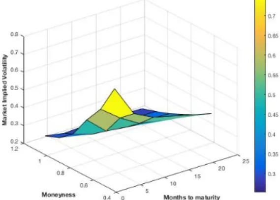
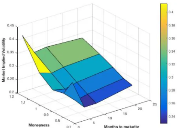
9 Citigroup Market Implied Volatility (%/100) - Call - 07/04/16 . . . 44

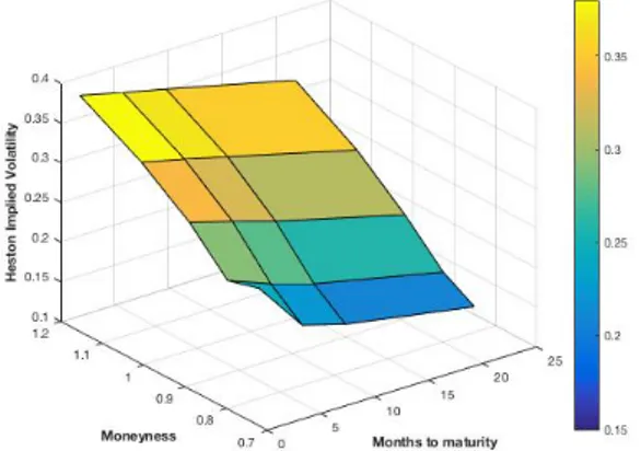
10 Citigroup Heston Implied Volatility (%/100) - Call - 07/04/16 . . . 44

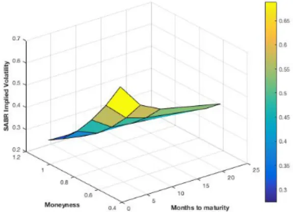
11 Citigroup SABR Implied Volatility (%/100) - Call - 07/04/16 . . . 45

12 Citigroup Monte Carlo Implied Volatility (%/100) - Call - 07/04/16 . . . 45

13 Citigroup Heston - Market price di↵erential ($) - Call - 07/04/16 . . . 45

14 Citigroup SABR - Market price di↵erential ($) - Call - 07/04/16 . . . 45

15 Citigroup Monte Carlo - Market price di↵erential ($) - Call - 07/04/16 . . . 45

16 Citigroup Market Implied Volatility (%/100) - Put - 07/04/16 . . . 46

17 Citigroup Heston Implied Volatility (%/100) - Put - 07/04/16 . . . 46

18 Citigroup SABR Implied Volatility (%/100) - Put - 07/04/16 . . . 46

19 Citigroup Monte Carlo Implied Volatility (%/100) - Put - 07/04/16 . . . 46

20 Citigroup Heston - Market price di↵erential ($) - Put - 07/04/16 . . . 47

21 Citigroup SABR - Market price di↵erential ($) - Put - 07/04/16 . . . 47

22 Citigroup Monte Carlo - Market price di↵erential ($) - Put - 07/04/16 . . . 47

(7)

65 Goldman Sachs Market Implied Volatility (%/100) - Call - 07/04/16 . . . 58

66 Goldman Sachs Heston Implied Volatility (%/100) - Call - 07/04/16 . . . 59

67 Goldman Sachs SABR Implied Volatility (%/100) - Call - 07/04/16 . . . 59

68 Goldman Sachs Monte Carlo Implied Volatility (%/100) - Call - 07/04/16 . . . 59

69 Goldman Sachs Heston - Market price di↵erential ($) - Call - 07/04/16 . . . 59

70 Goldman Sachs SABR - Market price di↵erential ($) - Call - 07/04/16 . . . 59

71 Goldman Sachs Monte Carlo - Market price di↵erential ($) - Call - 07/04/16 . . . 60

72 Goldman Sachs Market Implied Volatility (%/100) - Put - 07/04/16 . . . 60

73 Goldman Sachs Heston Implied Volatility (%/100) - Put - 07/04/16 . . . 60

74 Goldman Sachs SABR Implied Volatility (%/100) - Put - 07/04/16 . . . 60

75 Goldman Sachs Monte Carlo Implied Volatility (%/100) - Put - 07/04/16 . . . 61

76 Goldman Sachs Heston - Market price di↵erential ($) - Put - 07/04/16 . . . 61

77 Goldman Sachs SABR - Market price di↵erential ($) - Put - 07/04/16 . . . 61

78 Goldman Sachs Monte Carlo - Market price di↵erential ($) - Put - 07/04/16 . . . 61

(8)

121 Zions Bancorporation Market Implied Volatility (%/100) - Call - 07/04/16 . . . 72

122 Zions Bancorporation Heston Implied Volatility (%/100) - Call - 07/04/16 . . . 73

123 Zions Bancorporation SABR Implied Volatility (%/100) - Call - 07/04/16 . . . 73

124 Zions Bancorporation Monte Carlo Implied Volatility (%/100) - Call - 07/04/16 . . . 73

125 Zions Bancorporation Heston - Market price di↵erential ($) - Call - 07/04/16 . . . 73

126 Zions Bancorporation SABR - Market price di↵erential ($) - Call - 07/04/16 . . . 73

127 Zions Bancorporation Monte Carlo - Market price di↵erential ($) - Call - 07/04/16 . . . 74

128 Zions Bancorporation Market Implied Volatility (%/100) - Put - 07/04/16 . . . 74

129 Zions Bancorporation Heston Implied Volatility (%/100) - Put - 07/04/16 . . . 74

130 Zions Bancorporation SABR Implied Volatility (%/100) - Put - 07/04/16 . . . 74

131 Zions Bancorporation Monte Carlo Implied Volatility (%/100) - Put - 07/04/16 . . . 75

132 Zions Bancorporation Heston - Market price di↵erential ($) - Put - 07/04/16 . . . 75

133 Zions Bancorporation SABR - Market price di↵erential ($) - Put - 07/04/16 . . . 75

134 Zions Bancorporation Monte Carlo - Market price di↵erential ($) - Put - 07/04/16 . . . 75

(9)

177 Google Market Implied Volatility (%/100) - Call - 26/04/16 . . . 87

178 Google Heston Implied Volatility (%/100) - Call - 26/04/16 . . . 87

179 Google SABR Implied Volatility (%/100) - Call - 26/04/16 . . . 87

180 Google Monte Carlo Implied Volatility (%/100) - Call - 26/04/16 . . . 87

181 Google Heston - Market price di↵erential ($) - Call - 26/04/16 . . . 87

182 Google SABR - Market price di↵erential ($) - Call - 26/04/16 . . . 88

183 Google Monte Carlo - Market price di↵erential ($) - Call - 26/04/16 . . . 88

184 Google Market Implied Volatility (%/100) - Put - 26/04/16 . . . 88

185 Google Heston Implied Volatility (%/100) - Put - 26/04/16 . . . 88

186 Google SABR Implied Volatility (%/100) - Put - 26/04/16 . . . 89

187 Google Monte Carlo Implied Volatility (%/100) - Put - 26/04/16 . . . 89

188 Google Heston - Market price di↵erential ($) - Put - 26/04/16 . . . 89

189 Google SABR - Market price di↵erential ($) - Put - 26/04/16 . . . 89

190 Google Monte Carlo - Market price di↵erential ($) - Put - 26/04/16 . . . 89

219 Exxon Mobil Market Implied Volatility (%/100) - Call - 07/04/16 . . . 97

220 Exxon Mobil Heston Implied Volatility (%/100) - Call - 07/04/16 . . . 97

221 Exxon Mobil SABR Implied Volatility (%/100) - Call - 07/04/16 . . . 98

222 Exxon Mobil Monte Carlo Implied Volatility - Call - 07/04/16 . . . 98

(10)

224 Exxon Mobil SABR - Market price di↵erential ($) - Call - 07/04/16 . . . 98

225 Exxon Mobil Monte Carlo - Market price di↵erential ($) - Call - 07/04/16 . . . 98

226 Exxon Mobil Market Implied Volatility (%/100) - Put - 07/04/16 . . . 99

227 Exxon Mobil Heston Implied Volatility (%/100) - Put - 07/04/16 . . . 99

228 Exxon Mobil SABR Implied Volatility (%/100) - Put - 07/04/16 . . . 99

229 Exxon Mobil Monte Carlo Implied Volatility (%/100) - Put - 07/04/16 . . . 99

230 Exxon Mobil Heston - Market price di↵erential ($) - Put - 07/04/16 . . . 100

231 Exxon Mobil SABR - Market price di↵erential ($) - Put - 07/04/16 . . . 100

232 Exxon Mobil Monte Carlo - Market price di↵erential ($) - Put - 07/04/16 . . . 100

236 Exxon Mobil Monte Carlo Implied Volatility (%/100) - Call - 01/04/16 . . . 101

237 Exxon Mobil Heston - Market price di↵erential ($) - Call - 01/04/16 . . . 102

250 Exxon Mobil Monte Carlo Implied Volatility (%/100) - Call - 11/04/16 . . . 105

251 Exxon Mobil Heston - Market price di↵erential ($) - Call - 11/04/16 . . . 105

261 Citigroup Market Implied Volatility Surface (%/100) - Call - 28/03/16 . . . 108

262 Citigroup Heston Implied Volatility Surface (%/100) - Call - 28/03/16 . . . 108

263 Citigroup SABR Implied Volatility Surface (%/100) - Call - 28/03/16 . . . 109

264 Citigroup Monte Carlo Implied Volatility Surface (%/100) - Call - 28/03/16 . . . 109

265 Citigroup Market Implied Volatility Surface (%/100) - Put - 28/03/16 . . . 109

266 Citigroup Heston Implied Volatility Surface (%/100) - Put - 28/03/16 . . . 110

267 Citigroup SABR Implied Volatility Surface (%/100) - Put - 28/03/16 . . . 110

268 Citigroup Monte Carlo Implied Volatility Surface (%/100) - Put - 28/03/16 . . . 110

(11)

301 Data Call -5 to -1 1 . . . 134

302 Data Call -5 to -1 2 . . . 134

303 Data Call -5 to -1 3 . . . 134

304 Monte Carlo worksheet - Citigroup . . . 139

305 Heston and SABR Call -5 to -1 . . . 145

306 MC Call -5 to -1 . . . 146

(12)

List of Tables

1 Volatility Surface example . . . 17

2 Citigroup Mean of Implied Volatilities (%) - Call . . . 44

3 SABR Calibrated parameters - Call . . . 44

4 Citigroup Mean of Implied Volatilities (%) - Put . . . 46

5 SABR Calibrated parameters - Put . . . 46

18 Goldman Sachs Mean of Implied Volatilities (%) - Call . . . 58

20 Goldman Sachs Mean of Implied Volatilities (%) - Put . . . 60

34 Zions Bancorporation Mean of Implied Volatilities (%) - Call . . . 72

36 Zions Bancorporation Mean of Implied Volatilities (%) - Put . . . 74

50 Google Mean of Implied Volatilities (%) - Call . . . 86

52 Google Mean of Implied Volatilities (%) - Put . . . 88

(13)

62 Exxon Mobil Mean of Implied Volatilities (%) - Call . . . 97

64 Exxon Mobil Mean of Implied Volatilities (%) - Put . . . 99

74 Citigroup Implied Volatility Surface (%) - Call . . . 108

76 Citigroup Implied Volatility Surface - Put (%) . . . 109

82 Citigroup Mean of Implied Volatilities - Call(%) . . . 113

94 Implied volatility capture - Empirical Study 1 . . . 120

95 Prices di↵erentials summary - Empirical Study 1 . . . 120

(14)

1 Introduction: what is

volatil-ity?

1.1 Definition of volatility

Volatility takes various forms. It defines “how risky an investment is”, or also “the likelihood of a stock crashing”. We might also talk about stochastic volatil-ity, which is volatility that can take di↵erent values in option pricing models (and that hence is randomly dis-tributed). Realised volatility (or historical volatility) measures how the market has actually changed in the past. It “a statistical measure of the dispersion of re-turns for a given security or market index”5_.

It could as well be implied volatility, which is the volatility of an option that should persist shall various assumptions about the (the sensitivity of an option’s price to changes in the underlying’s price), (the first derivative of , or also the second derivative of the op-tion’s price with respect to the spot price), ⇢ (the sen-sitivity of an option’s price relative to interest rates), ✓ (the sensitivity of an option’s price relative to time to expiration of the option), strike price K and price of the derivative P are satisfied in the Black-Scholes model. It is an expectation of “how volatile the mar-ket can be in the future”6_{. It is “the} _{input into the}

BSM formula that generates the market observed op-tion price”7_{. Let us quickly remember the assumptions}

of the Black-Scholes model:

1. The asset’s asset price follows a Geometric Brow-nian Motion with and rf constant.

2. Short selling of securities is allowed. 3. No frictions.

4. No dividends.

5. No arbitrage opportunities. 6. Continuous markets.

7. r is constant for every maturity.8_.

When talking about implied volatility, it can be con-sidered as an alternative way of pricing a derivative. Traders often execute transactions based on their be-liefs of implied volatility. When implied volatility is relatively high, there are expectations of a big market movement. When it is low, the market (or better, the price of the specific derivative) is expected to remain relatively stable.

Commonly marked with a , which stands for stan-dard deviation, volatility is a key aspect of pricing options and, as we will see throughout this research paper, multiple models ave tried to capture the exac-titude of implied volatility of options with respect to the ✓ and the K of the option. Traders often base their

5_{http://www.investopedia.com/terms/v/volatility.asp} 6_{https://www.tradeking.com/education/options/} what-is-implied-volatility 7_{http://faculty.baruch.cuny.edu/lwu/9797/Lec8.pdf} 8_{http://www2.math.su.se/matstat/reports/seriec/} 2011/rep7/report.pdf

trades on implied volatility instead of on the option price itself.

There is a positive relationship between the volatil-ity of an option and its price. Indeed, the higher the volatility of an option, the higher the probability of that option finishing in-the-money.

1.2 Why is volatility so important?

As stated previously, there are di↵erent types of volatility. Throughout this research paper we will be focusing a lot on implied volatility, which is calcu-lated form the Black-Scholes-Merton model. But why use implied volatility instead of using option prices di-rectly when quoting? It is more straightforward to express a view with respect to implied volatility than with respect to option prices. Indeed, implied volatil-ity does not vary when there is a variation in the spot price and/or in the strike and/or in the option pre-mium. Therefore, implied volatility is not dependent upon intrinsic value; while option prices are. How-ever, the intrinsic value has no real information value. Implied volatility, additionally, “has the normal return distribution (Black-Scholes-Merton model) as a bench-mark”9_.

As an example, a call with 2 years to expiration, strike price $50 priced at $2.5 cannot really be com-pared to another call with 2 months to expiration, strike at $45 and priced at $3. However, if the first one has an implied volatility of 30% and the second one an implied volatility of 50%, the comparison is clearer.

Moreover, if options are quoted with respect to a positive implied volatility surface, the type 1 no-arbitrage conditions will be directly insured10_{, where}

the type 1 no-arbitrage condition is the no-arbitrage condition between European options of a predeter-mined strike and a predeterpredeter-mined maturity vs. the underlying cash11_.

Lastly, there is also the technological aspect to it: when there is no options order flow, there is no neces-sity to update the implied volatility surface as often as option prices12_.

1.3 What a↵ects volatility?

When there is a disequilibrium between demand and supply for an underlying, the implied volatility of the derivative changes too.

When there is very high demand, the price of the security rises, as well as its implied volatility. The opposite is true when there is excess supply, and the option becomes cheaper.

9_{Carr and Wu - A new simple approach for constructing} im-plied volatility surfaces. (2011)

10_Ibidem 11_Ibidem 12_Ibidem

(15)

The time value of a derivative is also a key factor determining the total implied volatility of the deriva-tive itself. Indeed, taking the example of an option, the longer is the time to expiration, the higher the chance that the price of the option has in order to vary throughout time, which means higher implied volatil-ity13_.

Lastly, the strike price K of an option is a vital aspect of determining how much volatility an option has. The closer the option’s price is to the strike price, the higher the volatility. Hence, at-the-money options have the highest implied volatilities.

1.4 Realised volatility vs.

Implied

volatility: empirical evidence

Figure 1: S&P’s realised vs. implied volatility,

1990 - 2010 14

As you can see, when the market is not in tur-moil, realised volatility is actually lower than implied volatility. The opposite is true when there are market crashes: see as examples the Russian and South East Asian crises of the late 90s and the Financial Crisis of 2008.

1.5 Volatility smiles, skews and the

volatility term structure

What models do traders use when pricing options? Do they really use the Black-Scholes-Merton model or do they use a slightly di↵erent version of it? Are mar-ket prices of options very di↵erent or close to those predicted by Black-Scholes-Merton? “Are the proba-bility distributions of asset prices really lognormally distributed?”15 _{In order to answer these questions, a}

13_{http://www.investopedia.com/terms/i/iv.asp} 14_{http://www.spvixviews.com/wp-content/uploads/}

2012/02/Exhibit-13-SP-500-Implied-Volatility-vs.-Subsequent-Realized-Volatility.jpg

15_{J. C. Hull - Options, Futures, and other Derivatives}

closer look at the concept of volatility smile has to be given.

The key takeaway is that traders use a modified ver-sion of the Black-Scholes-Merton: one where they allow volatility to be stochastic and dependent on K and ✓. Let us see how volatility smiles work for both equity and foreign currency options.

As stated previously, implied volatility is a function of both K and ✓. When implied volatility is a function of exclusively the strike price, we observe empirically either volatility smiles or volatility skews.

The first one consists of a curve for which deep in-the-money and deep out-of-in-the-money options have far higher implied volatilities than at-the-money options. An example of the volatility smile is that of FX options.

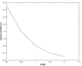
Figure 2: Volatility smile from Table 1, 1 year to maturity

The volatility skew is instead present in equity op-tions and equity index opop-tions markets. It consists of a downward sloping convex curve where implied volatil-ity decreases as the spot price of the options increases. Therefore, it is very low for in-the-money calls and out-of-the-money puts. An example is how in equity derivatives markets “extreme events” (such as a stock crash) are associated with higher implied volatilities, where a bearish market is riskier (and hence has higher volatility) than a bullish one16_.

Eighth Edition. (2012)

16_{L. Marroni, I. Perdomo - Pricing and Hedging Financial} Derivatives - A guide for Practitioners. (2014)

(16)

Figure 3: Volatility skew example

Reasons for a volatility skew include: leverage (stocks are more volatile at lower prices than higher ones); strong negative correlation between volatility and spot price moves; jumps in prices are more often seen downwards than upwards; supply and demand, as described previously. The volatility skew has been existing since the 1987 stock market crash17_.

We also need to take into account the T relation-ship, where T stands for time to maturity: the term structure of volatility plots implied volatility against T. Usually there is a direct relationship between the two variables. In other words, the lower is the time to expi-ration, the higher is the implied volatility. Therefore, the relationship between implied volatility and matu-rity can be thought of as a decreasing convex curve.

Thus, traders do not use the exact forms of the Black-Scholes-Merton model, because of various rea-sons: firstly they allow for the strike price and time to maturity to vary, and secondly they assume a distribu-tion for the asset (be it FX, equities, etc.) prices that is not lognormal.

While remembering that the implied volatility of Eu-ropean calls is the same as that of EuEu-ropean puts, let us recall the put-call parity18_:

p + S0e qT = c + Ke rT (1)

where q is the asset dividend yield. The put-call parity condition is true whatever the distribution of the asset price. Since put-call parity holds for the Black-Scholes model:

pBS+ S0e qT = cBS+ Ke rT (2)

In a no-arbitrage situation then we also have, for mar-ket prices:

pmkt+ S0e qT = cmkt+ Ke rT (3)

17_{http://faculty.baruch.cuny.edu/jgatheral/} impliedvolatilitysurface.pdf

18_{J. C. Hull - Options, Futures, and other Derivatives} Eighth Edition. (2012)

If we subtract the two equations, we have:

pBS pmkt= cBS cmkt (4)

Thus, if for example the implied volatility of a call option is 15%, then the Black-Scholes call price equals the market price of the call option when a volatility of 15% is used in the BSM model. Hence, given K and T, the correct volatility to use with the Black-Scholes-Merton model to price a European call should be the same as the one that is used to price a European put. Consequently the volatility smile is identical for both European calls and European puts, as well as the volatility term structure19_.

For foreign currency options, empirical evidence is that the lognormal distribution “understates the prob-ability of extreme movements in exchange rates”20 _.

The reasons for a smile in foreign currency options are that the volatility of the asset is not constant and that there are occasional jumps. The impact of these two characteristics of foreign currency options depends on T. As the time to maturity increases, the impact of non-constant volatility is more significant while the percentage impact on implied volatility is less so. On the other hand, the impact of jumps on prices and im-plied volatility becomes smaller and smaller as T aug-ments. Therefore, “the volatility smile becomes less pronounced as option maturity increases”21_.

When analysing equity options, because of what stated previously about leverage, the implied distri-bution is characterised by a fatter left tail and thin-ner right tail then the lognormal distribution. Indeed, as the stock price of an asset decreases, the leverage increases, making the stock more risky, with a conse-quent increase in volatility. Vice-versa, when a firm’s equity increases in value, the amount of leverage de-creases, making the stock less risky and thus a conse-quent decrease in volatility. Moreover, another expla-nation for the volatility skew in equity options is that since the October 1987 crash traders have become more scared of crashes, and they have since then adjusted for such probability when pricing options.

It is important to use K/S0instead of K simply when

plotting the volatility skew, because if there is a change in the equity price, then the volatility skew tends to move. This way there is much more stability in the skew and hence using such standardised measure allows to compare charts across various maturities and asset classes. Sometimes F0 is used instead of S0, since F0

is the “expected stock price on the option’s maturity date in a risk-neutral world”22_{. Other practitioners,}

such as Wu, use an even more standardised measure

19_Ibidem 20_Ibidem 21_Ibidem 22_Ibidem

(17)

for the moneyness of the option, which is Ln ⇣ K F0 ⌘ p T 23_,

where is the at-the-money volatility of the option. Other standardized measures include d1, d2and .

The volatility smile can also be defined as the rela-tionship between the implied volatility and the delta of the option, where usually the at-the-money option is a call option with a delta equal to 0.5 or a put option with a delta equal to -0.5.

The assumption of lognormality of the probability distribution of the underlying asset is made by the Black-Scholes-Merton model, but not by traders. The tails are fatter for FX options and the left tail of an equity option is fatter while its right tail is flatter when compared to the respective lognormal distributions. Fatter left tails are also said to exhibit leptokurtosis. For equity options, since the volatility smile is actually a skew, there is negative skewness in the distribution. Lastly, “for stock indexes the distributions are nega-tively skewed at both short and long horizons”24_.

Thus, non-flat implied volatility curves show that the distribution of returns of the underlying security is not at all normally distributed25_{. The reason why}

traders use volatility smiles is because “volatility smiles allow for nonlognormality”26_.

1.6 What is an implied volatility

sur-face?

An implied volatility surface plots the implied volatility of the option of a particular asset as a func-tion of strike price K and time to maturity ✓. There are two types of implied volatility surfaces: the one just described is an absolute implied volatility surface. If instead of using K, is used, then the result is a relative implied volatility surface27_.

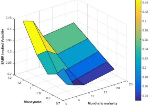
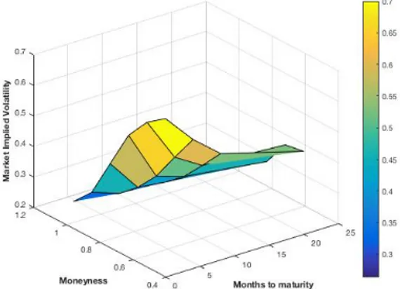
The volatility surface is a combination of the volatil-ity smile/skew and the term structure of volatilvolatil-ity, re-sulting in a 3-D graph, as Figure 4 shows. As stated previously, it is important to note that implied volatil-ity and time to maturvolatil-ity have a direct relationship when short-dated volatilities are historically low, since there are expectations for the volatilities to increase28_.

The opposite is true when short-dated volatilities are historically high, since there is an expectation for volatilities to decrease.

23_{http://faculty.baruch.cuny.edu/lwu/9797/Lec8.pdf} 24_Ibidem

25_Ibidem

26_{J. C. Hull - Options, Futures, and other Derivatives} Eighth Edition. (2012)

27_{https://en.wikipedia.org/wiki/Volatility smile} 28_{J. C. Hull - Options, Futures, and other Derivatives}

Eighth Edition. (2012)

Figure 4: Implied Volatility Surface developed

on MATLAB 29

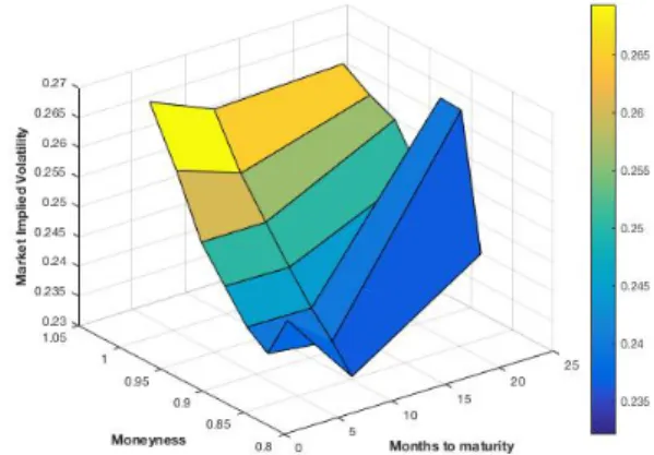
Table 1 shows an example of implied volatility sur-face data (with the respective graph, Figure 5).

Table 1: Volatility Surface example K/S0 0.90 0.95 1.00 1.05 1.10 1 month 14.2 13.0 12.0 13.1 14.5 3 month 14.0 13.0 12.0 13.1 14.2 6 month 14.1 13.3 12.5 13.4 14.3 1 year 14.7 14.0 13.5 14.0 14.8 2 year 15.0 14.4 14.0 14.5 15.1

Usually some of the data correspond to options for which trustworthy market prices can be retrieved. As a consequence, the implied volatilities for these specific prices and maturities are calculated directly, while the rest of the table is completed through interpolation. As an example, a 2 month option with a K/S0 ratio

of 1.10 would be interpreted by the financial engineer as having a value between 14.2 and 14.5; for example, using the average of the two numbers, 14.35%. This is the number that would be used in the Black-Scholes-Merton formula. So, “some points on a volatility sur-face for a particular asset can be estimated directly because they correspond to actively traded options”30_.

29 http://www.mathworks.com/matlabcentral/fileexchange/23316-volatility-surface/content/VolSurface.m

30_{http://www-2.rotman.utoronto.ca/ hull/} downloadablepublications/DHSPaperdraft7.pdf

(18)

Figure 5: Volatility Surface of Table 1

Certain financial engineers define the volatility smile as the relation between implied volatility and the fol-lowing _p1 TLn ⇣ K F0 ⌘

instead of that between the implied volatility and K31_.

The choosing of the model is fundamental to the shape of the volatility surface. If traders chose a model di↵erent to the Black-Scholes-Merton one, then, even with the shape of the smile changing, “the dollar prices that are quoted in the market would arguably not change appreciably”32_{. What has to be underlined is}

that “models have the most e↵ect on the pricing of derivatives when the derivatives do not trade actively in the market”33_{, such as certain exotic options.}

Volatility surfaces are used by traders to value Eu-ropean options when the price of such options cannot be directly observes in the market34_{. There is however}

a problem with exotic options such as barrier options, because, as Hull and Suo underline, the approach can-not be really extended to path-dependent exotic op-tions. Hence, some model risk exists.

Another use of the volatility surface is to hedge against changes in asset prices.

1.7 What does the implied volatility

surface communicate to us?

Let us firstly assume that the volatility surface is being built form European option prices. Let us also consider a butterfly strategy where we are:

1: long a call with strike K - K 2: long a call with strike K + K 3: short two calls with strike K

The value of the strategy, B0at t = 0 is the following:

31_{J. C. Hull - Options, Futures, and other Derivatives} Eighth Edition. (2012) 32_Ibidem 33_Ibidem 34_{http://www-2.rotman.utoronto.ca/ hull/} downloadablepublications/DHSPaperdraft7.pdf B0= e rTf (K, T )( K)2 (5)

where f(K,T) is the Probability Density Function of ST

at strike price K:

f (K, T )_{⇡ e}rTC(K K, T ) 2C(K, T ) ( K)2

+C(K + K, T )

( K)2 (6)

and if K goes towards 0, we have that f (K, T ) = erT@

2_C

@K2 (7)

“The volatility surface therefore gives the marginal risk-neutral distribution of the stock price, ST, for any

time, T”35_{. However, no information is given regarding}

the the joint distribution of the stock price at various periods T1, ..., Tn. This result makes sense as the

im-plied volatility surface is built from European option prices and these prices depend exclusively on the vari-ous marginal distributions of ST36.

1.8 Criteria for an e↵ective

representa-tion of the implied volatility surface

Three criteria are of fundamental importance if we want to represent properly the volatility surface:

1: Parsimony - the representation must have the minimum amount of information that is requested to have the entire implied volatility surface for all strike prices and times to maturity.

2: Consistency - the information included in the rep-resentation is constantly built along the times to matu-rity and strikes, so that interpolation or extrapolation of missing points is possible.

3: Intuitiveness - the information gives the user with an understandable view about the shape of the implied volatility surface, and “each piece of the information distinctly a↵ects one specific trait of the volatility sur-face”37

With the first criteria what is meant is that the representation is parsimonious if one can set up an interpolation-extrapolation scheme for both K and T, hence requiring only very few points as inputs. In the-ory, it should be hard to achieve, because for each ex-piry, a volatility smile has as many degrees of free-dom as strikes given. But empirically volatilities do not move independently of each other, and it can be assumed that there are only three degrees of freedom:

35_{http://www.columbia.edu/} mh2078/BlackScholesCtsTime.pdf 36_Ibidem

37 http://www.iasonltd.com/wp-content/uploads/2013/02/2b.pdf

(19)

level, slope and convexity. “In fact, as a principal com-ponent analysis can show, most of shape variations can be explained either by a parallel shift of the smile or by a tilt to the right or to the left or by a relative change of the wings with respect to the central strike”38_{. As}

a consequence, the minimum number of points needed at each time to maturity to portray the stylised move-ments is three, and they would consist in the volatil-ities for at-the-money options, out-of-the-money calls and out-of-the-money puts.

Moreover, these strike triplets, one for each expiry, must also be chosen in such a way that the resulting representation is consistent. Let us think of a very simple volatility surface with only two expiries: one week and ten years. For both expiries, one of the three strikes to choose may be set equal to the cur-rent price of the underlying asset (at-the-money spot). This choice is reasonable but not necessarily the best one. In fact, it would be better to replace the two at-the-money spot values with the forward prices at the two expiries, which can be viewed as expected values of the future underlying asset under suitable measures (the corresponding forward risk adjusted measures).

Things can even be worse for the other two points, since a meaningful selection criterion likely leads to dif-ferent values for the two expiries: two chosen strikes may convey a good amount of information regarding the smile for the one week expiry, but may be not so informative for the ten year expiry. In fact, what mat-ters (under a probabilistic point of view) is the rela-tive distance of a strike from the central one, possi-bly expressed in volatility units, which makes the cho-sen strikes, and their corresponding implied volatilities, comparable throughout the entire range of expiries. A meaningful distance measure is provided by the delta of an option (in absolute terms), since it is a com-mon indicator used in the market and it has the same signalling power as the relative distance from the at-the-money point (in units of total standard deviation). Finally, the representation is intuitive if directly ex-pressed in terms of three qualitative features of the surface, instead of three implied volatilities. These features, already mentioned above, are the level, the steepness and the convexity of the smile for each ma-turity. The level is correctly measured by the at-the money volatility.

Regarding the sets of expiry dates, a fixed number of maturities expressed as a fraction of years or as number of X months to maturity is the most intuitive choice to portray the implied volatility surface. Indeed, readers have an easier time by comparing times to maturity in the matrix and understand more intuitively which volatility corresponds to which strike and time to ma-turity39_.

38_Ibidem 39_Ibidem

(20)

2 No arbitrage conditions for

the implied volatility surface

We shall assume a dynamically complete mar-ket. If there is no arbitrage opportunity then there is an equivalent martingale measure char-acterised “by the risk neutral transition density of the underlying stochastic process denoted by ⇥(St, T|St, t, rt,⌧, t,⌧)”40, where Stis the price at time

t, T = t + ⌧ = expiry date, ⌧ time to expiration, rt,⌧

the risk-free rate and t,⌧ the dividend rate.

Moreover, we have that the valuation function of a European call is the following:

C(St, t, K, T, rt,⌧, t,⌧) = e rt,⌧⌧ ⇤ 1 Z 0 max(ST K, 0) ⇥(St, T|St, t, rt,⌧, t,⌧)dST (8)

Since the price function of a call option is a decreas-ing and convex function, derivdecreas-ing with respect to K, and together with the fact that ⇥ is both always pos-itive and integrable to one, one receives:

e rt,⌧⌧ _ @C(St, t, K, T, rt,⌧, t,⌧)

@K  0 (9)

which means that there is monotonicity.

2.1 No butterfly arbitrage

Convexity comes from di↵erentiating to the second degree with respect to the strike price (Breeden and Litzenberger, 1978): @2_C(S t, t, K, T, rt,⌧, t,⌧) @K = e rt,⌧⌧_⇥(S t, T|St, t, rt,⌧, t,⌧) 0 (10)

2.2 No calendar arbitrage

Let us also take into consideration that the call price is bounded by:

max(e t,⌧_S

t e rt,⌧⌧ K, 0)

 C(St, t, K, T, rt,⌧, t,⌧) e t,⌧⌧St (11)

2.3 Other remarks

All these constraints lead to nonlinear conditions for an arbitrage-free volatility surface. With the

assump-40_{M. R. Fengler - Arbitrage-Free Smoothing of the Implied} Volatility Surface. (2005)

tion of a strike-dependent volatility function, di↵eren-tiating twice the Black-Scholes formula yields:

⇥(K, T_|St, t) = e t,⌧⌧Stp⌧ ⌘( ¯d1) " 1 K2_ˆ⌧ + 2 ˆd1 K ˆp⌧ @ ˆ @K + ¯ d1d¯2 ˆ ✓_{@ ˆ} @K ◆2 + @ 2_ˆ @K2 # (12) “where ⌘ is the pdf of a standard normal value”41_.

If we are to adopt no-arbitrage conditions, then the implied volatility surface would need to assume that ⇥(K, T|St, t) 0 throughout all strikes and

maturi-ties. When considering T, there is only one weak con-straint, which consist in the prices of American calls for the same strikes to be non-decreasing. When there are no dividends involved, the same rule applies to Euro-pean calls42_{. However, the term structure of an implied}

volatility surface may be downward sloping as well. Kahale’ (2004) shows that, by treating the

zero-and zero-r case (even if his approach can be taken a step forward by having a deterministic, time-dependent rt and a dividend yield t “which are the

typical assumptions within the local volatility frame-work”43_{), we have the following argument (proven by}

Fengler in his thesis): “assume the existence of a deter-ministic, time-dependent interest rate rt and a

deter-ministic, time-dependent dividend yield t. If v2(k, ⌧i)

(which stands for our total variance) is a strictly in-creasing function for ⌧i = Ti t and i = 1,2, there is

no calendar arbitrage”44_.

So, an implied volatility surface gotten from con-vex call price functions that observe Ct(K2, T2) >

e

T2_R T1

tdt

Ct(K1, T1) or that is exclusively increasing in

the total variance, has no (calendar) arbitrage. Haug adds that skews should not be too steep at any given maturity, because otherwise there could be butterfly arbitrages. Additionally, “the term structure of the implied volatility cannot be too inverted”45_,

be-cause otherwise there would be calendar spread arbi-trages.

Let us now add Rebonato’s conditions that make sure of the existence of a risk-neutral density:

1: Market Conditions -we are in a complete market, with no taxes or transaction costs, no bid-ask spreads, short-sales are possible.

2: Traded instruments - possibility to trade both the underlying and plain-vanilla calls and put options for every single strike and time to maturity. There are also exists deterministic bonds and their income is determined by the risk-free rate r, and the payo↵s of

41_Ibidem 42_Ibidem 43_Ibidem 44_Ibidem

(21)

the options depend exclusively on the price evolution of the underlying asset until expiration46_.

The important equations to take into consideration in order to not have arbitrages are (9), (10) and (11).

Henstchel (2003) states that possible errors in data that can lead to arbitrage are the following: “bid-ask bounce, asynchronous pricing and finite quote preci-sion in option prices”47_.

2.4 If there is arbitrage

Even if arbitrage situations exist, they need not be removed necessarily from the data, and moreover im-posing the “monotonicity and convexity constraints in-troduces distortions in the observed process”48_.

However there are two situations where the data must be free of arbitrage: the first one is the “method of extraction of risk neutral densities”49_{. Here it is}

vi-tal that the data contains no arbitrage possibility so that the density extraction is appropriate. The other situation occurs through the model known as the “local volatility” one (Dupire’s smile model)50.

Arbitrage situations (real or “pseudo” arbitrage, the last one being potentially caused by prices mea-sured with errors and retrieved through interpola-tion/extrapolation) can be of major impact, “given the nonlinear transformations applied in calls prices”51_{. In}

density extractions in a risk-neutral world the arbi-trage situations in option prices can lead to very bad characteristics of the retrieved densities, “given that risk neutral is related to di↵erentiate the data two times, introducing large fluctuations. Arbitrage con-ditions can lead to the presence of negative probability points and multimodality in the extracted risk neutral density”52_.

In local volatility models, the arbitrages can condi-tion badly the local volatility, since estimacondi-tion of the local volatilities has the possibility to be based through the direct option quotations or in the potential volatil-ity surface if there are no-arbitrage possibilities. “The presence of arbitrage also a↵ects the stability proper-ties of the numerical methods used in the resolution of partial di↵erential equations present in local volatility equations”53_.

46_{M. Poletti Laurini - Imposing no-arbitrage conditions in} implied volatility surfaces using constrained smoothing splines (2007) 47_Ibidem 48_Ibidem 49_Ibidem 50_Ibidem 51_Ibidem 52_Ibidem 53_Ibidem