O
pen
A
rchive
T
OULOUSE
A
rchive
O
uverte (
OATAO
)
This is an author-deposited version published in :
http://oatao.univ-toulouse.fr/
Eprints ID : 19934
To link to this article : DOI:10.1063/1.4906153
URL :
http://dx.doi.org/10.1063/1.4906153
To cite this version : Esquivelzeta-Rabell, Francisco Martin and
Figueroa-Espinoza, Bernardo and Legendre, Dominique
and Salles,
Paulo A note on the onset of recirculation in a 2D Couette flow over a
wavy bottom. (2015) Physics of Fluids, vol. 27 (n° 1). pp.
014108/1-014108/14. ISSN 1070-6631
Any correspondence concerning this service should be sent to the repository
administrator:
[email protected]
OATAO is an open access repository that collects the work of Toulouse researchers and
makes it freely available over the web where possible.
A note on the onset of recirculation in a 2D Couette flow
over a wavy bottom
F. M. Esquivelzeta-Rabell,1 B. Figueroa-Espinoza,1,a) D. Legendre,2
and P. Salles1
1Laboratorio de Ingeniería y Procesos Costeros (LIPC), Universidad Nacional Autónoma de
México (UNAM), Puerto de Abrigo s/n, C.P. 97355 Sisal, Yucatán, México
2Institut de Mécanique des Fluides de Toulouse (IMFT), 2 Allée du Professeur Camille Soula,
31400 Toulouse, France
Laminar Couette flow over a fixed wavy surface was studied with direct numerical simulation in a 2D periodic numerical domain. The mesh was generated by a conformal transformation that sets horizontal flow at the top of the domain, where a constant velocity boundary condition is given. The bottom of the domain is a wavy sinusoidal surface of wave slope 2πa/λ. The combined effect of bottom shape, inertia, and viscosity was explored using different Reynolds numbers ( Re) and two dimen-sionless parameters in terms of channel width h, wavelength λ, and the amplitude of the wavy bottom a. Even if the Reynolds number was large, the simulations were not perturbed so the regime was always laminar. However, a recirculation appeared at the vicinity of the trough. The horizontal location of the eddy center was reported as a function of 2πa/λ and Reλ/h. The conditions for the onset of this recirculation were studied and compared with results from the literature. Two regimes can be clearly identified f rom t he n umerical r esults; a v iscous r egime w ith a w eak dependence between 2πa/λ and Reλ/h for small Reynolds numbers and an inertial regime with an exponential dependence between 2πa/λ and Reλ/h for large Reynolds numbers, which presents an approximate slope of −1/3. Almost all results collapse in one single curve that characterizes the phenomenon (with the exception of some points where the flow is confined due to a large λ/h ratio). C 2015 AIP Publishing LLC.
I. INTRODUCTION
The flow over wavy surfaces is relevant in many scientific and engineering applications, such as mass and heat exchangers (or reactors), that use corrugated surfaces.1Wavy surfaces are often found in problems related to deformable or granular media (e.g., wind-wave interactions in the ocean or sand dunes in the sea bottom, respectively). It is important to understand the basic mechanisms responsible for the complex behaviour observed in nature, such as the formation of dunes or ripples in the ocean bed like barchan dunes under the force of a shearing water flow (see experimental work of Groh et al.2). In particular, the shear stress and the normal pressure acting on the interface are
both responsible for the dynamic geometry modification in the field.3
Important phenomena such as boundary layer separation,4as well as transition to turbulence
are related to the occurrence of recirculation zones near solid boundaries. These recirculation zones appear as a consequence of adverse velocity profiles5 and is due to a combination of inertial, viscous, and geometrical effects. The following question arises: Which combination of these effects lead to the appearance of recirculation zones in a particular flow?
A 2D channel with a wavy bottom is a simple configuration that allows for the study of the aforementioned effects in many flow situations, and there are many theoretical and numerical pre-vious investigations that can provide information to validate and contribute to the understanding of fluid flow over a wavy surface.
Flow over wavy surfaces is a subject that has been widely investigated in the past; however, most of the studies reported in the literature have limitations when non-linear effects have to be considered. Miles6studied the generation of surface waves by shear flows solving a boundary value problem, obtaining results that agree with the observations in a qualitative way. Benjamin7produced an accurate linear theory for calculating the normal and tangential stresses on the boundary of a simple-harmonic wavy surface produced by shearing flows for stable laminar regime (and for turbu-lent flows considered as “pseudo-laminar” using the mean-velocity as velocity profile). The validity of the aforementioned theory is limited to large Reynolds numbers and small amplitudes, and it is assumed that the thickness of the boundary layer is much smaller than the wavelength. Benjamin7
neglected turbulence to study the phenomenon, and according to the linear theoretical analysis, the pressure and stresses over a wavy bottom can be defined in terms of sinusoidal functions.7(Eqs. 5.6 and 5.9 of his work).
Several studies have been carried out using channels with a wavy bottom. From the numerical point of view, Cherukat et al.8studied a turbulent flow over a solid train of waves using a spectral element Direct Numerical Simulation (DNS) technique. The authors observed interesting phenom-ena originating at the separation zone. A variety of flow patterns were observed to be in agreement with the observations reported in the literature. Sullivan et al.9also used DNS for the study of a
turbulent flow over idealized water waves represented by the lower wall of a 2D wavy channel using different wave slopes driven by a Couette flow. Their results agree with existing experiments and other simulations and show that the mean flow, velocity variances, pressure, and drag vertical mo-mentum fluxes are significantly influenced by the wave geometry and phase velocity c, normalized with the wave slope 2πa/λ, and the wave age c/u∗, where a is the amplitude of the wave, k = 2π/λ is the wave number, λ is the wavelength, u∗is the friction velocity defined as u∗= (τw/ρ), τwis the averaged shear stress over the wavy wall, and ρ is the density.
Pressure driven flows (Poiseuille) with wavy bottoms have also been studied in the literature. Nakayama and Sakio10 studied numerically, through DNS, a pressure driven flow over a wavy
bottom defined in terms of two modes of two-dimensional cosine waves, with different amplitudes and wavelengths at the lower boundary in order to explore the effects of filtering the small-scale fluctuations of the flow and the effects of smoothing of the boundary conditions on large eddy simu-lation (LES). Zhou et al.11studied Poiseuille flow using a perturbation technique for small wave
amplitudes and a finite element numerical code to investigate large perturbations for sinusoidal, triangular, and arched-shaped channels with a flat bottom. Sobey12has studied the Poiseuille flow using the triple deck theory in the asymptotic limit Re → ∞ using a first order approximation, obtaining that the critical(a/h) number for the onset of recirculation is (in our notation)
(a λ )
e
∼(Reh)−1/3, (1)
where Reh is defined in Eq. (7) and the subscript “e” refers to the onset of recirculation. Another
related problem studied by Floryan13is the linear stability analysis of a Couette flow over a wavy wall; the critical Re (which corresponds to the onset of streamwise vortices) was obtained as a function of the wave amplitude,
ln(Reg,cr) = −1.2801ln
(a h )
+ 2.9539, (2)
the author also established the behaviour of the wavenumber as a function of the amplitude for large Reynolds numbers (790. Re . 61 000).
In particular, the onset of recirculation in Couette flows over a wavy wall has been studied by some authors: for small Reynolds numbers, Scholle14has studied creeping flow using complex potentials based on Cauchy’s integral representation and Fourier series obtaining a set of algebraic equations, which were numerically solved, using a width-to-length ratio λ/h= 4 in order to obtain the wave-slope where the recirculation appears as 2π(a/λ)e≈ 0.4535.
Malevich et al.15investigated the onset of recirculation in terms of three dimensionless
num-bers: the Reynolds number Re (based on the wavelength), ε= a/h which describes the ratio be-tween the wave amplitude a and the channel height h, and b′= hk which represents the product
of channel height by the wave number k. The authors used the approach of perturbation expan-sions in terms of powers of a small ε and substituted the proposed solution into the full steady Navier–Stokes equations yielding a cascade of boundary value problems which were solved at each step in closed form. The authors also made an asymptotic analysis for large Reynolds numbers obtaining (in our notation)
(a h )
e
∼ Re−1/3e . (3)
Note resemblance with exponent of Eq. (1), obtained by Sobey12for Poiseuille flow.
Scholle et al.16studied the eddy genesis in Couette flow over a wavy bottom, using a finite
element formulation for the general case, and semi-analytically for the Stokes flow limit. The au-thors solved the problem for three specific cases: in the limit Re → 0, for small gaps, and large gaps, where the dimensionless mean gap is defined as hk= 2πh/λ. The same authors16also studied the difference between the position of the eddy center produced with the position of an eddy generated with Stokes flow using different combinations of the width-to-amplitude h/a and width-to-length λ/h ratios for cases where 0.77 < 2π/λ . 1.257.
Couette flows over non-sinusoidal walls have also been studied; Scholle17pointed out an inter-esting application of confined eddies to the tribology field, since these vortices may act as roller bearings.
The aim of this work is to establish the conditions for the onset of the recirculation in a flow over a wavy surface. DNS was used in order to test the geometrical conditions and Reynolds numbers where the onset of recirculation appears. Even though large Re were considered, the flow regime remained always laminar (The transition to the turbulent regime was left out of the scope of this investigation, for clarity.) Here, the term DNS is used to describe 2D full Navier Stokes simulations, which for the case of laminar flow at high Reynolds numbers do not present 3D fea-tures characteristic of turbulent flows. The 2D representation has proved to be pertinent in many situations, even for some turbulent flows where the mean flow has only one component (e.g., see Rao et al.18). The range of Re and geometrical parameters is extended to cases where non-linear
effects are important, in order to better understand the combined effects of inertia, viscosity, and geometrical parameters on the flow régime. In particular, we discus the effect of confinement on the onset of recirculation.
II. STATEMENT OF THE PROBLEM
The Couette flow over a wavy bottom is assumed incompressible, in the absence of body forces and without gravity.
The variables can be expressed in dimensionless form u= u U; (x ∗, y∗ ) =2π h (x, y); P = ph 2πU µ; t ∗= 2πUt h , (4)
where u is the velocity vector, x and y are the Cartesian coordinates, p is the pressure, and t is the time. The scale quantities are the velocity at the upper boundary U, the channel width h, and the dynamic viscosity µ.
The dimensionless Navier-Stokes equations become Reh
(∂u
∂t∗+ (u · ∇)u
)
= −∇P + ∇2u, (5)
together with the continuity equation,
where Reh represents the Reynolds number inspired in the channel width using µ as the dynamic
viscosity and ρ as the density. In order to compare results with literature, an alternate Reynolds number inspired in the wavelength Re is also defined,
Reh=
ρUh 2π µ; Re=
ρUλ
2π µ; (7)
boundary conditions are periodic,
u(0, y∗) = u(2π, y∗); P(0, y∗) = P(2π, y∗). (8) The velocity is imposed at north boundary,
u(y∗= 2πh/λ) = (1,0). (9)
The south boundary is a no-slip condition, u(y∗= acos(x∗
)) = (0, 0), (10)
and the initial condition u= u0(at time zero) throughout the domain is a linear (Couette) velocity
profile, note that there is no recirculation in this profile, u0= (u0,v0) = (y∗− 2πa cos (x∗ )/λ hk −2πa cos(x∗)/λ,0 ) . (11)
This initial condition (at t= 0) has the advantage to satisfy the boundary condition imposed at the entrance (x= 0), at the bottom (u = 0), and at the top of the domain (u = U). It also has the advantage to take much less running time to reach a quasi-stationary state than starting the simulation with an upper wall moving horizontally above a quiescent fluid. This initial condition is obviously not divergence free in the domain, but the divergence free condition is obtained at the end of the first time step. Due to the small value of the time step, the corresponding initial perturbation has no effect on the evolution of the solution to the steady state, and the computing time corresponding to the establishment of the Couette flow (diffusion time) is saved.
III. METHODOLOGY
The numerical code used in this study is called JADIM, and was developed at the Institute de Mécanique des Fluides de Toulouse (IMFT). The code can solve the 3D Navier–Stokes equations for incompressible and unsteady situations in terms of velocity–pressure variables. The discretiza-tion method is finite volumes, which is well adapted to properties conservadiscretiza-tion. Precision is second order in time and space (Runge–Kutta/Crank–Nicolson schemes) and the code has been used to successfully solve hydrodynamic and heat/mass transfer problems in the past.19–23
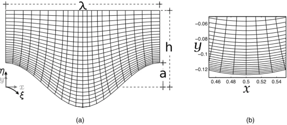
Boundary fitted grids were produced using a conformal transformation that maps a rectangular mesh into the geometry as illustrated in Fig.1(note that the resolution is not the one used in the simulations), where the south boundary represents a wavy surface of amplitude a. The transformed variables were taken from the conformal transformation used by Caponi et al.24expressed as series
expansions in terms of sinusoidal functions, given by Eqs. (12) and (13), x λ = ξ + ∞ n=1 bn n sin(nξ) cosh(n(ηT−η)) sinh(ηTη) , (12) y λ = η + b0− ∞ n=1 bn n cos(nξ) sinh(n(ηT −η)) sinh(ηTη) , (13)
where x and y represent the horizontal and vertical coordinates, respectively, λ is the wavelength, bn are constant coefficients, ξ and η are the (horizontal and vertical, respectively) transformed
variables that represent the curvilinear mesh.
Equations (12) and (13) were truncated to 25 terms. The mesh cell width was constant in the direction of ξ (horizontal). The cell height varied along the vertical direction η for y < 2λ with mesh refining near the wavy wall, and remained constant y > 2λ, with larger mesh cells at the top
FIG. 1. (a) Diagram of a mesh produced by conformal transformation (Eqs. (12) and (13)). (b) Zoom in the valley of the mesh (nx= 59 and ny = 84) used for the case where 2πa/λ = 0.8 and λ/h = 0.2.
of the mesh. The rate of change of the cell height is determined by S= ∆ηi
∆ηi+1, where ∆ηiand ∆ηi+1
are the height of a given cell and its upper neighbour, respectively. All simulations were run using S = 1.09, this rate of change has proved to be of no consequences in terms of numerical stability. A zoom in the valley of the grid used for the case 2πa/λ= 0.8 and λ/h = 0.2 is shown in Fig.1(b).
Note that the system is described by six parameters: U, µ, ρ, a, λ, and h. By applying Bucking-ham’s Pi-Theorem, only three non-dimensional parameter combinations remain: we have used in this study the Reynolds number Re (defined in Sec.I), the wave slope 2πa/λ, and the width-to-length ratio λ/h. The parameter ranges used in this study are shown in TableI. The value of λ/h infers on the confinement. When increasing λ/h confinement effects are expected to modify the flow.
Convergence tests were carried out for the wave slope 2πa/λ= 1.20, λ/h = 1, and Reynolds number Re= 5000/π using different number of nodes in both vertical and horizontal directions. The criterion used to find independence consists in obtaining the averaged bottom wall shear stress as a function of mesh resolution until we find almost identical results. Grid independence was found when the size of the cell closer to the wall was ∆xλgrid ≤ 1.668-2 and ∆yλgrid ≤ 2.60-4 at the crest
and∆xλgrid ≤ 1.712-2 ,∆yλgrid ≤ 3.48-3 at the valley, equivalent to nx = ny = 59.
IV. VALIDATION
The code has been extensively validated in the pass for flow in channel20and around spherical
body.19,21–23,25 In order to validate the code for the curvilinear system considered here, the results
from DNS were compared with the linear theory of Benjamin,7valid for large Reynolds numbers
and small wave slopes7(Eqs. 5.6 and 5.9 of his work were used to obtain τ
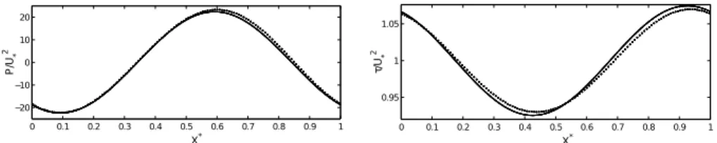
wt and Pwt). Figure2
shows the dimensionless shear stress and pressure for 2πa/λ= 0.01, λ/h = 1, and Re = 5000/π, both variables given as functions of the dimensionless length X= x/λ, and normalized by the mean friction velocity, given by
U∗=
τw/ρ. (14)
TABLE I. Range of parameters used in this study.
Parameter Range 2πa/λ 0.1 − 1.2 λ/h 0.01 − 2π Re 0−3142/π, 5000/π
FIG. 2. Wall normalized pressure and dimensionless shear stress for 2πa/λ= 0.01, λ/h = 1 and Re = 5000/π. Solid line: linear theory; dotted line: DNS.
Here, τwis the average shear stress along the wall,
τw=1
λ λ
0
τw(x)dx. (15)
The wall shear stress of the DNS was calculated from τwd= µ (∂u ξ ∂η ) η=0 , (16)
where uξis the component of the velocity parallel to the wall.
As a complimentary validation of the code, Fig.3shows the onset of recirculation for the limit Re → 0; the vertical axis corresponds to the parameter k(h − a), a dimensionless number used by Scholle et al.,16and the horizontal axis is the wave slope 2πa/λ. The solid line is the theoretical calculation of Scholle et al.,16 and the asterisks are the numerical simulations for small Reynolds number (Re ≤ 1) that corresponds to this work. Note that the regions below the solid curve repre-sent the conditions where recirculation does occur. The above validations give good agreement in the limiting cases of large Re and small 2πa/λ (linear theory), as well as for the creeping flow regime.
V. RESULTS AND DISCUSSION A. Numerical results
An example of the presence of eddies is shown in Fig.4, along with instantaneous streamlines. The flow is actually time-varying since the initial condition is inferred as the Couette flow given by Eq. (11), and the simulations stopped when a quasi-stationary state was reached. The criteria used
FIG. 3. Critical combination of geometric parameters k(a − h) and 2πa/λ (at which the eddies appear) at the limit Re → 0 for different values of λ
FIG. 4. Instantaneous streamlines of the flow field where 2πa/λ= 0.8, Re = 100, and λ/h = 0.1 at the scaled dimensionless time t∗h/λ ≈ 120: (a) near the bottom of the channel. (b) At the trough of the wavy surface.
to stop the simulations were based on the variation of the maximum velocity dvmaxthroughout the
domain between two time steps (usually reached before the scaled dimensionless time t∗h/λ ≈ 120).
We carried out the comparison between our criteria and the maximum variation of the wall shear stress (between two time steps) along the wavy bottom; the maximum variation in velocity is two orders of magnitude larger than the shear stress criteria.
The onset of recirculation is considered to happen when an adverse velocity profile appears along a line where ξ= constant (normal to the bottom of the channel, and vertical at the troughs and valleys). Our method to detect an adverse velocity profile consisted in analysing the whole lower row of cells along the bottom of the domain where η= constant in order to find the nodes where the velocity uξ is negative. We have verified that these criteria are equivalent to find the change of sign of the wall shear stress. It has been selected because it is more sensitive to the time convergence of the solution.
Fig.5characterizes the onset of recirculation, presenting the wave slope 2π(a/λ)eas a function
of the Reynolds numbers Ree. All the solid markers represent our numerical results for different
values of λ/h and divide the plane into the upper region, where recirculation occurs, and the lower region where there is no recirculation. Open markers represent the theory of Malevich et al.15,26
for different orders of approximation, which will be discussed later on a sub-section devoted to a comparison with the literature.
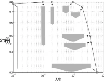
An alternative plane(Reλ/h)e vs. 2π(a/λ)e is proposed, as shown in Fig.6 where the wave
slope 2π(a/λ)eis presented as a function of the(Reλ/h)e. As expected, larger wave slopes require
smaller(Reλ/h)eto trigger the recirculation. The usefulness of using the selected combination of
dimensionless parameters is apparent from Fig.6: almost all the markers collapse to a single curve in terms of Reeλ/h. Moreover, in the limit of small (Reλ/h)e, the critical wave slope of recirculation
tends to be the same (2π(a/λ)e= 0.8) for almost all the values of λ/h ≤ 2. However, the solid
diamonds and circles seem to follow a different trend. This is the result of confinement (λ/h = 4 and
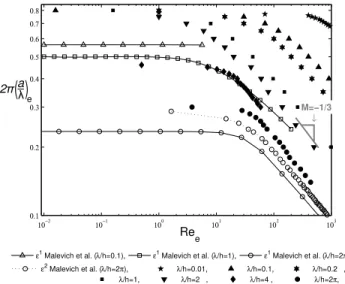
FIG. 5. Values of 2π(a/λ)ewhere the eddies appear as a function of Ree. Solid markers represent our simulations and the
FIG. 6. Values of 2π(a/λ)ewhere the eddies appear as a function of Reeλ/h. Dashed line represent the critical 2π(a/λ)e
found by Scholle14for small Reynolds numbers. Black horizontal line represent results of Scholle et al.16for 2πa/λ= π/25,
in the limit of large wavelengths and small channel width. The right side of dashed-dotted grey line represent a centrifugal instability in the flow according to Floryan.13The black dashed-dotted line represent the empirical Eq. (19).
λ/h = 2π): as stated by Scholle et al.,16the onset of recirculation is the result of a rich combination of physical effects (viscosity, inertia, and geometry). When confinement is dominant, in the limit of Ree→ 0, the onset of recirculation occurs at smaller wave slopes; otherwise, the wave slope seems
to reach a constant value (2π(a/λ)e≈ 0.8).
The effects of confinement can be also observed in Fig.7, where the wave slope 2π(a/λ)e is
presented in terms of λ/h for Ree→ 0: if λ/h increases, the onset of recirculation occurs at smaller
wave slopes. Such behaviour is consistent with that shown in Fig.3.
B. Presence of two regimes
In Fig.6, two flow regimes are apparent from the DNS results: a regime with a nearly linear dependence between 2π(a/λ)e and (Reλ/h)e in the range (0 ≤(Reλ/h)e. 1/2), dominated by
viscous effects and characterized by weak dependence on the wave slope 2πa/λ, and a second
regime with a clear exponential dependence between 2π(a/λ)e and(Reλ/h)e for(Reλ/h)e & 250,
where inertia dominates,
2π(a/λ)e= C(Reλ/h)eM, (17)
where M and C are the exponent and coefficient of the parameter Reeλ/h at the onset of the
recirculation, respectively, both dependent on λ/h (Fig. 5). In order to describe the behaviour of the phenomena excluding strong confinement (λ/h ≤ 2), we can set M ≃ 0 and C= 0.8 for the viscous regime ((Reλ/h)e ≤ 1/5) and M ≃ −0.33, respectively, and C ≃ 1.937 for the inertial
regime ((Reλ/h)e> 250).
C. Comparison with literature
In order to compare our results with the literature, let us first focus our attention in the results of Malevich et al.15(Fig. 8 of their work, ε
evs. Reewhere ε= a/h), which describe the problem
with the only assumption that ε is small. We present some of their results in Fig.5 for different order approximations in terms of ε (here, as in the figures of Malevich et al.,15,26we used the value
λ/h = 2π, according to a personal communication): Malevich theoretical results are presented as empty circles with different line styles. The continuous line is Malevich O(ε1) solution, and the dotted line is O(ε2
) approximation (note that solid markers are for our results and empty markers represent Malevich’s ones). It is shown that the second order approximation ε2of Malevich theory
is in qualitative agreement with our results in the limit of Ree→ 0 (if λ/h= 2π).
It is important to emphasize that the aforementioned results (Malevich) are not guaranteed to be valid in two regions: when 150 < Re < 600 due to precision problems26 (different orders of
approximation yields different results), and when 2π(a/λ)e > 2π(a/λ)c because above the critical
convergence value 2π(a/λ)c= (Re)−1/2the solution can bifurcate, so there are differences between
theory and numerical results.
Our numerical results were also compared with analytical expressions of first order approxima-tion of Malevich et al.15theory considering one case with confinement (λ/h= 2π) and two other
cases without it (λ/h= 1 and λ/h = 0.1). These last results are presented in Fig.5by empty circles, empty squares, and empty triangles, respectively. The aforementioned theoretical results do not collapse in one single curve in the limit of(Reλ/h)e→ 0, not even when there is no confinement.
As already mentioned, simulations show that confinement causes the onset of recirculation to occur at smaller wave slopes (for small Reynolds number, the wave slope decreases 2πa/λ < 0.8) when λ/h > 2, as shown in Figs.5and6, by solid diamonds (λ/h= 4) and solid circles (λ/h = 2π). This effect is consistent with the calculations of Scholle14 in the limit where Re
e→ 0 shown in
Fig.6as a dotted horizontal line[2π(a/λ)e= 0.4535] for λ/h = 4 and as empty circles for λ/h = 2π
in Fig.5.
The results of Scholle et al.16 for the limit of large wavelengths and small channel widths (confined cases that present large values of λ/h: 7.2 < λ/h < 15.2) for 2πa/λ= π/25 are pre-sented as a continuous black line in Fig.6. The largest value of λ/h presented by our results is λ/h = 2π. We can expect that slightly larger values of λ/h would practically reach Scholle limit 2π(a/λ)e= π/25, showing how sensitive the system is to confinement.
D. Large Reynolds numbers
The main results of the present work is obtained through the solution of Eqs. (5) and (6) using DNS. In order to validate the numerical trend (Eq. (17)) with a theoretical frame, the limit for large Reynolds numbers Re → ∞ and long length scales λ ≫ h is analysed in Appendix, and we show that in order to avoid recirculation in a wavy Couette flow we need
a λ ≪ ( λ hRe )−13 e . (18)
Note that we arrive to the same conclusion for symmetric perturbed Poiseuille flows (Eq. (1)) established by Sobey.12
The comparison between Eq. (18) and the slope of solid markers of Fig. 5 shows a good agreement between the triple deck theoretical description of the flow for big Reynolds numbers and also shows that it is not necessary to have long length scales λ ≫ h for presenting a −1/3 slope in Fig.5representation (as supposed by the approach presented in Appendix).
We also confirm the proportionality established by previous works for large Reynolds numbers; note the similarity between the value of exponent of Eq. (17) (M ≃ −0.33 at the inertial regime) and the exponents of Eq. (1) (for Poiseuille flow), Eq. (3) (for the Couette flow) and (A17) (comparing the slope of grey line and solid markers of Fig.5).
Even though the transition to the turbulent regime is not studied on this work, one should be cautious when interpreting the results of the onset of recirculation, since the flow can become unsta-ble for Reλ/h <(Reλ/h)eaccording to the linear stability analysis performed by Floryan13(where
the wave amplitude is supposed to be small a < 0.0349, according to the author’s Fig. 10). The critical value for the combination Reλ/h in the linear stability sense is shown as a dashed-dotted grey line on the lower right corner of Fig.6. The aforementioned line begins at Reλ/h ≈ 1380, and continues until Reλ/h ≈ 87 900. Note that the region to the right of that line shown as a gray poly-gon represents unstable behaviour in the sense of the appearance of unstable streamwise vortices. Out of the aforementioned unstable region, the 2D approximation can be expected to be valid.
E. General correlation
For practical purposes, it is possible to obtain a simple empirical expression that describes the onset of recirculation for unconfined cases (λ/h ≤ 2), incorporating the combination of useful dimensionless parameters used in the logarithmic representation of Fig.6,
2π(a/λ)e= * , ( 1 0.8 )3 + ( 1 1.937 )3( Reλ h ) e + -−13 . (19)
Equation (19) is represented in Fig.5as a black dashed-dotted line.
It is important to note that in the limit Re → 0, as well as Re → ∞, empirical expression (19) will be reduced to Eqs. (20) and (21), respectively. Note that the slope value M= −1/3 of empirical Eq. (19) is exactly the same than the slope of the theoretical frame of Eq. (A17).
F. Horizontal location of the eddy center
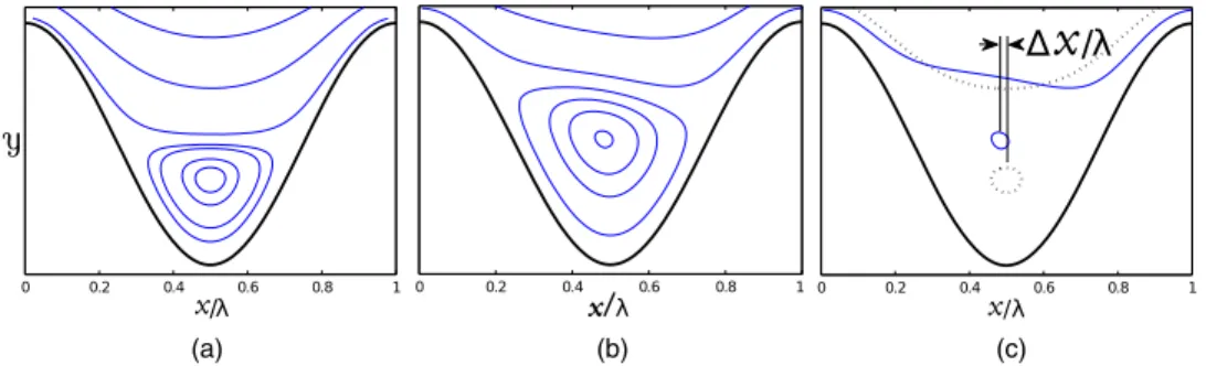
When there exists recirculation (above the critical curves in Fig.6), if the Reynolds number is increased, the eddy center moves horizontally upstream or downstream (∆X < 0 and ∆X > 0, respectively) as shown by Scholle et al.16 The authors reported that primary eddies (the first ap-pearing eddy) always appear at the trough. Moreover, it is important to note that in Scholle’s work, for all cases, the wave slope is between 0.77 < 2π(a/λ)Sc hol l e. 1.257 in his Fig. 10 and
2π(a/λ)Sc hol l e≈ 1.257 in his Fig. 12, which implies that the recirculation is present even in the
FIG. 8. Effect of increasing the Reynolds number in the eddy center location ∆x/λ using 2πa/λ = 1.2 and λ/h = 1. (a) Streamlines of an eddy produced with Stokes flow Reλ/h= 1, (b) eddies produced for the inertial regime Reλ/h = 90, (c) overlap of two previous cases illustrating the horizontal location of the eddy center ∆x/λ.
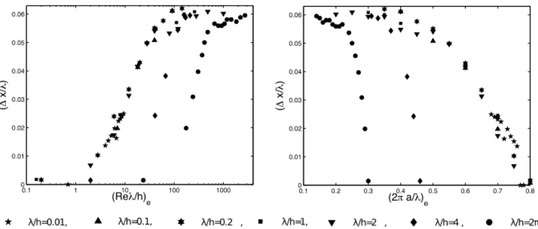
FIG. 9. Eddy center location ∆x/λ at critical conditions where the onset of recirculation occurs, as a function of(Reλ/h)e
at left and(2πa/λ)eto the right.
limit when Re → 0 due to the large wave slopes 2πa/λ compared with the critical value obtained by this study (2π(a/λ)e. 0.8, see Fig.6).
Considering that in most of the cases, the critical wave slope that produces the onset of re-circulation has equal or smaller wave slopes than the cases studied by Scholle et al.16 (2π
(a/λ)e
. 2π(a/λ)Sc hol l e), the locus of the created eddy ∆X/λ (see Fig.8(c)) at the onset of recirculation
is an interesting issue and is reported as a function of (Reλ/h)e and 2π(a/λ)e in Fig.9(left and
right side, respectively). It can be observed from the figure that the eddy forms at the center of the trough only when Rec→ 0. Otherwise, the recirculation forms always upstream (with respect to
the trough), as shown in Fig.9due to the dissymmetry induced by the non-linearity of the inertial contribution in the flow motion.
It can also be seen in Fig.9that all the geometrical configurations follow the same trend; as the parameter (Reλ/h)e increases, with a corresponding decrease on the parameter 2π(a/λ)e, the
position where the eddy is created moves upstream for all cases. The most confined cases (λ/h > 2) have smaller slopes with respect to(Reλ/h)eand steeper decrements with respect to 2π(a/λ)e.
VI. CONCLUSIONS
The onset of recirculation for a 2D Couette flow over a wavy boundary was investigated using a numerical simulation code that solves the full Navier-Stokes equations. Dimensional analysis leads to a characterization in terms of three dimensionless numbers: the Reynolds number, the width-to-length ratio λ/h, and the wave slope 2πa/λ.
The results were compared with various theoretical and numerical results from literature. The region in the 2πa/λ − Re space covered by this study is not restricted to a convergence criteria like the theory given by Malevich et al.15(as 2πa/λ= Re1/2) and compliments the results of Scholle14
(creeping flow) and Scholle et al.16in a range of Reynolds numbers where all viscous, geometrical, and inertial effects are important, resulting in a very rich combination of physical effects that cannot be described using only theoretical asymptotic techniques.
The use of the dimensionless number(Reλ/h)einstead of the Reynolds number allows for the
collapse of almost all results (with the exception of very confined configurations) in one single curve that characterizes the onset of recirculation in a Couette flow over a wavy bottom.
Two flow regimes were identified (excluding strong confinement): a “viscous” regime weakly dependent on the wave slope 2πa/λ, represented by
2π(a/λ)e≈ 0.8 ; (Reλ/h)e ≤
1
5, (20)
and an “inertial” regime described by
where M= −1/3 and C = 1.937 according our simulations. However, geometrical parameters play a significant role when confinement is important, causing the appearance of the recirculation at smaller wave slopes.
A remarkable agreement was founded between the slopes of the expressions obtained from numerical results and from the developed extended theory which states that recirculation can be avoided if
a/λ ≪ (Reλ/h)e− 1
3. (22)
The appearance of cross-stream eddies before the onset of instability13 suggests that they
interact with other fluid structures such as streamwise vortices and should be taken into account when studying important phenomena such as transition to turbulence or heat and mass transfer applications.
The present results can be useful in 3D situations if an analogous of the Squire theorem for the onset of recirculation could be verified15,27theoretically or numerically (3D simulations).
At critical conditions, the eddy forms at the center of the trough only when Rec→ 0;
other-wise, as the parameter (Reλ/h)e increases and the parameter 2π(a/λ)e decreases, the horizontal
location of the eddy creation moves upstream.
ACKNOWLEDGMENTS
The support of UNAM Research Grant No. PAPIIT IB100513 is gratefully acknowledged. The author F.M.E.R. thanks the Consejo Nacional de Ciencia y Tecnología (CONACYT) for the Ph.D. scholarship, UNAM for the academical formation, and IMFT for the internship.
APPENDIX: THEORETICAL APPROACH FOR LARGE REYNOLDS NUMBERS
This appendix describes the development of Sobey,12adapted to a wavy Couette flow. In turn, Sobey’s development is inspired by the work of Smith,28who studied Poiseuille flows at symmet-rically constricted or dilated pipes. Sobey12describes the behaviour of a Poiseuille flow in a long channel with boundary perturbations that vanish upstream and downstream.
If we assume that λ ≫ h, an asymptotic expansion of Eq. (5) is proposed using a scaled longitudinal variable X and suitably small parameters ϵ and σ defined by
ϵ = h λ; σ = a h; X = ϵ x ∗. (A1) Lower and upper boundaries take the next form (respectively),
y∗= σh cos(x∗
); y∗= 2πϵh. (A2)
As there is no external flow, the triple deck theory cannot be used in a straightforward way. It is possible to use the model of Smith28using an inviscid rotational core flow and viscous boundary layer regions near the walls.12The core of the flow can be represented as a perturbation of a flat Couette flow,
uv U0(y∗) + δU1(X, y∗), (A3)
v v ϵδV1(X, y∗), (A4)
pv P0+ PsP1(X, y∗), (A5)
where the capital letters U0= (y∗/(2πϵ),0) and P0represent velocity and the constant pressure for a
flat Couette steady flow, respectively. The capital letters U1, V1, and P1represents the pressure and
velocity perturbations due to the waviness. The δ and Psfactors are not determined yet.
Substituting Eqs. (A3)–(A5) into Eq. (5) and considering a steady state we get the x∗and y∗ momentum equations, respectively,
ϵδReh(U0U1X+ V1U0′) + ϵ δ 2Re
h(U1U1X+ V1U1y∗) = −ϵ PsP1X+ δU1y∗y∗+ ϵ2δU1X X, (A6)
ϵ2δRe
From Eq. (A6), we can see that the pressure perturbation will balance with the first inertial term, which leads to
Ps∼δReh. (A8)
The flow near the wall regions is assumed linear, and it can be represented by perturbation expan-sions using a scaled vertical variable y∗= σY,
uv σu0(X,Y ), (A9)
v v ϵσ2v
0(X,Y ), (A10)
pv P0+ Psp1(X,Y ). (A11)
If we substitute the Eqs. (A9)–(A11) into X momentum Eq. (A6), we get σ2Re
h(u0u0X+ v0v0Y) = −ϵ Psp1X+ σ−1uoY Y+ ϵ2σU0X X. (A12)
The boundary layer can be described by Eq. (A12), if σ2Re
hv σ−1 and ϵ Psv σ−1. (A13)
Combining Eqs. (A8) and (A13), we get
δ ∼ σ2, (A14)
and in combination with Eq. (A8) leads us to
Ps∼σ2Reh. (A15)
If we look into the order of magnitude of Eq. (A7), the only way to avoid vertical pressure changes at the core is if
ϵ2δRe
h≪ Ps. (A16)
If we substitute Eqs. (A14) and (A13) in the left and right side of Eq. (A16), respectively, we obtain the condition to avoid recirculation in wavy Couette flows: ϵ σ ≪ Re−
1 3 h . In other words a λ ≪ ( λ hRe )−13 . (A17)
1J. A. Stasiek, “Experimental studies of heat transfer and fluid flow across corrugated-undulated heat exchanger surfaces,” Int. J. Heat Mass Transfer41(6), 899–914 (1998).
2C. Groh, A. Wierschem, N. Aksel, I. Rehberg, and C. A. Kruelle, “Barchan dunes in two dimensions: Experimental tests
for minimal models,”Phys. Rev. E78(2), 021304 (2008).
3F. Charru, B. Andreotti, and P. Claudin, “Sand ripples and dunes,”Annu. Rev. Fluid Mech.45, 469–493 (2013). 4H. Schlichting and K. Gersten, Boundary-Layer Theory (Springer, 2000).
5L. Prandtl, Über flüssigkeitsbewegung bei sehr kleiner reibung. verh. III (Internationaler Mathematiker Kongress,
Heidelberg, Leipzig, 1904), pp. 484–491.
6J. W. Miles, “On the generation of surface waves by shear flows,”J. Fluid Mech.3(2), 185–204 (1957). 7T. B. Benjamin, “Shearing flow over a wavy boundary,”J. Fluid Mech.6(2), 161–205 (1959).
8P. Cherukat, Y. Na, T. J. Hanratty, and J. B. McLaughlin, “Direct numerical simulation of a fully developed turbulent flow
over a wavy wall,”Theor. Comput. Fluid Dyn.11(2), 109–134 (1998).
9P. P. Sullivan, J. C. McWilliams, and C.-H. Moeng, “Simulation of turbulent flow over idealized water waves,”J. Fluid Mech.404(1), 47–85 (2000).
10A. Nakayama and K. Sakio, “Simulation of flows over wavy rough boundaries,” in Annual Research Briefs (Center for
Turbulent Research, 2002), pp. 313–324.
11H. Zhou, R. J. Martinuzzi, R. E. Khayat, A. G. Straatman, and E. Abu-Ramadan, “Influence of wall shape on vortex formation
in modulated channel flow,”Phys. Fluids15, 3114–3133 (2003).
12I. J. Sobey, Introduction to Interactive Boundary Layer Theory (Oxford University Press, 2000).
13J. M. Floryan, “Centrifugal instability of Couette flow over a wavy wall,”Phys. Fluids14(1), 312–322 (2002). 14M. Scholle, “Creeping Couette flow over an undulated plate,”Arch. Appl. Mech.73(11–12), 823–840 (2004).
15A. E. Malevich, V. V. Mityushev, and P. M. Adler, “Couette flow in channels with wavy walls,”Acta Mech.197(3–4),
247–283 (2008).
16M. Scholle, A. Haas, N. Aksel, M. C. T. Wilson, H. M. Thompson, and P. H. Gaskell, “Eddy genesis and manipulation in
17M. Scholle, “Hydrodynamical modelling of lubricant friction between rough surfaces,”Tribol. Int.40(6), 1004–1011
(2007).
18K. S. Rao, J. C. Wyngaard, and O. R. Coté, “The structure of the two-dimensional internal boundary layer over a sudden
change of surface roughness,”J. Atmos. Sci.31(3), 738–746 (1974).
19J. Magnaudet, M. Rivero, and J. Fabre, “Accelerated flows past a rigid sphere or a spherical bubble. Part 1. Steady straining
flow,”J. Fluid Mech.284, 97–136 (1995).
20I. Calmet and J. Magnaudet, “Large-eddy simulation of high-Schmidt number mass transfer in a turbulent channel flow,” Phys. Fluids9, 438 (1997).
21D. Legendre and J. Magnaudet, “The lift force on a spherical bubble in a viscous linear shear flow,”J. Fluid Mech.368,
81–126 (1998).
22D. Legendre, J. Borée, and J. Magnaudet, “Thermal and dynamic evolution of a spherical bubble moving steadily in a
superheated or subcooled liquid,”Phys. Fluids10, 1256 (1998).
23B. Figueroa-Espinoza and D. Legendre, “Mass or heat transfer from spheroidal gas bubbles rising through a stationary
liquid,”Chem. Eng. Sci.65(23), 6296–6309 (2010).
24E. A. Caponi, B. Fornberg, D. D. Knight, J. W. McLean, P. G. Saffman, and H. C. Yuen, “Calculations of laminar viscous
flow over a moving wavy surface,”J. Fluid Mech.124, 347–362 (1982).
25Y. Hallez and D. Legendre, “Interaction between two spherical bubbles rising in a viscous liquid,”J. Fluid Mech.673,
406–431 (2011).
26V. V. Mityushev, personal communication (2014).
27H. B. Squire, “On the stability for three-dimensional disturbances of viscous fluid flow between parallel walls,”Proc. R. Soc. London, Ser. A142(847), 621–628 (1933).
28F. T. Smith, “Flow through constricted or dilated pipes and channels: Part 1,”Q. J. Mech. Appl. Math.29(3), 343–364