remote sensing
ISSN 2072-4292 www.mdpi.com/journal/remotesensing Article
An Adaptive Model to Monitor Chlorophyll-a in Inland Waters
in Southern Quebec Using Downscaled MODIS Imagery
Anas El-Alem 1,*, Karem Chokmani 1, Isabelle Laurion 1 and Sallah E. El-Adlouni 2
1 Centre Eau Terre Environnement, INRS, 490 De la Couronne Street, Québec, QC G1K 9A9,
Canada; E-Mails: karem.chokmani@ete.inrs.ca (K.C.); isabelle.laurion@ete.inrs.ca (I.L.)
2 Mathematics and Statistics Department, Moncton University, 18 Antonine-Maillet Avenue,
Moncton, NB E1A 3E9, Canada; E-Mail: salah-eddine.el.adlouni@umoncton.ca
* Author to whom correspondence should be addressed; E-Mail: anas.elalem@ete.inrs.ca; Tel.: +1-418-654-2570; Fax: +1-418-6542-6002.
Received: 15 January 2014; in revised form: 19 June 2014 / Accepted: 24 June 2014 / Published: 15 July 2014
Abstract: The purpose of this study is to assess the performance of an adaptive model (AM) in estimating chlorophyll-a concentration (Chl-a) in optically complex inland waters. Chl-a modeling using remote sensing data is usually based on a single model that generally follows an exponential function. The estimates produced by such models are relatively accurate at high Chl-a concentrations, but accuracy drops at low concentrations. Our objective was to develop an approach combining spectral response classification and three semi-empirical algorithms. The AM discriminates between three blooming classes (waters poorly, moderately, and highly loaded in Chl-a), with discrimination thresholds set using the classification and regression tree (CART) technique. The calibration of three specific estimators for each class was achieved using a multivariate stepwise regression. Compared to published models (Floating Algae Index, Kahru model, and APProach by ELimination) using the same data set, the AM provided better Chl-a concentration estimates (R2 of 0.96, relative RMSE of 23%, relative Bias of −2%, and a relative NASH criterion of 0.9). Moreover, the AM achieved an overall success rate of 67% in the estimation of blooming classes (corresponding to low, moderate, and high Chl-a concentration classes). This was done using an independent data set collected from 22 inland water bodies for the period 2007–2010 and for which the only information available was the blooming class.
Keywords: remote sensing; MODIS; inland waters; HABs; Chl-a; classification; CART; multivariate regression; stepwise
1. Introduction
Given its synoptic view, consistent recurrence, and capacity to provide information over a wide range of wavelengths, remote sensing has good potential to provide the data necessary to monitor harmful algal blooms (HAB). Bloom detection is possible through the bio-optical characteristics of the principal pigment in algae and cyanobacteria, chlorophyll-a (Chl-a), which is characterized by low reflectance in the red wavelengths and high reflectance in the near-infrared (NIR). This contrast makes it possible to estimate Chl-a concentration using bio-optical models that link inherent and apparent optical properties of water bodies [1]. For example, Landsat TM data have been used to retrieve Chl-a and total suspended solid (TSS) concentrations in Lake Kasumigaura using the neural network technique [2] and to assess phycocyanin concentrations in Lake Erie to study the temporal and spatial dynamics of cyanobacterial blooms [3]. In addition, data from the Advanced Very High Resolution Radiometer (AVHRR) have been used to assess the behavior of the main taxonomic groups of Lake Baikal phytoplankton as a function of ice conditions [4] and other water quality parameters [5,6]. Recently, QuickBird and MEdium Resolution Imaging Spectrometer (MERIS) data were used successfully to study cyanobacterial blooms in Lake Champlain [7]. Thus, many semi-analytical algorithms [2–4,8–21] and derived indices [22] are now available in the literature to retrieve Chl-a and phycocyanin concentrations in inland water bodies.
Although several models and approaches designed to model Chl-a in inland water bodies are now available in the literature, most assume that the concentrations of the whole range of optically active components in a water body can be modeled using the same function. However, this calibration function may be linear, exponential, or polynomial, depending on the relative concentrations of each component. Use of an inappropriate calibration function to estimate a given component may lead to over- or underestimates. This was clearly demonstrated by El-Alem et al. [23], who compared four exponential models used to estimate Chl-a at low-to-moderate and high concentrations. The accuracy of all four models significantly decreased at low concentrations [24]. Conversely, when low Chl-a concentrations were estimated using a linear [25,26] or polynomial [27] function, the results were more accurate. Moreover, it has recently been demonstrated that prior identification of the spectral type of inland waters significantly enhances the accuracy of Chl-a concentration estimates [28,29]. In addition, Yu et al. [29] have shown that estimation error can be reduced about 15 fold by using the appropriate spectral region to model low Chl-a concentrations.
Due to their one-day revisit time, MODIS images were privileged in this study. A short revisit time was considered desirable not only to enable us to collect enough data for model calibration and validation, but also to support eventual use of the technique in the context of risk management. The first two of the 36 MODIS bands in the red/NIR region are recorded at 250 m spatial resolution. The rest of the visible and shortwave infrared (SWIR) bands, which are more appropriate for the detection of Chl-a, colored dissolved organic matter (CDOM), and TSS, are recorded either at 500 m or 1 km
spatial resolution, making them unsuitable for monitoring algal blooms in small to medium-sized inland waters. However, the spatial resolution of MODIS bands 3–7 can be downscaled from 500 to 250 m using an approach developed at the Canadian Center for Remote Sensing (CCRS) by Trishchenko et al. [30]. In this manner, it is possible to acquire data from the first seven MODIS bands, originally designed for aerosol, cloud, and land applications, at 250 m spatial resolution, covering the visible, NIR, and SWIR parts of the spectrum.
The objective of the present study was to develop an adaptive model (AM) to estimate Chl-a concentration using MODIS data downscaled at 250 m spatial resolution and to evaluate its performance on a series of water bodies in southern Quebec, Canada. Performance of the AM was evaluated utilizing cross-validation using several statistical evaluation indices and a confusion matrix using an independent semi-quantitative database. We also used the same databases (continuous and ordinal) to compare performance of the AM to that of three other models originally developed to estimate Chl-a in inland waters (the Floating Algae Index (FAI), Kahru model, and APProach by ELimination (APPEL)) [13,22,24].
2. Materials and Methods 2.1. Study Area and in Situ Data
The study area, located in southern Quebec between latitudes 44° and 50° north and longitudes 67° and 80° west, contains 22 inland water bodies that are large enough to be investigated at 250 m spatial resolution and that have been monitored by the Ministère du Développement Durable, Environnement et Lutte contre les Changements Climatiques (MDDELCC) because of cyanobacterial bloom occurrence and recurrence as observed by the local volunteer monitoring network. These water bodies include the Choinière and Taureau reservoirs and Aylmer, Bouchette, Brome, Champlain, des Commissaires, Etchemin, Fréchette, Labrecque, Lovering, Mandeville, Maskinongé, Massawippi, Nairne, Ouareau, Perchaude, Pohénégamook, Roxton, Tortue, William, and Adélard lakes. These water bodies were used to calibrate and validate performance of the models (Figure 1).
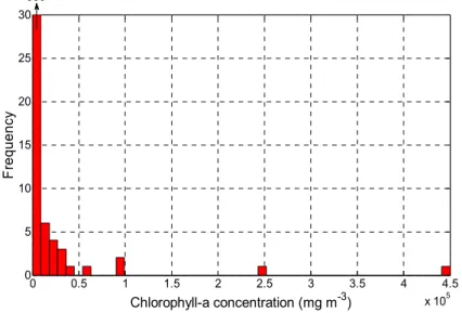
The calibration database of Chl-a concentrations was collected by the MDDELCC over nine years (2000–2008) at several sites located on four lakes (Brome, Champlain, Nairne, and William; Figure 2). A total of 363 samples were collected, with a minimum value of 0.52 mg Chl-a·m−3 (Nairne Lake, 2005), a maximum value of 450,000 mg·m−3 (Missisquoi Bay of Lake Champlain, 2001), an average of 3700 mg·m−3, and a median of 14 mg·m−3 (Figure 3). Chl-a concentration was quantified following the protocol of the Centre d’expertise en analyse environnementale du Québec (CEAEQ; 2012 [31]). Given the presence of clouds over some sampled sites and the poor quality of some images (fuzzy images or presence of artifacts), only 46 of these 363 samples could be used to calibrate the models. In this final data set, the Chl-a concentration varied from 2.7 (Nairne Lake, 2008) to 91,000 mg·m−3 (Missisquoi Bay of Lake Champlain, 2003).
Figure 1. Geographic location of the water bodies used for model calibration and validation.
Figure 3. Histogram of the frequency of chlorophyll-a values observed (complete data set, N = 363).
Three blooming classes were defined according to the thresholds used by the World Health Organization (WHO [32]) to characterize the quality of water bodies in relation to the hazard associated with water usage in the presence of algal blooms: the low Chl-a class corresponds to concentrations below 10 mg·m−3, the moderate class to concentrations between 10 and 50 mg·m−3, and the high class to concentrations above 50 mg·m−3. A second data set, used to validate the AM, was based on three cyanobacterial abundance classes: water bodies with cell densities lower than 20,000 cyanobacteria cells·mL−1 (assumed to be equivalent to 10 mg Chl-a·m−3 [32]), water bodies with densities between 20,000 and 100,000, and water bodies with densities higher than 100,000 cells·mL−1 (assumed to be equivalent to 50 mg·m−3). This data set was collected in the 22 water bodies listed above between 2007 and 2010 following the protocol of the CEAEQ (CEAEQ; 2012 [33]). For the same reasons as stated above, only 103 of the 677 samples collected were used to evaluate the performance of the AM.
2.2. MODIS Data
The remotely sensed data was obtained from the MODIS Level 1B product, available in HDF format on the NASA website (http://ladsweb.nascom.nasa.gov/data/search.html). The MODIS sensor is located on the TERRA platform of the NASA earth observation system. It operates across a wide spectrum, with 36 bands covering the region from 0.4 to 14.4 µm. Spatial resolution of the images varies from 250 m to 1 km. For this study, MODIS images collected on the same dates as the in situ samples were downloaded and pre-processed to calibrate the AM classifier and estimators. Given their higher spatial resolution, only the first seven MODIS bands were used in this study, enabling use of data from small lakes (but >2.25 km2). The first two bands were already at 250 m spatial resolution, while bands 3–7 were originally at 500 m (Table 1). The spatial resolution of the latter bands was downscaled to 250 m using an approach developed at the CCRS [30]. Two pre-processing steps were used in the downscaling process: (1) Translation of the data from 500 to 250 m spatial resolution using
0 0.5 1 1.5 2 2.5 3 3.5 4 4.5 x 10⁵ 0 5 10 15 20 25 30 Chlorophyll-a concentration (mg m-3) F req uenc y 350
adaptive regression and radiometric normalization as described by Trishchenko et al. [34]; and (2) re-projection of the images from the Sinusoidal to the Lambert Conformal Conic projection.
Table 1. Characteristics of the MODIS bands used in the present study. NIR = Near infrared; SWIR = Shortwave infrared; LCAB = Land/Cloud/Aerosol Boundaries; and LCAP = Land/Cloud/Aerosol Properties.
Primary Use Band Band Width (nm) Spatial Resolution(m) Spectral Regions
LCAB 1 620–670 250 Red 2 841–876 250 NIR LCAP 3 459–479 500 Blue 4 545–565 500 Green 5 1230–1250 500 NIR 6 1628–1652 500 SWIR 7 2105–2155 500 SWIR
Level 1B of the MODIS sensor contains a set of geo-located and calibrated data. For many applications, especially multi-temporal analyses, raw relative pixel values or digital image numbers have to be corrected for atmospheric effects and converted to spectral reflectance at the surface before the images are processed [35]. Improper atmospheric correction can lead to significant errors in the retrieved reflectance and affect the accuracy of the estimates [36]. Several atmospheric correction models have been developed, including the Simplified Model for Atmospheric Correction (SMAC [37]), Second Simulation of the Satellite Signal in the Solar Spectrum (6S [38]), Moderate-Resolution Atmospheric Transmittance and Radiance Code (MODTRAN [39]), ATmospheric CORrection (ATCOR [40]), Dark Object Subtraction (DOS [41]), and COSine Transmission for atmospheric correction (COST [42]). The DOS and COST models are widely used, as they rely entirely on image-based atmospheric corrections and provide reasonably accurate reflectance estimates, but accuracy is improved by the use of more sophisticated models that exploit in situ optical depth measurements and radiative transfer codes [42] to correct for both additive and multiplicative effects. A comparison study of three absolute atmospheric correction models, DOS, COST, and DOS4, produced similar results [41]. Reflectance was slightly improved, but the overall appearance was similar to the original image. The COST model was more effective in visible bands but less accurate in the NIR, particularly in humid conditions. On the other hand, a comparison analysis made by Norjamäki and Tokola [42] demonstrated that the RMSEr values for multi-temporal images decreased by an average of 6% using DOS, by 14% using SMAC, and by 15% using 6S, when compared to uncorrected images [43].
Figure 4 shows the signal recorded by the first seven MODIS bands during an algal bloom in Lake Champlain (19 September 2001) as adjusted using two different atmospheric correction models (SMAC and DOS) and the apparent reflectance (AR) model. The AR model performs a simple conversion from the digital numbers in the images to spectral reflectance at the surface, while the DOS model corrects the additive effects caused by haze, and the SMAC model additionally corrects multiplicative effects caused by ozone, water vapor, and aerosols. The comparison clearly shows that the reflectance estimated by the AR model is higher than that estimated by the SMAC and DOS models, especially for the first four bands (blue to NIR), and that the behavior of the return signal from the SMAC and DOS models is almost the same for all bands except the first one (blue). Since the AR
model does not correct for atmospheric effects and shorter wavelengths are easily scattered by atmospheric particles, the visible bands, particularly the blue one, were the most affected. The higher blue reflectance of the DOS model compared to SMAC was due to the huge sensitivity of this band to Rayleigh diffusion, which is mainly caused by water vapor and aerosols. The reflectance corrections performed by the SMAC model were closest to the spectral response of Chl-a, which is characterized by high absorption in the blue and red bands and high reflectance in the green and NIR bands. For these reasons, the SMAC model was chosen to correct the MODIS images. All pre-processing of images (down-scaling, re-projection, and atmospheric correction) was performed using an automatic tool developed by the CCRS [30].
Figure 4. Comparison of the MODIS signal from Lake Champlain during an algal bloom on 19 September 2001 with different atmospheric correction models.
2.3. Adaptive Model Parameterization
Parameterization of the AM was performed to exploit as much as possible of the spectral information captured by the MODIS sensors for a given water body. Analysis of the return signal for the low-to-moderate blooming class in the calibration data set shows reasonable correlation (R2 = 0.48; p-value < 0.0001) with the visible bands (triangle shape made by bands 1–3 on Figure 5A), whereas the return signal for high Chl-a shows good correlation (R2 = 0.95; p-value < 0.0001) with bands ranging from red to SWIR (polygon shapes made by bands 3–7 on Figure 5B). However, while the distinction between the spectral signature of high Chl-a and that of moderate-to-low Chl-a is obvious, the distinction between low Chl-a and moderate Chl-a is more complex (Figure 5A).
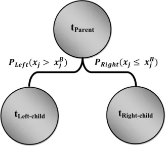
Created in the 1980s by Breiman [44], the Classification and Regression Tree (CART) method is widely used for classification and regression purposes. To build decision trees, CART uses a so-called learning sample, composed of a set of historical data with pre-assigned classes for all observations [44] and a set of spliting varaibles. These decision trees are then used to classify new data. Classification trees are built in accordance with a splitting rule, which splits learning samples into smaller groups of maximum homogeneity (Figure 6). The maximum homogeneity of child nodes is determined by the impurity function ( ( )), which can be calculated by either the Gini or the Towing splitting rule, and is equivalent to maximization of the change of impurity function ∆ ( ):
4690 555 645 859 1240 1640 2310 200 400 600 800 1000 1200 1400 Wavelength (nm) R e flectances * 1 0 -4 AR DOS SMAC
∆ ( ) = ( ) − − (1) where and are respectively the probabilities of right and left nodes. Consequently, at each node CART solves the following maximization problem:
argmax
, ,…,
( ) − −
(2) This enables CART to find the best value ( ) to split the (parent node) into (left node) and (right node) and maximize the change of impurity function ∆ ( ).
Figure 5. Spectral signature behaviour for three chlorophyll-a concentration classes: (A) low (<10 mg·m−3) and moderate (10–50 mg·m−3) concentrations combined; and (B) high
concentrations (>50 mg·m−3). Different colors represent the signature of individual samples.
Figure 6. The splitting algorithm of the Classification and Regression Tree (CART), where , , and are parent, left, and right nodes, is the splitting variable j, and is the best splitting value of the .
The CART method was applied to four variables derived from the spectral response of the first seven MODIS bands to classify the calibration data set into three blooming classes (water poorly,
t
ParenttLeft-child tRight-child
( ≤ )
moderately, and highly loaded in Chl-a). These variables were calculated from the surfaces (S) underneath the reflectance curves for (1) the visible bands (S ) ; (2) the green to NIR bands (S ); (3) the visible to NIR bands (S ); and (4) the red to SWIR bands (S ) using Equation (1).
=1
2 | ( ) × − ( ) × | (3)
where l is the number of MODIS bands and ( ) and are respectively the reflectance and wavelength absorption of the ith band.
Figure 7. Thresholds values (×106) used to distinguish between the three chlorophyll-a blooming classes using the classification and regression tree method (CART).
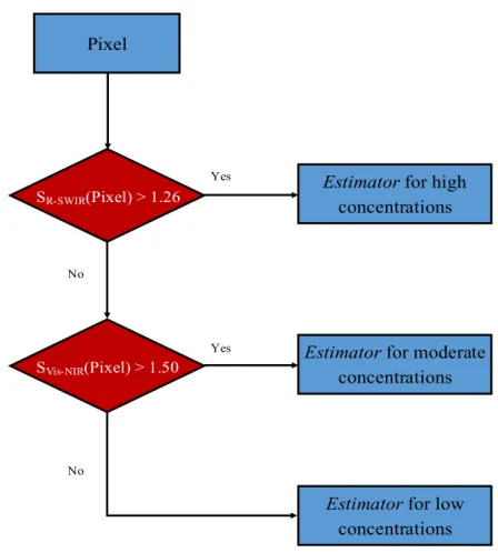
Before applying CART to the calibration database, we converted the continuous database into an ordinal one, i.e., the in situ measurements were classified into the three blooming classes defined above. The CART results (Figure 7) showed that (S ) and (S ) were the two best splitting variables, enabling us to calibrate the AM classifier. This classifier was thereafter used to split the calibration database into the three blooming classes. We then calibrated three different estimators, each specific to a given blooming class. The AM estimators were calibrated using a multivariate stepwise regression in which explanatory variables were chosen through an automatic procedure that usually followed a sequence of F-tests. We used the stepwise regression in the forward selection mode, starting with none of the variables in the model, testing them one by one, and including only the statistically
Pixel
SR-SWIR(Pixel) > 1.26
Estimator for moderate concentrations Estimator for high
concentrations
Estimator for low concentrations No No Yes Yes SVis-NIR(Pixel) > 1.50
significant ones [45]. All of the ratios and band subtractions possibly related to the bio-optical activity of Chl-a, and a range of algorithms widely used in the literature for inland water (as evaluated in [24]), were used as explanatory variables to train the three estimators. The mathematical expressions of the S and S variables and the three estimators are summarized in Table 2. The AM was thus structured in two steps: (1) determination of the blooming class of a given pixel based on the AM classifier; and (2) estimation of the Chl-a concentration of this pixel using the corresponding estimator for each predefined blooming class (Figure 7).
Table 2. Equations of the three calibrated models (or estimators) using a multivariate regression to estimate Chl-a concentration.
Blooming Classes Regression Estimators (Issued from Stepwise)
Low Chl-a [ − ] = . × × − . )
Moderate Chl-a [ − ] = ( . × ( ) . × × . )
High Chl-a [ − ] = ( . × . )
where is the calculated area underneath the reflectance signal curves from visible-to-NIR bands:
=| ( ) − ( )| + | ( ) − ( )| + | ( ) − ( )| + | ( ) − ( )|
For MODIS bands: = 645, = 859, =469, = 555, = 1240, = 1640 and = 2130 (nm)
and where APPEL is the APProach by Elimination model [1]:
= ( ) − [ ( ) − ( )] − [ ( ) − ( )] ∗ ( )
2.4. Accuracy Assessment and Validation Data
The performance of the AM and three other models (FAI [22], Kahru [13], and APPEL [24]) originally developed to estimate the Chl-a concentration of inland waters was evaluated using the cross-validation technique, in which a sample is temporarily removed from the calibration database and the remaining samples are then used as training data to estimate the value of the removed sample using the pre-calibrated model. This operation is then repeated for the whole database. Once all Chl-a measurements are estimated, the model’s performance can be evaluated using statistical indices such as the coefficient of determination (R2), relative root mean square error (RMSEr), relative bias
(BIASr), and relative NASH criterion (NASHr). The NASHr criterion evaluates the performance by comparing the estimated values to the in situ measurement average, producing a result that ranges between −∞ and 1.0 (inclusive). A negative NASH result means that it would be better to use the in situ measurement average than the model estimates, whereas values between 0.0 and 1.0 are generally viewed as acceptable levels of performance, and model performance is satisfactory for values higher than 0.8; the model is perfect for a NASHr = 1.0. The mathematical equations of the indices are as follows:
R = ∑ (M − M)(Es − Es)
∑ (M − M) ∑ (Es − Es)
BIASr =1 n Es − M M (5) RMSEr = 1 n Es − M ) M (6) NASHr = 1 −∑ M − Es M ∑ M − M M (7)
where n is the sample size, M and Es are measured and estimated values, and M and Es are the averages of measured and estimated values.
A second, independent, semi-qualitative database was also used to validate the performance of all models. This database, containing data on 22 water bodies monitored by the MDDELCC between 2007 and 2010, was composed of ordinal data that indicated only whether cell densities were lower than 20,000 cyanobacteria cells·mL−1 (assumed to be equivalent to 10 mg Chl-a·m−3 [32]), between 20,000 and 100,000 cells·mL−1, or higher than 100,000 cells·mL−1 (assumed to be equivalent to 50 mg·m−3). A confusion matrix was used to test the accuracy of the AM and the FAI, Kahru, and APPEL models. Omission and commission errors, success rates, and Kappa index (K) were calculated. The Kappa index was used to quantify concordance between the measured and the estimated Chl-a classes. Concordance is weak when the Kappa is negative, good for a Kappa that is positive and higher than 0.6, and excellent when the Kappa is above 0.8. Table 3 summarizes the parameters used in the confusion matrix as well as the Kappa index computation.
Table 3. Simplified diagram of the parameters used in the confusion matrix and to calculate the Kappa index: a and d are the number of well-classified values, b and c are the number of misclassified values, n1, n2 , n3, and n4 are respectively totals of a + b, c + d,
a + c, and b + d, N is the sample size, = , and = × × .
Measured
Estima
ted
TRUE FALSE Total Success Rate (%) Commission Error (%)
TRUE a b n1 (a/n1) (b/n1)
FALSE c d n2 (b/n2) (c/n2)
Total n3 n4 N
Success Rate (%) (a/n3) (d/n4)
Omission Error (%) (c/n3) (b/n4)
3. Results and Discussion 3.1. Calibration
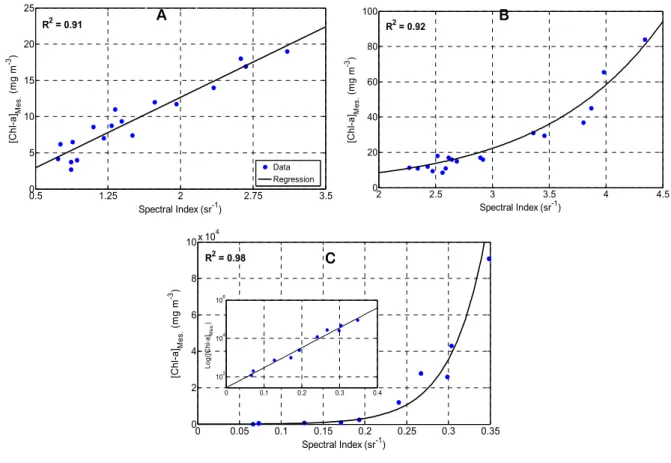
Eighteen samples served as the training set to calibrate the estimator for waters classified in the low Chl-a concentration class. The same number of samples was used to calibrate the moderate Chl-a estimator, and 10 samples were used to calibrate the high Chl-a estimator. The calculated spectral indices (existing approaches, subtractions, and band ratios) showed good correlation with in situ measurements for all three estimators. Low Chl-a concentrations were linearly correlated, while moderate and high Chl-a concentrations followed an exponential function (Figure 8). The determination coefficients (R2) were respectively 0.91, 0.92, and 0.98 for the three blooming classes.
The high correlation between in situ measurements and spectral indices (R2 > 0.91) for all three estimators illustrates the value of splitting the modeling workspace and using multivariate regressions. For all of the estimators, Chl-a estimation was limited to MODIS bands 1–4 or combinations of these bands, which contain the spectral regions most sensitive to the optical activity of the Chl-a pigment, i.e., high absorption in the blue (band-3) and red (band-1) and high reflectance in the green (band-4) and NIR (band-2). The stepwise regression maximized the information on the presence of Chl-a and minimized the mis-modeling of this pigment at the expense of other optically active components, such as TSS or dissolved organic matter (DOM), which exhibit different spectral absorption and reflectance signatures.
The explanatory variable selected by the stepwise regression for low blooming conditions, characterized by clear, non-turbid water, was S , which is mostly controlled by the visible part of the spectrum, consistent with the assumption that waters with low-to-moderate Chl-a are highly influenced by the bio-optical activity of the Chl-a pigment. S was also the variable selected by the CART method to discriminate between waters poorly and moderately loaded in Chl-a (Figure 7). High phytoplankton biomass, on the other hand, is known to generate turbid waters, which significantly reduce water molecule absorption in the red–NIR part of the spectrum [13]. This explains why the APPEL model, which depends entirely on NIR band reflectance to estimate Chl-a concentrations, was the best predictor for waters highly loaded in Chl-a. The transition class of waters moderately loaded in Chl-a would logically be influenced by both Chl-a bio-optical activity and turbidity. The explanatory variables selected by the stepwise regression for these waters supported this supposition. The Chl-a variance was explained by two orthogonal variables, S (sensitive to Chl-a activity) and R(λ ) (sensitive to turbidity), with most of the variance explained by S (p-value < 0.0001). The two variables did not show any collinearity (for both variables the variance inflation factor was equal to 1.5, which is <10, the threshold usually used to report collinearity issues).
Figure 8. Results of multivariate regression adjustments between the measured chlorophyll-a concentrations and the return signals of MODIS images for the three blooming classes: (A) Low; (B) Moderate; (C) High Chl-a concentrations. The scale of the y-axis in the insert is logarithmic to better illustrate the correlation.
3.2. Evaluation of Estimators
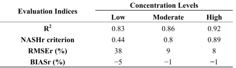
The performance of the three estimators was satisfactory and increased with higher Chl-a concentrations (Table 4). The results for the NASHr criterion demonstrate that the calibrated estimators are robust, in particular for moderate (NASHr = 0.8) and high (NASHr = 0.89) Chl-a concentrations. This is not surprising, as the mathematical expressions of the estimators for waters moderately and highly loaded in Chl-a are mainly based on the red-to-NIR bands, for which Chl-a reflectance is at its maximum, as shown in Figures 3–20 of Mackie (2010; [46]). Chl-a and water pixels are easily distinguished since water reaches its maximum absorption in this part of spectrum. The RMSEr results support the above findings, with a clear decrease in error for moderate and high Chl-a concentrations. The estimator for waters poorly loaded in Chl-a seems to overestimate the concentrations by 5%, while the estimators for moderate to high Chl-a concentrations are almost unbiased (BIASr = −1%). 0.5 1.25 2 2.75 3.5 0 5 10 15 20 25 Spectral Index (sr-1) [C h l-a ]Me s. (m g m -3) Data Regression R2 = 0.91 2 2.5 3 3.5 4 4.5 0 20 40 60 80 100 Spectral Index (sr-1) [C h l-a ]Me s. (m g m -3) R2 = 0.92 0 0.05 0.1 0.15 0.2 0.25 0.3 0.35 0 2 4 6 8 10 x 10 4 Spectral Index (sr-1) [C h l-a ]Me s. (m g m -3) 0 0.1 0.2 0.3 0.4 102 104 106 Log( [C hl -a]Mes. ) R2 = 0.98 A B C
Table 4. Evaluation of the three models (estimators) using cross-validation technique.
Evaluation Indices Concentration Levels
Low Moderate High
R2 0.83 0.86 0.92
NASHr criterion 0.44 0.8 0.89
RMSEr (%) 38 9 8
BIASr (%) −5 −1 −1
The relatively lower performance of the estimator for low Chl-a can be explained by the fact that its explanatory variable is mostly composed of bands located in the visible part of spectrum. Since the MODIS bands of higher resolution (at 250 m and at 500 m downscaled to 250 m spatial resolution) were designed for land, cloud, and atmosphere applications, they are not centered on Chl-a absorption and reflection peaks. Moreover, due to the low reflectance of water with low Chl-a concentrations, the return signal is more likely to be disturbed by noise caused by atmospheric particles, the reflectance of other optically active components present in the water (e.g., DOM), and the downscaling process, which can lead to the loss of up to 23% of the original MODIS signal [24].
3.3. Evaluation of the Adaptive Model: Cross-Validation
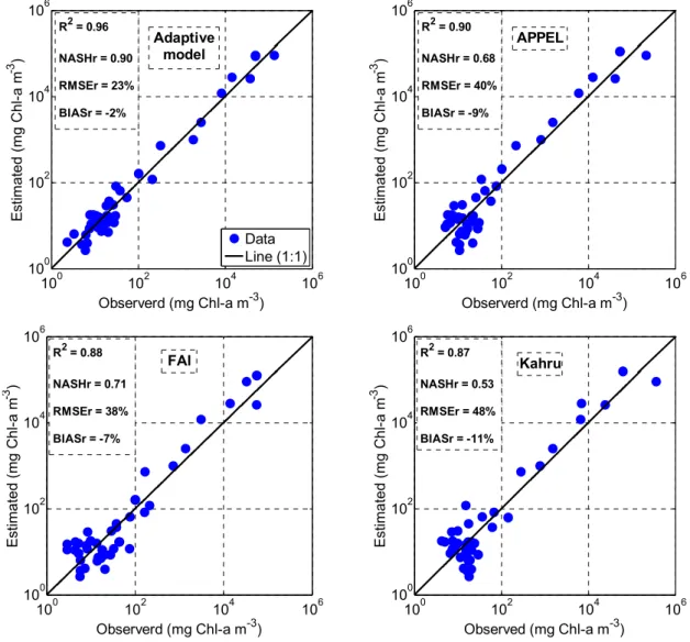
The performance of the AM, FAI, Kahru, and APPEL models was evaluated using a cross-validation based on the same database. Figure 9 shows the Chl-a estimated by the four models as a function of the observed Chl-a (measured in situ by the MDDELCC), along with the model performance indices. The figure clearly shows that the AM performed the best (R2 = 0.96, NASHr = 0.9, and RMSEr = 23%), followed by the APPEL and FAI models with almost identical performance, while the Kahru model performed the least well. However, the overall performance of the three comparison models (FAI, Kahru, and APPEL) was quite similar. The figure also demonstrates that the dispersion of values is well distributed with respect to the 1:1 line, highlighting the robustness of the models even at their extremities.
However, although the performance of all the models is satisfactory, it is clear that they are strongest when addressing high concentration values. In the context of timely intervention to manage risk and protect human and animal health, water bodies already affected by HAB are less interesting to monitor than relatively healthy waters with the potential to develop algal blooms and be exposed to eutrophication. When the performance of the models at moderate-to-low concentrations (<50 mg Chl-a mg−3, established by WHO as the threshold for declaring a HAB situation; Figure 10) is examined, only the AM provides acceptable estimates (R2 = 0.56 and NASHr = 0.24); the performance of the other three models was significantly lower, with negative NASHr values indicating that the measured Chl-a average were better predictors than the model estimates.
Figure 9. Chlorophyll-a concentration estimated from the four models compared to in situ measurements for the complete database, with model performance indices.
Figure 10. Chlorophyll-a concentration estimated from the four models compared to in situ measurements for the database using only values <50 mg Chl-a m−3.
100 102 104 106 100 102 104 106 Observerd (mg Chl-a m-3) E sti m at ed (m g Chl -a m -3 ) Data Line (1:1) Adaptive model R2 = 0.96 NASHr = 0.90 RMSEr = 23% BIASr = -2% 100 102 104 106 100 102 104 106 Observerd (mg Chl-a m-3) E sti m at ed (m g Chl -a m -3 ) APPEL R2 = 0.90 NASHr = 0.68 RMSEr = 40% BIASr = -9% 100 102 104 106 100 102 104 106 Observerd (mg Chl-a m-3) E st imated ( m g C hl -a m -3 ) R2 = 0.88 NASHr = 0.71 RMSEr = 38% BIASr = -7% FAI 100 102 104 106 100 102 104 106 Observed (mg Chl-a m-3) E st imated ( m g C hl -a m -3 ) R2 = 0.87 NASHr = 0.53 RMSEr = 48% BIASr = -11% Kahru 0 20 40 60 0 10 20 30 40 50 60 Observerd (mg Chl-a m-3) E st im at ed ( m g C h l-a m -3 ) Data Line (1:1) R2 = 0.56 NASHr = 0.24 RMSEr = 59% BIASr = -15% Adaptive model 0 20 40 60 0 10 20 30 40 50 60 Observerd (mg Chl-a m-3) E st im a te d ( m g C h l-a m -3 ) R2 = 0.14 NASHr = -2.25 RMSEr = 129% BIASr = -53% APPEL
Figure 10. Cont.
The above results indicate that partitioning the solution space into blooming classes increased the accuracy of Chl-a estimates, with estimators able to explain from 91% to 98% of the Chl-a variance (Figure 8C). Using an adequate calibration function for each blooming class (linear for low Chl-a and exponential for moderate-to-high Chl-a) specifically helped to improve the estimation of moderate-to-low Chl-a concentrations, which were problematic when applying the FAI, Kahru, and APPEL models. The AM error (RMSEr) was 200%–250% lower compared to the other models, and its systematic error (BIASr) was 300%–450% lower.
3.4. Validation by Independent Data
Tables 5–8 show the confusion matrix results for the AM, APPEL, FAI, and Kahru models. The AM performed the best (global success = 67% and Kappa index = 0.51), followed by the APPEL and FAI models, while the Kahru model performed the worst. From this analysis, we can see that estimating Chl-a at high concentrations was not problematic for any of the models, with commission errors of 17%, 18%, 18%, and 12% for the four models, respectively. On the other hand, the commission and omission errors were clearly higher for the APPEL, FAI, and Kahru models than for the AM for waters with low concentrations of Chl-a (commission error = 19% for AM versus 43%, 49%, and 60% for the APPEL, FAI, and Kahru models, respectively). Interestingly, the errors were relatively high for all four models in the moderate blooming class. The modest performance of the AM is explained by the fact that misclassification of Chl-a estimates can be done at both ends of this class (in the low-to-moderate and in moderate-to-high regions). Nevertheless, it is important to note that for all models, misclassification generally occurred with respect to low Chl-a concentrations. In other words, models more often underestimated the moderate concentrations (false negatives). For example, the AM generated false negatives in 39% of cases (14 of 36 moderate concentrations classified as low Chl-a; Table 5) and false positives in 22% of cases (eight of 36 moderate concentrations classified as high Chl-a). The AM thus had a 22% chance of declaring a false high blooming condition, an error that is acceptable. By comparison, false positives were generated in about 22%, 26%, and 24% of cases by the APPEL, FAI, and Kahru models, respectively. Thus, the AM and APPEL models showed the same
0 10 20 30 40 50 60 70 80 0 10 20 30 40 50 60 70 80 Observed (mg Chl-a m-3) E sti m at e d ( m g Chl -a m -3 ) FAI R2 = 0.10 NASHr = -3.84 RMSEr = 149% BIASr = -58% 0 20 40 60 0 10 20 30 40 50 60 70 Observerd (mg Chl-a m-3) E st ima ted (m g C hl -a m -3 ) R2 = 0.04 NASHr = -4.93 RMSEr = 164% BIASr = -70% Kahru
level of classification performance for waters moderately-to-highly loaded in Chl-a, but the AM still achieved the best performance for the overall moderate class, with a commission error of 61% versus 78% for the APPEL and 82% for the FAI and Kahru models.
Table 5. The adaptive model confusion matrix results.
Estima
ted
Measured
[Chl-a] < 10 10 < [Chl-a] < 50 [Chl-a] > 10 Total Commission Error Success Rate
[Chl-a] < 10 30 3 4 37 19% 81% 10< [Chl-a] < 50 14 14 8 36 61% 39% [Chl-a] > 10 2 3 25 30 17% 83% Total 46 20 37 103 ***** ***** Omission Error 35% 30% 32% ***** ***** ***** Success Rate 65% 70% 68% ***** ***** ***** Global Success ***** ***** ***** ***** ***** 67% Kappa ***** ***** ***** ***** ***** 0.51
Table 6. The APPEL confusion matrix results.
Estima
ted
Measured
[Chl-a] < 10 10 < [Chl-a] < 50 [Chl-a] > 10 Total Commission Error Success Rate
[Chl-a] < 10 17 5 8 30 43% 57% 10 < [Chl-a ]< 50 29 11 11 51 78% 22% [Chl-a] > 10 0 4 18 22 18% 82% Total 46 20 37 103 ***** ***** Omission Error 63% 45% 51% ***** ***** ***** Success Rate 37% 55% 49% ***** ***** ***** Global Success ***** ***** ***** ***** ***** 45% Kappa ***** ***** ***** ***** ***** 0.21
Table 7. The FAI confusion matrix results.
Estima
ted
Measured
[Chl-a] < 10 10 < [Chl-a] < 50 [Chl-a] > 10 Total Commission Error Success Rate
[Chl-a] < 10 24 10 13 47 49% 51% 10 < [Chl-a] < 50 22 7 10 39 82% 18% [Chl-a] > 10 0 3 14 17 18% 82% Total 46 20 37 103 ***** ***** Omission Error 48% 65% 62% ***** ***** ***** Success Rate 52% 35% 38% ***** ***** ***** Global Success ***** ***** ***** ***** ***** 44% Kappa ***** ***** ***** ***** ***** 0.15
Table 8. The Kahru confusion matrix results.
Estima
ted
Measured
[Chl-a] < 10 10 < [Chl-a] < 50 [Chl-a] > 10 Total Commission Error Success Rate
[Chl-a] < 10 8 6 6 20 60% 40% 10 < [Chl-a] < 50 38 12 16 66 82% 18% [Chl-a] > 10 0 2 15 17 12% 88% Total 46 20 37 103 ***** ***** Omission Error 83% 40% 59% ***** ***** ***** Success Rate 17% 60% 41% ***** ***** ***** Global Success ***** ***** ***** ***** ***** 34% Kappa ***** ***** ***** ***** ***** 0.10
It is important to note that most in situ sample points had to be moved from their original sampling sites by at least one pixel (equivalent to 250 m) as many samples were taken near the lake shoreline. For sensors such as MODIS, with fairly coarse resolution, this represents a significant handicap as these regions are transition zones from land to water (mixed pixels). These zones are influenced by the reflectance of many different components, which can lead to biased estimates. Moreover, the validation data were provided in cyanobacteria density units, which had to be converted to Chl-a units using the WHO conversion factor of 1 µg Chl-a to 2 million cells given in Chorus and Bartram [32]. Of course, the actual conversion factor can vary extensively with cell size and light history, and depends on the dominant species of a bloom [47,48]. This conversion thus introduced varying levels of uncertainty into the validation database. Laboratory error, corresponding respectively to 1.4% and 0.6% for cyanobacteria densities of 20,000 and 100,000 cells per mL according to the CEAEQ [33], equivalent to uncertainties of ±0.14 and ±0.30 mg Chl-a m−3 for the two thresholds, could also affect the accuracy of models. In addition, the uncertainties associated with sampling methods (depth in water column, time of day, location on the lake, preservation conditions) and the presence of phytoplankton cells other than cyanobacteria in the water, especially at low Chl-a concentrations when cyanobacteria are less likely to dominate, are both likely to affect the accuracy of values in the measured database and thus the ability of the models to correctly classify Chl-a estimates. Despite the aforementioned limitations, the performance of the AM was acceptable (Kappa index = 0.51 and global success = 67%) and higher than the performance of the other three models.
3.5. Qualitative Validation: Model’s Application
The four models were applied to a series of MODIS images during a period when an important expansion of HAB (composed mainly of Aphanizomenon flos-aquae) was underway, as seen on the true color composite images of Missisquoi Bay, Lake Champlain (Figure 11). The three upper panels of this figure show the MODIS true color images on three consecutive dates (12, 17, and 30 September 2001), followed by the same images after application of the AM, APPEL, FAI, and Kahru models. A clear correspondence between the bloom shapes on the true color images and the AM outputs can be seen for all dates. This concordance is absent for the FAI, Kahru, and APPEL models on 12 and 17 September, during the early stages of the bloom. On the other hand, all of the models proved equally able to detect the well-established bloom on 30 September. Given the high negative BIASr of the FAI,
Kahru, and APPEL models with respect to waters poorly-to-moderately loaded in Chl-a (Figure 10), these results were expected. False negatives (underestimated Chl-a) were produced by the AM, APPEL, FAI, and Kahru models in about 39%, 57%, 56%, and 58%, respectively, of moderate blooming class cases. The relative performance of the models is well illustrated by the results produced when they are applied to the MODIS images for 12 and 17 September, when bloom conditions were moderate (central part of the bay): while the AM estimates Chl-a concentrations to be between 12 and 33 mg·m−3 (indicating moderate blooming conditions), the other models all estimate Chl-a to be less than 10 mg·m−3. This is a good demonstration of how the FAI, Kahru, and APPEL models can fail to detect blooms during their initial phase (higher errors, negatively biased, and high false negatives), when Chl-a concentrations are below 50 mg·m−3. In this case study, the AM-modified MODIS images show no apparent gaps in Chl-a estimates from one blooming class to the other. This is probably due to the fact that the AM estimators were trained using overlapping data. In other words, when spectrally splitting the calibration database using the CART method, the calibration sub-database of low Chl-a concentrations ranged from 2.7 to 19 mg·m−3, while it ranged from 9 to 84 mg·m−3 in the moderate class, enabling a smooth transition and avoiding gaps.
Figure 11. Application of the four models (AM, APPEL, FAI, and Kahru) to a series of MODIS images collected during the establishment of a HAB on Missisquoi Bay, Lake Champlain, compared to the true color composite images (RGB for red, green, blue). The red polygon indicates the shoreline and southern boundary of the bay. Chlorophyll-a concentrations are on a Napierian logarithmic scale.
RGB
12 September 2001 17 September 2001 30 September 2001
Adaptive m
Figure 11. Cont.
12 September 2001 17 September 2001 30 September 2001
APPEL
FAI
Kahru
In order to spatially compare the model results to in situ measured Chl-a concentrations, Figure 12 shows the position of two stations on Missisquoi Bay (A and B) sampled on 19 September 2001 by the MDDELCC during an important algal bloom event (data from these stations were part of the calibration data set). In this example, the APPEL and Kahru models underestimate both Chl-a concentrations, the AM underestimates the moderate and overestimates the high concentration, and the FAI overestimates the moderate and underestimates the high concentration. Computation of the relative error (Re) of the two samples using Equation (8) demonstrates that the best performers are the AM and FAI. The AM is the most accurate with respect to the moderate concentration and is the second best choice for the high concentration, trailing the FAI model by only 3%.
= Es[ ] − M[ ]
where Es[ ] is the estimated Chl-a concentration and M[ ] the measured one.
Figure 12. Comparison between estimated chlorophyll-a concentration calculated by the AM, APPEL, FAI, and Kahru models and in situ measurements obtained by the MDDELCC at two stations on Missisquoi Bay on Lake Champlain on 19 September 2001. Chlorophyll-a concentrations are on a Napierian logarithmic scale.
True color i m age AM APPEL FAI Kahru In situ samples A= 2500 mg Chl-a m−3 B= 65 mg Chl-a m−3 A = 2779 mg m−3; Re =−18% B = 65 mg m−3; Re = −10% A = 1691 mg m−3; Re = −42% B = 46 mg m−3; Re = −47% A = 1385 mg m−3; Re = 15% B = 76 mg m−3; Re = -80% A = 1789 mg m−3; Re =-58% B = 41 mg m−3; Re = -40%
As these results demonstrate, the AM performs as well as or better than the models most commonly used to estimate Chl-a concentration in inland water bodies, and it provides the most stable results, with errors remaining below 20%.
4. Conclusions
This study was designed to test the performance of an adaptive model developed to estimate Chl-a concentrations using MODIS images downscaled at 250 m spatial resolution in southern Quebec inland water bodies. Several innovative elements were tested with this approach: use of a classification method (CART) to spectrally pre-identify the blooming class of a sample (waters poorly, moderately, and highly loaded in Chl-a) and to apply the corresponding estimator for a final estimation; optimization of satellite information by means of a multivariate stepwise regression; and use of the first seven MODIS bands, originally designed for land, atmosphere, and cloud applications, downscaled at 250 m spatial resolution using an approach developed at the CCRS.
Several validation techniques were used to assess the performance of the proposed approach: cross-validation, validation by independent ordinal data using a confusion matrix, and qualitative validation by applying the models to a series of MODIS images. The FAI, Kahru, and APPEL models were subjected to similar procedures of calibration and validation using the same databases (continuous and ordinal). The determination coefficients of the three AM estimators were high (>0.91), and the AM yielded the best overall estimates of Chl-a concentrations, especially for the low-to-moderate blooming classes (<50 mg Chl-a·m−3; negative NASHr values for the FAI, Kahru, and APPEL models). However, confusion matrix analysis revealed a decrease in performance for all four models in the case of waters moderately loaded in Chl-a. Estimates for this blooming class are highly sensitive to misclassification of the data at both extremities, but the AM remained the most efficient predictor, with the lowest false negatives (39%). In addition, qualitative validation highlighted the potential of the proposed method to detect algal blooms at their initialization stage, which is problematic for the other models.
Our goal in developing this approach was not to replace conventional monitoring methods, but to provide a tool to improve the management of fieldwork, which is expensive and complex for regions with a high density of lakes such as southern Quebec. The well-known limitations of remote sensing, including the loss of signal in the presence of clouds and the low performance of most standard models at low-to-moderate Chl-a concentrations or when other optically active components are abundant, may have discouraged planners from integrating such data into their intervention plans. However, while organizations such as the World Health Organization and the Institut national de santé publique du Québec do not consider waters with less than 10 mg Chl-a·m−3 to pose a threat to human or animal health, monitoring of water at the initialization stage of an algal bloom remains crucial for lakes threatened by eutrophication. The adaptive model provides an improved tool to monitor harmful algal blooms in medium-sized lakes, with a satisfactory level of performance even at low-to-moderate Chl-a concentrations.
Acknowledgments
We thank Sylvie Blais and Nathalie Bourbonnais from the Ministère du Développement durable, Environnement et Lutte contre les Changements Climatiques (MDDELCC) for providing the in situ database, le Fonds québécois de la recherche sur la nature et les technologies (FQRNT) for funding the research program, the NASA/GSFC for making MODIS data available free of charge, and Rasim Latifovic and Alexander P. Trishchenko from the Canadian Centre for Remote Sensing for providing the tool for downscaling the spatial resolution of MODIS bands and the algorithm for atmospheric correction.
Author Contributions
Anas El-Alem wrote the manuscript and was responsible for the research design, preprocessing of images, development of the mathematical models, and analysis and interpretation of results. Karem Chokmani was responsible for the research design and contributed to editing, analysis, and review of the manuscript. Isabelle Laurion arranged for the MDDELCC to provide in situ data and contributed to editing, analysis, and review of the manuscript. Sallah E. El-Adlouni was responsible for mathematical and statistical interpretations and review of the manuscript.
Conflicts of Interest
The authors declare no conflict of interest. References
1. Carder, K.L.; Chen, F.R.; Lee, Z.P.; Hawes, S.K.; Kamykowski, D. Semianalytic moderate-resolution imaging spectrometer algorithms for chlorophyll A and absorption with bio-optical domains based on nitrate-depletion temperatures. J. Geophys. Res. 1999, 104, 5403–5421.
2. Baruah, P.J.; Tumura, M.; Oki, K.; Nishimura, H. Neural network modeling of lake surface chlorophyll and sediment content from Landsat TM imagery. In Proceedings of the 22nd Asian Conference on Remote Sensing, Singapore, 5–9 November 2001; p. 6.
3. Vincent, R.K.; Qin, X.; McKay, R.M.L.; Miner, J.; Czajkowski, K.; Savino, J.; Bridgeman, T. Phycocyanin detection from LANDSAT TM data for mapping cyanobacterial blooms in Lake Erie. Remote Sens. Environ. 2004, 89, 381–392.
4. Semovski, S.V.; Mogilev, N.Y.; Sherstyankin, P.P. Lake Baikal ice: Analysis of AVHRR imagery and simulation of under-ice phytoplankton bloom. J. Mar. Syst. 2000, 27, 117–130.
5. Hu, C.; Chen, Z.; Clayton, T.D.; Swarzenski, P.; Brock, J.C.; Muller, K.F.E. Assessment of estuarine water-quality indicators using MODIS medium-resolution bands: Initial results from Tampa Bay. Remote Sens. Environ. 2004, 93, 423–441.
6. Matthews, M.W.; Bernard, S.; Winter, K. Remote sensing of cyanobacteria-dominant algal blooms and water quality parameters in Zeekoevlei, a small hypertrophic lake, using MERIS. Remote Sens. Environ. 2010, 114, 2070–2087.
7. Wheeler, S.M.; Morrissey, L.A.; Levine, S.N.; Livingston, G.P.; Vincent, W.F. Mapping cyanobacterial blooms in Lake Champlain’s Missisquoi Bay using QuickBird and MERIS satellite data. J. Gt. Lakes Res. 2012, 38, 68–75.
8. Dall’Olmo, G.; Gitelson, A.A.; Rundquist, D.C.; Leavitt, B.; Barrow, T.; Holz, J.C. Assessing the potential of SeaWiFS and MODIS for estimating chlorophyll concentration in turbid productive waters using red and near-infrared bands. Remote Sens. Environ. 2005, 96, 176–187.
9. Gitelson, A.A.; Dall’Olmo, G.; Moses, W.; Rundquist, D.C.; Barrow, T.; Fisher, T.R.; Gurlin, D.; Holz, J. A simple semi-analytical model for remote estimation of chlorophyll-a in turbid waters: Validation. Remote Sens. Environ. 2008, 112, 3582–3593.
10. Gitelson, A.A.; Kondratyev, K.Y. Optical models of mesotrophic and eutrophic water bodies. 1991, 12, 373–385.
11. Gitelson, A.A.; Schalles, J.F.; Hladik, C.M. Remote chlorophyll-a retrieval in turbid, productive estuaries: Chesapeake Bay case study. Remote Sens. Environ. 2007, 109, 464–472.
12. Gons, H.J.; Rijkeboer, M.; Ruddick, K.G. A chlorophyll-retrieval algorithm for satellite imagery (Medium Resolution Imaging Spectrometer) of inland and coastal waters. J. Plankton Res. 2002, 24, 947–951.
13. Kahru, M.; Mitchell, B.G.; Diaz, A.; Miura, M. MODIS detects a devastating algal bloom in Paracas Bay, Peru. Earth Observ. Satell. 2004, 85, 465–472.
14. Aiken, J.; Fishwick, J.R.; Lavender, S.J.; Barlow, R.; Moore, G.F.; Sessions, H.; Bernard, S.; Ras, J.; Hardman-Mountford, N.J. Validation of MERIS reflectance and chlorophyll during the BENCAL cruise October 2002: Preliminary validation of new demonstration products for phytoplankton functional types and photosynthetic parameters. Int. J. Remote Sens. 2007, 30, 497–516.
15. Becker, R.H.; Sultan, M.I.; Boyer, G.L.; Twiss, M.R.; Konopko, E. Mapping cyanobacterial blooms in the Great Lakes using MODIS. J. Great Lakes Res. 2009, 35, 447–453.
16. Darecki, M.; Stramski, D. An evaluation of MODIS and SeaWiFS bio-optical algorithms in the Baltic Sea. Remote Sens. Environ. 2004, 89, 326–350.
17. Giardino, C.; Bresciani, M.; Pilkaityte, R.; Bartoli, M.; Razinkovas, A. In situ measurements and satellite remote sensing of case 2 waters: First results from the Curonian Lagoon. Oceanologia 2010, 52, 197–210.
18. Gons, H.J. Optical teledetection of chlorophyll a in turbid inland waters. Environ. Sci. Technol. 1999, 33, 1127–1132.
19. González Vilas, L.; Spyrakos, E.; Torres Palenzuela, J.M. Neural network estimation of chlorophyll a from MERIS full resolution data for the coastal waters of Galician Rias (NW Spain). Remote Sens. Environ. 2011, 115, 524–535.
20. Pinkerton, M.H.; Richardson, K.M.; Boyd, P.W.; Gall, M.P.; Zeldis, J.; Oliver, M.D.; Murphy, R.J. Intercomparison of ocean colour band-ratio algorithms for chlorophyll concentration in the subtropical front east of New Zealand. Remote Sens. Environ. 2005, 97, 382–402.
21. Liu, W.; Liu, Y.; Mannaerts, C.M.; Wu, G. Monitoring variation of water turbidity and related environmental factors in Poyang lake National Nature Reserve, China. Proc. SPIE 2007, 6754, doi:10.1117/12.764879.
22. Hu, C. A novel ocean color index to detect floating algae in the global oceans. Remote Sens. Environ. 2009, 113, 2118–2129.
23. Huisman, J.; Matthijs, H.C.P.; Visser, P.M. Harmful Cyanobacteria; Springer: Dordrecht, The Netherlands, 2005; Volume 3.
24. El-Alem, A.; Chokmani, K.; Laurion, I.; El-Adlouni, S.E. Comparative analysis of four models to estimate chlorophyll-a concentration in Case II waters using MOderate Resolution Imaging Spectroradiometer (MODIS) Imagery. Remote Sens. 2012, 4, 2373–2400.
25. Moses, W.J.; Gitelson, A.A.; Berdnikov, S.; Povazhnyy, V. Estimation of chlorophyll-a concentration in Case II waters using MODIS and MERIS data: Successes and challenges. Environ. Res. Lett. 2009, 4, 045005.
26. Moses, W.J.; Gitelson, A.A.; Perk, R.L.; Gurlin, D.; Rundquist, D.C.; Leavitt, B.C.; Barrow, T.M.; Brakhage, P. Estimation of chlorophyll-a concentration in turbid productive waters using airborne hyperspectral data. Water Res. 2012, 46, 993–1004.
27. Yacobi, Y.Z.; Moses, W.J.; Kaganovsky, S.; Sulimani, B.; Leavitt, B.C.; Gitelson, A.A. NIR-red reflectance-based algorithms for chlorophyll-a estimation in mesotrophic inland and coastal waters: Lake Kinneret case study. Water Res. 2011, 45, 2428–2436.
28. Shi, K.; Li, Y.; Li, L.; Lu, H.; Song, K.; Liu, Z.; Xu, Y.; Li, Z. Remote chlorophyll-a estimates for inland waters based on a cluster-based classification. Sci. Total Environ. 2013, 444, 1–15.
29. Yu, G.; Yang, W.; Matsushita, B.; Li, R.; Oyama, Y.; Fukushima, T. Remote estimation of Chlorophyll-a in inland waters by a NIR-Red-based algorithm: Validation in Asian lakes. Remote Sens. 2014, 6, 3492–3510.
30. Trishchenko, A.P.; Luo, Y.; Khlopenkov, K.V.; Park, W.M. Multi-Spectral Clear-Sky Composites of MODIS/Terra Land Channels (B1-B7) Over Canada at 250 m Spatial Resolution and 10-Day Intervals Since March, 2000: Top of the Atmosphere (TOA) Data. Available online: http://geogratis.gc.ca/api/beta/en/nrcan-rncan/ess-sst/c133a159–76d7–5ad3-a0dc-6f68c547e519.html (accessed on 1 December 2001).
31. Centre d’Expertise en Analyse Environnementale du Québec (CEAEQ). Détermination de la Chlorophylle a: Méthode par Fluorométrie, MA. 800—Chlor. 1.0, Rév. 2; Mnistère du Développement Durable, de l’Environnement et des Parcs du Québec: Québec, QC, Canada, 2012; p. 16.
32. Chorus, I.; Bartram, J. Toxic cyanobacteria in water. In A Guide to Their Public Health Consequences, Monitoring and Management; WHO. E & FN Spon: London, UK, 1999; p. 416. 33. Centre d’Expertise en Analyse Environnementale du Québec (CEAEQ). Dépistage des
Cyanobactéries, MA. 800–Cya.dep 1.0; Mnistère du Développement Durable, de l’Environnement et des Parcs du Québec: Québec, QC, Canada, 2012; p. 16.
34. Trishchenko, A.P.; Luo, Y.; Khlopenkov, K.V. A method for downscaling MODIS land channels to 250 m spatial resolution using adaptive regression and normalization. Remote Sens. Environ. Monit. 2006, 6366, 36607–36607.
35. Moran, M.S.; Inoue, Y.; Barnes, E.M. Opportunities and limitations for image-based remote sensing in precision crop management. Remote Sens. Environ. 1997, 61, 319–346.
36. Rahman, H. Influence of atmospheric correction on the estimation of biophysical parameters of crop canopy using satellite remote sensing. Int. J. Remote Sens. 2001, 22, 1245–1268.
37. Rahman, H.; Dedieu, G. SMAC: A simplified method for the atmospheric correction of satellite measurements in the solar spectrum. Int. J. Remote Sens. 1994, 15, 123–143.
38. Vermote, E.F.; Tanre, D.; Deuze, J.L.; Herman, M.; Morcette, J.J. Second simulation of the satellite signal in the solar spectrum, 6S: An overview. IEEE Trans. Geosci. Remote Sens. 1997, 35, 675–686.
39. Berk, A.; Anderson, G.P.; Bernstein, L.S.; Acharya, P.K.; Dothe, H.; Matthew, M.W.; Adler-Golden, S.M.; Chetwynd, J.H.; Richtsmeier, S.C.; Pukall, B. MODTRAN 4 radiative transfer modeling for atmospheric correction. Proc. SPIE 1999, 3756, 348–353.
40. Richter, R. A spatially adaptive fast atmospheric correction algorithm. Int. J. Remote Sens. 1996, 17, 1201–1214.
41. Chavez, P.S. An improved dark-object subtraction technique for atmospheric scattering correction of multispectral data. Remote Sens. Environ. 1988, 24, 459–479.
42. Chavez, P.S. Image-based atmospheric correction—Revisited and improved. Photogramm. Eng. Remote Sens. 1996, 62, 1025–1036.
43. Norjamäki, I.; Tokola, T. Comparison of atmospheric correction methods in mapping timber volume with multitemporal Landsat images in Kainuu, Finland. Photogramm. Eng. Remote Sens. 2007, 73, 155–163.
44. Breiman, L.; Friedman, J.; Stone, C.J.; Olshen, R.A. Classification and Regression Trees, 1st ed.; Chapman & Hall/CRC: Boca Raton, FL, USA, 1984; p. 368.
45. Draper, N.R.; Smith, H. Applied Regression Analysis; Wiley-Interscience: New York, NY, USA, 1998; pp. 307–312.
46. Mackie, T.N. Public Health Surveillance of Toxic Cyanobacteria in Freshwater Systems Using Remote Detection Methods. Ph.D. Thesis, University of California, Berkeley, CA, USA, 2010. 47. Bastien, C.; Cardin, R.; Veilleux, E.; Deblois, C.; Warren, A.; Laurion, I. Performance evaluation
of phycocyanin probes for the monitoring of cyanobacteria. J. Environ. Monit. 2011, 13, 110–118. 48. MacIntyre, H.; Lawrenz, E.; Richardson, T. Taxonomic discrimination of phytoplankton by
spectral fluorescence. In Chlorophyll a Fluorescence in Aquatic Sciences: Methods and Applications; Suggett, D.J., Borowitzka, M.A., Prášil, O., Eds.; Springer Netherlands: Dordrecht, The Netherlands, 2010; Volume 4, pp. 129–169.
© 2014 by the authors; licensee MDPI, Basel, Switzerland. This article is an open access article distributed under the terms and conditions of the Creative Commons Attribution license (http://creativecommons.org/licenses/by/3.0/).