A&A 530, A3 (2011) DOI:10.1051/0004-6361/201016412 c ! ESO 2011
Astronomy
&
Astrophysics
Deep asteroseismic sounding of the compact hot B subdwarf
pulsator KIC02697388 from
Kepler time series photometry
!
S. Charpinet
1,2, V. Van Grootel
3,!!, G. Fontaine
4, E. M. Green
5, P. Brassard
4, S. K. Randall
6, R. Silvotti
7,
R. H. Østensen
8, H. Kjeldsen
9, J. Christensen-Dalsgaard
9, S. D. Kawaler
10, B. D. Clarke
11, J. Li
11, and B. Wohler
121 Université de Toulouse, UPS-OMP, IRAP, Toulouse, France 2 CNRS, IRAP, 14 avenue Edouard Belin, 31400 Toulouse, France
e-mail: stephane.charpinet@ast.obs-mip.fr
3 Institut d’Astrophysique et de Géophysique, Université de Liège, 17 Allée du 6 Août, 4000 Liège, Belgium e-mail: vangroot@astro.ulg.ac.be
4 Département de Physique, Université de Montréal, CP 6128, Succursale Centre-Ville, Montréal, QC H3C 3J7, Canada e-mail: [fontaine;brassard]@astro.umontreal.ca
5 Steward Observatory, University of Arizona, 933 North Cherry Avenue, Tucson, AZ 85721, USA e-mail: egreen@email.arizona.edu
6 ESO, Karl-Schwarzschild-Str. 2, 85748 Garching bei München, Germany e-mail: srandall@eso.org
7 INAF-Osservatorio Astronomico di Torino, Strada dell’Osservatorio 20, 10025 Pino Torinese, Italy 8 Instituut voor Sterrenkunde, KU Leuven, Celestijnenlaan 200D, 3001 Leuven, Belgium
9 Department of Physics and Astronomy, Aarhus University, 8000 Aarhus C, Denmark 10 Department of Physics and Astronomy, Iowa State University, Ames, IA 50011, USA 11 SETI Institute/NASA Ames Research Center, Moffett Field, CA 94035, USA
12 Orbital Sciences Corporation/NASA Ames Research Center, Moffett Field, CA 94035, USA Received 28 December 2010 / Accepted 7 March 2011
ABSTRACT
Context.Contemporary high precision photometry from space provided by the Kepler and CoRoT satellites generates significant breakthroughs in terms of exploiting the long-period, g-mode pulsating hot B subdwarf (sdBVs) stars with asteroseismology. Aims.We present a detailed asteroseismic study of the sdBVs star KIC02697388 monitored with Kepler, using the rich pulsation spectrum uncovered during the ∼27-day-long exploratory run Q2.3.
Methods.We analyse new high-S/N spectroscopy of KIC02697388 using appropriate NLTE model atmospheres to provide accurate atmospheric parameters for this star. We also reanalyse the Kepler light curve using standard prewhitening techniques. On this ba-sis, we apply a forward modelling technique using our latest generation of sdB models. The simultaneous match of the independent periods observed in KIC02697388 with those of models leads objectively to the identification of the pulsation modes and, more im-portantly, to the determination of some of the parameters of the star.
Results.The light curve analysis reveals 43 independent frequencies that can be associated with oscillation modes. All the modu-lations observed in this star correspond to g-mode pulsations except one high-frequency signal, which is typical of a p-mode oscil-lation. Although the presence of this p-mode is surprising considering the atmospheric parameters that we derive for this cool sdB star (Teff = 25 395 ± 227 K, log g = 5.500 ± 0.031 (cgs), and log N(He)/N(H) = −2.767 ± 0.122), we show that this mode can be accounted for particularly well by our optimal seismic models, both in terms of frequency match and nonadiabatic properties. The seismic analysis leads us to identify two model solutions that can both account for the observed pulsation properties of KIC02697388. Despite this remaining ambiguity, several key parameters of the star can be derived with stringent constraints, such as its mass, its H-rich envelope mass, its radius, and its luminosity. We derive the properties of the core proposing that it is a relatively young sdB star that has burnt less than ∼34% (in mass) of its central helium and has a relatively large mixed He/C/O core. This latter measurement is in line with the trend already uncovered for two other g-mode sdB pulsators analysed with asteroseismology and suggests that extra mixing is occurring quite early in the evolution of He cores on the horizontal branch.
Conclusions. Additional monitoring with Kepler of this particularly interesting sdB star should reveal the inner properties of KIC02697388 and provide important information about the mode driving mechanism and the helium core properties.
Key words.stars: oscillations – stars: interiors – stars: horizontal-branch – subdwarfs – stars: individual: KIC02697388
1. Introduction
Non-radial pulsations commonly observed in hot B subd-warf (sdB) stars offer great opportunities for sounding, by
! Tables 3 and 4 are available in electronic form at
http://www.aanda.org
!! Chargé de recherches, Fonds de la Recherche Scientifique, FNRS, rue d’Egmont 5, 1000 Bruxelles, Belgium.
asteroseismic methods, the inner structure and dynamics of stars that are representative of an intermediate stage of stellar evo-lution. B subdwarf stars populate the so-called extreme hor-izontal branch (EHB) corresponding to low-mass (∼0.5 M$) objects burning helium in their core (seeHeber 2009, for a re-view of hot subdwarf stars). They differ from classical horizontal branch stars mainly in terms of their residual H-rich envelope, which has been almost entirely removed during the previous
stage of evolution, leaving only a very thin layer less massive than ∼0.02 M$. The B subdwarfs are therefore hot and com-pact (Teff ∼ 22 000–40000 K and log g ∼ 5.2−6.2;Saffer et al. 1994) stars that presumably never ascend the asymptotic giant branch prior to fading away as cooling white dwarfs in their sub-sequent evolution (e.g.Dorman et al. 1993). It remains unclear which mechanisms determine whether a star evolving through the red giant phase eventually loses (or not) all but a tiny frac-tion of its envelope. Compact binary evolufrac-tion across various channels is probably an important source of sdB stars (Han et al. 2002, 2003). But isolated main-sequence progenitors passing through the red giant branch and experiencing enhanced mass loss (D’Cruz et al. 1996) cannot be excluded, considering that a significant fraction of sdB stars (∼50%) remain apparently sin-gle objects or non-interacting binaries (Geier et al. 2009a). The merger of two helium white dwarfs has often been proposed to explain the origin of isolated sdB stars (Han et al. 2002,2003) but one would expect these to be rapidly rotating and evidence of this is severely lacking so far (Geier et al. 2009b). An interesting idea proposed bySoker(1998) is that massive planets in close orbits (<∼5 AU) could interact with the envelope of the expanding red giant star, transfering some of their orbital angular momen-tum to the envelope, speeding it up, and thus enhancing the mass loss. Considering that stars with close orbiting giant planets are fairly common, i.e., 6.6% have planets within 5 AU (Marcy et al. 2005;Udry & Santos 2007), the formation of isolated hot B sub-dwarf stars may very well be a consequence, at least for some of them, of the presence of these planetary systems. We point out that two sdB stars show evidence of orbiting giant planets that survived the red giant branch episode: V391 Peg (Silvotti et al. 2007) and the close binary HW Vir with its two circumbinary planets (Lee et al. 2009).
Two groups of sdB pulsators offer favorable conditions for developing asteroseismology as a new tool to investigate this in-termediate evolutionary stage. The sdBVr(or V361 Hya, or EC 14026;Kilkenny et al. 1997) stars oscillate with periods in the 100–600 s range, corresponding mostly to low-order, low-degree p-modes. These modes are driven by a κ-mechanism induced by the M-shell ionization of iron-group elements (the so-called Z-bump in the mean Rosseland opacity) and reinforced by ra-diative levitation (Charpinet et al. 1996,1997). The sdBVs (or V1093 Her;Green et al. 2003) stars pulsate more slowly with periods of ∼1–2 h, corresponding to mid-order gravity modes. The same mechanism drives these oscillations (Fontaine et al. 2003). A few stars belong to both classes and are called hybrid pulsators, showing both p- and g-modes (e.g.,Schuh et al. 2006; see also the review byCharpinet et al. 2009a).
Thus far, asteroseismic inferences could be successfully de-rived only from short period p-mode B subdwarf pulsators (see, e.g.,Van Grootel et al. 2008a,b;Charpinet et al. 2008;Randall et al. 2009;Charpinet et al. 2009a, and reference therein). The rapid oscillations associated with relatively large amplitudes (up to 6% in some cases) provided more favorable conditions to perform seismic studies based on data obtained from the ground. With the advent of space-borne high photometric accu-racy instruments such as CoRoT (Baglin et al. 2006) and Kepler (Gilliland et al. 2010), the application of asteroseismology to the long-period sdB pulsators has become unlocked. Prior to this “space age” of sdB asteroseismology, despite heroic efforts from the ground (Randall et al. 2006a,b;Baran et al. 2009), it had in-deed proved extremely difficult to differentiate the g-mode pul-sation frequencies from the many aliases introduced by the lack of continuous coverage, particularly in view of the much longer periods and the very low amplitudes (typically ∼0.1%) involved.
This difficulty was overcome with the first detailed asteroseismic solutions for long period g-mode sdB pulsators now becoming available, based on either Kepler data (Van Grootel et al. 2010a, for the star KIC05807616, alias KPD1943+4058) or CoRoT ob-servations (Charpinet et al. 2010; andVan Grootel et al. 2010b, for the star KPD 0629–0016). These analyses confirm the great potential of g-mode asteroseismology that was envisioned for these stars. Gravity modes, because they propagate into the deep core, as opposed to p-modes, which remain confined to the out-ermost layers (Charpinet et al. 2000), have the potential to reveal the structure of the deepest regions, including the thermonuclear furnace.Van Grootel et al.(2010a,b) show that important con-straints on the inner core, such as its chemical composition (re-lated to the age of the star) and its size, are indeed accessible, suggesting in particular that the He/C/O core may be larger than expected. This would imply that efficient extra mixing processes (e.g., core convection overshoot, semi-convection) are effective. These pioneering works constitute the very first steps in the seismic exploitation of g-mode sdB pulsators. The Kepler mis-sion is providing the Kepler AsteroSeismic Consortium (KASC) with more than a dozen sdB stars with long period g-mode pul-sations. The KASC working group 11 (WG11), in charge of the compact pulsators, has reported on these discoveries in sev-eral publications (Østensen et al. 2010;Kawaler et al. 2010b; Reed et al. 2010;Kawaler et al. 2010a; Østensen et al. 2011; Baran et al. 2011). In addition, a global investigation of the pe-riod spacings observed in these stars is also proposed byReed et al.(2011). In the present paper, we focus on one of these pul-sators: KIC02697388 (referred to as J190907.14+375614.2 in the SDSS catalog;Stoughton et al. 2002). This relatively faint star (Kp= 15.39 in the Kepler Input Catalog), spectroscopically
identified as a rather cool B subdwarf byØstensen et al.(2010), was first observed photometrically and discovered to be pulsat-ing durpulsat-ing the Kepler Q2.3 exploratory run. It exhibits a remark-ably rich frequency spectrum (Reed et al. 2010) that quite natu-rally makes it one of the most interesting objects in the Kepler sample for a detailed asteroseismic study. We present in Sect. 2, new dedicated spectroscopy of KIC02697388 and a thorough re-analysis of the Kepler Q2.3 light curve. Both constitute the basis of our detailed asteroseismic analysis of this star that is discussed in Sect. 3. We summarize our results and conclude in Sect. 4.
2. Spectroscopic and photometric properties 2.1. Spectroscopy
Independent and accurate spectroscopic measurements to esti-mate atmospheric parameters such as the effective temperature and the surface gravity are essential for dealing with the de-generacies generally encountered in the seismic analysis of sdB pulsators (see, e.g., Charpinet et al. 2005). The first determi-nation of the surface parameters of KIC02697388 appears in Østensen et al.(2010). On the basis of a low signal-to-noise spectrum (primarily obtained for stellar classification) and us-ing a grid of LTE model atmospheres to fit the Balmer and he-lium lines, these authors estimate that Teff = 23 900 ± 300 K, log g = 5.32 ± 0.03 (cgs), and log N(He)/N(H) = −2.9 ± 0.1 for this star.
As part of a long-term program to characterize hot B sub-dwarfs in general, and Kepler sdB targets in particular, we ob-tained two 30 min spectra of KIC02697388 on UT 2010 June 15 and June 17, using the Steward Observatory 2.3 m Bok Telescope on Kitt Peak, Arizona. The combined spectrum has fairly low resolution (R ∼ 580), but moderately high sensitivity
(S/N ∼ 173) over the total wavelength range ∼3600 to 6900 Å and somewhat higher sensitivity blueward of 5000 Å (S/N ∼ 199). We analysed the spectrum using new grids of NLTE model atmospheres and synthetic spectra developed to study hot sub-dwarfs of the B and O types. These models were constructed with the public codes TLUSTY and SYNSPEC (Hubeny & Lanz 1995;Lanz & Hubeny 1995). Some details are provided inBrassard et al.(2010) andLatour et al.(2010).
For sdB stars, the most accurate spectral fits that we can currently achieve are based on a grid of models that has a fixed metallicity inspired by the results of Blanchette et al. (2008). These authors used FUSE spectroscopy and suitable NLTE model atmospheres to determine the abundances of sev-eral astrophysically important elements in the atmospheres of five typical long-period pulsating sdB stars. We recall here that hot subdwarf stars are all chemically peculiar; none exhibits a solar metallicity. The five g-mode pulsators stars analysed by Blanchette et al.(2008) show very similar abundance patterns (see, e.g., their Fig. 6), and from their results we derived a repre-sentative composition using the most abundant heavy elements. Hence, we assumed atmospheres containing C (1/10 solar), N (solar), O (1/10 solar), Si (1/10 solar), S (solar), and Fe (solar). We are not suggesting that this composition applies in detail to KIC002697388. This metallicity should instead be seen as rep-resentative of the global effects of metals in the atmospheres of sdB stars, particularly of long-period pulsating objects such as here.
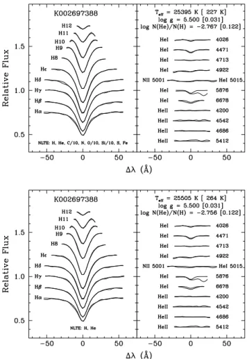
Among others, a 3D grid of 1440 NLTE model atmospheres and synthetic spectra was constructed for this specific metallic-ity. The grid consists of 16 grid points in Teff spanning a range of 20 000−50 000 K in steps of 2000 K, 10 values of log g cov-ering the range 4.6−6.4 in steps of 0.2 dex, and 9 values of log N(He)/N(H) spanning the range of −4.0 to 0.0 in steps of 0.5 dex. For comparison purposes (see below), two other similar grids were also used, one with NLTE models but no metals, and the other one based on the LTE approximation and no metals. For each grid, we fitted our observed spectrum in 3D space, with the help of a χ2minimization technique first developed by Pierre Bergeron (see Saffer et al. 1994, for details). The upper panel of Fig.1shows the best fit we obtained for KIC02697388, lead-ing to Teff= 25 395 ± 227 K, log g = 5.500 ± 0.031 (cgs), and log N(He)/N(H) = −2.767 ± 0.122. We point out that the quoted uncertainties are formal errors in the fits and do not include systematic effects that remain difficult to evaluate. To provide a measure of the effects of metals, we also fitted our spectrum using equivalent NLTE models, but without metals (lower panel of Fig.1). The values now come out as Teff = 25 505± 264 K, log g = 5.500 ± 0.031 (cgs), and log N(He)/N(H) = −2.757 ± 0.122, indicating that the presence of metals (at least with the amounts assumed) is not a critical issue in the determination of the atmospheric parameters of KIC02697388. The map shown in Fig. 1 ofBrassard et al.(2010) indicates that, at the values of Teffand log g inferred for that star, the effects of metal blan-keting are indeed quite small in sdB atmospheres. Likewise, we find that NLTE versus LTE models lead to similar results; in the latter case, using our grid of LTE models with no metals, we find that Teff = 25 688± 276 K, log g = 5.517 ± 0.031 (cgs), and log N(He)/N(H) = −2.719 ± 0.118. We do not know why our estimates of the atmospheric parameters of KIC02697388 differ significantly from those given inØstensen et al.(2010).
Figure2shows a sample of short period (in blue) and long period (in red) sdB pulsators whose surface parameters have been derived using the same telescope/instrument combination, reduction procedure, and grid of model atmospheres, thereby
Fig. 1. Upper panel: model fit (heavy curve) to all the hydrogen and strong helium lines (thin curve) available in our high S/N, low-resolution optical spectrum of KIC 02697388. The fit was done using a 3D grid of NLTE synthetic spectra (Teff , log g, log N(He)/N(H)) in which the abundances of C, N, O, S, Si, and Fe were held fixed at amounts consistent withBlanchette et al.(2008). Lower panel: similar, but for a 3D grid of NLTE synthetic spectra without metals.
forming a homogeneous set. This homogeneity is a valuable property that ensures the position of each star relative to the others in the log g−Teff plane should be correct, even though systematics of unknown nature may affect the determination of their parameters on an absolute scale. The atmospheric param-eters derived for KIC02697388 (represented as a green square with a cross in the figure) place the star among the coolest pul-sating hot B subdwarfs. Its position in the diagram is consistent with the presence of long period oscillations.
2.2. Kepler time series photometry
The hot B subdwarf star KIC02697388 was observed by Kepler in short cadence mode (58.8 s sampling rate) over a time base-line of ∼27.11 days (∼650.73 h) from August 20 to September 16, 2009 (run Q2.3; seeØstensen et al. 2010). The data were pro-cessed through the Kepler Science Processing Pipeline (Jenkins et al. 2010). A preliminary analysis of the light curve obtained for this star was presented inReed et al.(2010) as part of a gen-eral report on the frequencies observed in sevgen-eral long period sdB pulsators discovered during the first part of the Kepler ex-ploratory program (Q0, Q1, and Q2 runs). To exploit these data
Fig. 2.Distribution of the hot B subdwarf pulsators in the log g−Teff plane from a sample of 28 short-period (out of 51 known; in blue) and 33 long-period (out of 45 known; in red) sdB pulsators. Three stars in this sample show both long- and short-period pulsations (blue filled circles within a red annulus). We stress that the plotted stars form a ho-mogeneous sample in terms of the determination of their atmospheric parameters (based on our NLTE metal-free H/He model atmospheres). On the same homogeneous scale, the green square with a cross marks the position of KIC02697388. The overplotted blue contours indicate the number of driven $ = 0 p-modes (the largest contour corresponds to one driven mode) and manifest the p-mode instability region derived from models assuming iron distributions at equilibrium between gravi-tational settling and radiative levitation (Charpinet et al. 2001). Nearly all p-mode pulsators are concentrated within the three highest contours (solid lines) where driving is most efficient.
for a detailed asteroseismic study of KIC02697388, we need a more thorough frequency analysis that we provide here.
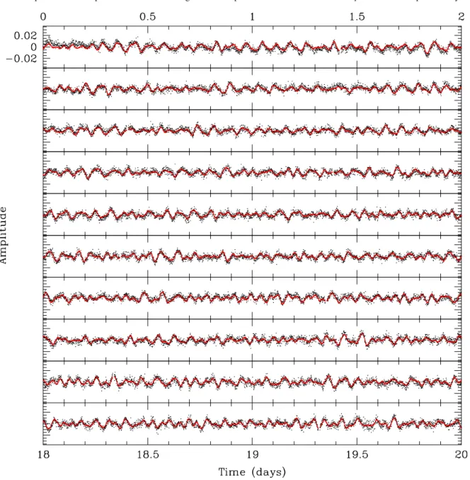
Figure3shows a 20-day-long section of the Kepler “white light” photometry of KIC02697388. We based the following analysis on the raw light curve. The choice of using raw data instead of data preliminary corrected for contamination has no impact on the seismic analysis. The only significant difference appears in the measured amplitudes of the modulations, which, for this star, are found to be larger by ∼20% for the corrected data. To maximize the signal-to-noise ratio of the data in Fourier space, the light curve was detrended for residual long-term vari-ations and cleaned of data points that differ significantly from the local standard deviation by applying a running 3-σ clipping filter. After this treatment, an effective duty cycle of ∼96% is reached, resulting in a window function so pure that aliasing due to interruptions never interfere with the identification of real fre-quencies. In this light curve, low-amplitude multi-periodic os-cillations with dominant periodicities around 1–2 h are clearly seen. The complex interference pattern indicates that a signif-icant number of modes are involved in the brightness modula-tion, as outlined byReed et al.(2010), who conclude that at least 37 frequencies must be present.
A Lomb-Scargle periodogram (LSP;Scargle 1982) of the light curve confirms the complex multi-periodic nature of the
star brightness modulation. The region where dominant signal is clearly detected covers the range 60–400 µHz (left panel of Fig.4). The timescale of these modulations (∼1–4 h) is typical of the variations induced by g-mode pulsations in long period sdB pulsators. Another frequency region also shows modula-tions with weak but significant signal in the 500–1100 µHz range (right panel of Fig.4). More surprisingly, as noted byReed et al. (2010), we also find a very weak periodic signature at a much shorter timescale (see Fig.5), which, if real, is quite unexpected, at first sight, for a cool sdB star such as KIC02697388. This fre-quency would indeed be comparable to variations generally en-countered in the short period p-mode sdB pulsators, which are found at higher effective temperatures. We provide evidence that this short period modulation is indeed very likely to be caused by an excited acoustic mode, making KIC02697388 a hybrid sdB pulsator (see Sect. 3.4). All other frequency regions, not illus-trated here, up to the Nyquist limit (∼8500 µHz) are otherwise found to be consistent with noise.
We applied the usual prewhitening and nonlinear least squares fitting techniques to extract the frequencies (Deeming 1975). We used a dedicated software program, FELIX (Frequency Extraction for LIghtcurve eXploitation) developed by one of us (S.C.), which greatly eases and accelerates the ap-plication of this procedure, especially for long time series ob-tained from space (Charpinet et al. 2010). The procedure was performed with no major difficulty, thanks to the very high qual-ity of the Kepler photometry. However, on several occasions, groups of seemingly unresolved peaks were encountered, as al-ready mentioned inReed et al.(2010). Dealing with close peaks that differ by less than ∼1.5 times the formal resolution of the data (which is ∼0.43 µHz in the present case) can be prob-lematic. In several instances, the simultaneous nonlinear least squares fitting method could not converge for the close frequen-cies. Our approach in these cases was to first select the dominant frequency of a crowded complex, perform the simultaneous non-linear least squares fit on the frequency, amplitude, and phase, and freeze the frequency to the value obtained (keeping ampli-tude and phase as free parameters). Other close peaks of lower amplitude associated with that complex could then be selected, fitted individually for frequency, amplitude, and phase and then fitted simultaneously with the other peaks while keeping their frequency locked. This procedure allowed us to extract all the peaks in the Fourier domain beyond a given detection thresh-old where we used, as usual, 4σ above the mean noise level. Nonetheless, one must keep in mind that the uncertainties asso-ciated with the frequencies derived for the unresolved peaks are, in fact, somewhat larger (around the formal resolution of the run, to be conservative) and that, except for the main peak of a com-plex that is certainly real, the existence of some of the lower am-plitude components may be questionable. We stress however that these uncertainties only marginally affect our subsequent seismic analysis (see the next section).
Table1lists the 63 peaks that we extracted from the Kepler light curve. The table also provides their attributes: frequency, period, amplitude, and phase (with their error estimates σf, σP,
σA, and σPh, respectively), as well as the signal-to-noise ratio of the detection. Among the 63 frequencies, four (labeled “an”) are
known as instrumental artifacts1 and 59 (labeled “ f
n”, where n
1 a1, a
2, and a4 are harmonics of an electronic crosstalk with the long cadence readout operation that occurs with a frequency fLC = 566.391 µHz. a3is likely another artifact of unclear origin since it is observed in the light curves of several other stars (seeØstensen et al. 2010).
Fig. 3.Twenty day section of the light curve obtained for KIC02697388 during Q2.3 Kepler observations. The amplitude as a function of time is expressed in terms of the residual relative to the mean brightness intensity of the star. The red curve shows the reconstructed signal based on the extracted frequencies, amplitudes, and phases given in Table 1.
is ranked in order of the decreasing amplitude of the main peak) are presumably pulsation modes. In this table, close unresolved frequencies separated by less than ∼1.5 times the formal reso-lution (i.e., ∼0.65 µHz) are grouped together. We also note that the phase is relative to the beginning of the run. This zero point corresponds, in the solar system barycentric reference frame, to BJD 2 455 064.3628260 (time standard is UTC) and the fitted waves have the form A cos[2π/P(t − phase)]. The noise level is extremely low, ranging from ∼0.0054% (54 ppm) at low fre-quencies to ∼0.0027% (27 ppm) at high frefre-quencies. The recon-structed light curve based on all the harmonic oscillations given in Table1is shown in Fig.3plotted (in red) over the observed light curve. In a similar way, Fig.4 shows the Lomb-Scargle periodogram of the observed time series in relevant frequency regions and, plotted upside-down, its reconstruction based on all frequencies from Table1. The LSP of the residual light curve after subtracting all oscillations is also given, shifted downward. In both the time domain (Fig.3) and frequency space (Fig.4),
the reconstruction based on the fitted modulations closely repro-duces the observations.
The comparison of our Table1with Table 3 ofReed et al. (2010) finds excellent agreement. In our present analysis, how-ever, 22 additional frequencies (listed within brackets in Table1) are not reported inReed et al.(2010). The reasons are twofold: 1) we used a different estimate of the detection threshold, the one adopted byReed et al.(2010) being slightly more conservative, and 2) in their preliminary analysis,Reed et al.(2010) did not extract all the apparent peaks in the poorly resolved groups of close frequencies.
3. Seismic analysis 3.1. Method and models
For the seismic analysis, we adopt a variant of the forward-modelling approach applied with success to the study of several
Fig. 4.Lomb-Scargle periodogram (LSP) in the 50–450 µHz frequency range (left panel) and the 450–1100 µHz frequency range (right panel), where signal is found. The reconstructed LSP based on the extracted harmonic oscillations given in Table1(indicated by red vertical segments) is shown upside down. The curve shifted downward is the LSP of the residual (i.e., noise) after subtracting all the frequencies of Table1from the observed light curve.
Fig. 5.Lomb-Scargle periodogram (LSP) in the 3785–3830 µHz fre-quency range where a weak signal is also suspected. The green (blue, red) dotted curves refer to a value equal to 4.0 (3.6, 3.0) times the local mean noise level. The indicated peak at 3805.94 µHz ( f38in Table1) clearly emerges at 5.7 times the average noise.
p- and g-mode sdB pulsators. The method was described in de-tail inCharpinet et al.(2005,2008) and relies on fitting simulta-neously all of the observed pulsation frequencies with theoretical frequencies calculated for appropriate hot B subdwarf models. The quality of the fit is quantified using a merit function defined as S2(p1, ...,pn) = Nobs ! i=1 (νobs,i− νth,i)2, (1)
where Nobs is the number of observed frequencies and {νobs,i, νth,i} are the associated pairs of observed/computed fre-quencies. This quantity, S2, needs to be minimized as both a function of the frequency associations (i.e., a combinatorial first minimization required because the observed modes are not identified a priori) and as a function of the model parame-ters, {p1, ...,pn}. For that purpose, we developed efficient
op-timization codes to find the minima of the merit function (a
multi-dimensional function that can be of very complex shape), which constitute the potential asteroseismic solutions. Utilizing this procedure, we obtain the mode identification (i.e., the most closely fitting association between observed and theoretical fre-quencies) and, more importantly, constraints on the main struc-tural parameters of the star.
Quantitative asteroseismology of g-mode pulsators has be-come possible thanks to our so-called “third-generation” (3G) models, which is suitable for the accurate evaluation of g-mode pulsation frequencies. These 3G models are briefly described in Brassard & Fontaine(2008, 2009). They are complete stellar structures in thermal equilibrium defined in terms of a set of pa-rameters inspired from full evolutionary models. The reason we use static parametrized structures instead of evolutionary models is that the former provide the needed flexibility for thoroughly exploring parameter space. The input parameters needed to char-acterize a 3G model are: the total stellar mass M∗, the frac-tional mass of the outer hydrogen-rich envelope log(Menv/M∗), the fractional mass of the mixed convective core log(Mcore/M∗), and the chemical composition of the core (with the constraint X(He) + X(C) + X(O) = 1). The effective temperature, Teff, and surface gravity, log g, are computed a posteriori for a 3G model of given parameters. To exploit the atmospheric parameters de-termined independently by spectroscopy, we incorporate the val-ues of Teffand log g as external constraints in the optimization procedure to search for a best-fit model. Only the models de-fined by minima in the S2merit function that have atmospheric parameter values within a given tolerance around the spectro-scopic estimates are considered acceptable, thus ensuring, by construction, consistency with spectroscopy. In the specific case of KIC02697388, acceptable solutions have to fall in the ranges of 3σ around Teff = 25 395 K and log g = 5.500. We note that there is no guarantee, a priori, that a good frequency match exists within these constraints.
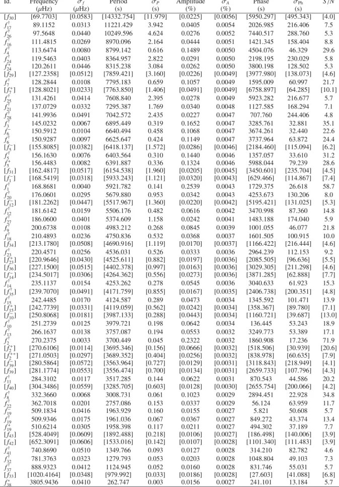
Table 1. List of frequencies, fn, and known instrumental artefacts, an, detected four times above the noise level.
Id. Frequency σf Period σP Amplitude σA Phase σPh S/N
(µHz) (µHz) (s) (s) (%) (%) (s) (s) [ f30] [69.7703] [0.0583] [14332.754] [11.979] [0.0225] [0.0056] [5950.297] [495.343] [4.0] f† 17 89.1152 0.0313 11221.429 3.942 0.0405 0.0054 2026.985 216.406 7.5 f26† 97.5648 0.0440 10249.596 4.624 0.0276 0.0052 7440.517 288.760 5.3 f† 16 111.4815 0.0269 8970.096 2.164 0.0444 0.0051 1421.345 158.404 8.8 f† 4 113.6474 0.0080 8799.142 0.616 0.1489 0.0050 4504.076 46.329 29.6 f† 24 119.5463 0.0403 8364.957 2.822 0.0291 0.0050 2198.195 230.029 5.8 f+ 24 120.2611 0.0446 8315.238 3.084 0.0262 0.0050 3800.198 128.502 5.3 [ f29] [127.2358] [0.0512] [7859.421] [3.160] [0.0226] [0.0049] [3977.980] [138.073] [4.6] f† 7 128.2844 0.0108 7795.183 0.659 0.1057 0.0049 1595.009 60.997 21.7 [ f+ 7] [128.8021] [0.0233] [7763.850] [1.406] [0.0491] [0.0049] [6758.897] [64.285] [10.1] f† 25 131.4261 0.0414 7608.840 2.395 0.0278 0.0049 5923.282 216.677 5.7 f† 21 137.0729 0.0332 7295.387 1.769 0.0340 0.0048 1127.585 168.294 7.1 f28† 141.9936 0.0491 7042.572 2.435 0.0227 0.0047 707.760 244.406 4.8 f† 3 145.0232 0.0067 6895.449 0.319 0.1652 0.0047 3285.761 32.881 35.1 f− 6 150.5912 0.0104 6640.494 0.458 0.1068 0.0047 3674.261 32.440 22.6 f† 6 150.9287 0.0097 6625.647 0.424 0.1149 0.0047 3737.964 63.872 24.4 [ f− 5] [155.8085] [0.0382] [6418.137] [1.572] [0.0286] [0.0046] [2184.460] [115.094] [6.2] f† 5 156.1630 0.0076 6403.564 0.310 0.1440 0.0046 1357.057 33.610 31.2 f+ 5 156.4483 0.0082 6391.887 0.336 0.1324 0.0046 5988.044 79.239 28.6 [ f31] [162.4817] [0.0517] [6154.538] [1.960] [0.0205] [0.0045] [3450.601] [235.704] [4.5] [ f− 1] [168.5419] [0.0318] [5933.243] [1.121] [0.0320] [0.0043] [629.466] [114.867] [7.4] f† 1 168.8681 0.0040 5921.782 0.141 0.2539 0.0043 1729.375 26.618 58.7 f† 20 176.0601 0.0295 5679.880 0.953 0.0342 0.0043 4253.673 130.206 8.0 [ f− 12] [181.2262] [0.0447] [5517.967] [1.360] [0.0220] [0.0042] [5195.421] [131.025] [5.3] f† 12 181.6142 0.0159 5506.176 0.482 0.0616 0.0042 3470.998 87.360 14.8 f† 27 186.0600 0.0401 5374.609 1.158 0.0242 0.0041 1483.188 174.040 5.9 f† 9 200.6738 0.0108 4983.212 0.268 0.0845 0.0039 1001.055 46.077 21.8 f† 18 210.4893 0.0236 4750.836 0.532 0.0368 0.0037 1601.505 100.915 10.0 [ f34] [213.1780] [0.0508] [4690.916] [1.119] [0.0170] [0.0037] [1166.422] [216.444] [4.6] f† 23 220.4571 0.0256 4536.031 0.526 0.0333 0.0036 2964.239 112.153 9.2 [ f+ 23] [220.9646] [0.0430] [4525.611] [0.882] [0.0197] [0.0036] [2085.505] [96.636] [5.5] [ f36] [227.1500] [0.0515] [4402.378] [0.997] [0.0163] [0.0036] [3029.305] [211.298] [4.6] [ f− 14] [234.5017] [0.0306] [4264.362] [0.556] [0.0273] [0.0036] [3871.285] [62.888] [7.7] f† 14 235.1137 0.0154 4253.262 0.278 0.0545 0.0036 3040.633 61.923 15.3 [ f† 35] [239.7070] [0.0491] [4171.759] [0.855] [0.0167] [0.0035] [2406.738] [200.351] [4.8] f† 15 242.4485 0.0170 4124.587 0.289 0.0473 0.0034 1345.592 101.471 13.9 [ f+ 15] [242.7739] [0.0331] [4119.059] [0.562] [0.0242] [0.0034] [358.367] [89.780] [7.1] [ f− 10] [250.8068] [0.0181] [3987.133] [0.288] [0.0443] [0.0034] [1160.721] [39.687] [13.0] f† 10 251.2739 0.0125 3979.721 0.198 0.0642 0.0034 136.445 53.243 18.9 f† 13 266.1637 0.0138 3757.087 0.194 0.0553 0.0032 3249.773 53.389 17.1 f† 2 270.2375 0.0033 3700.449 0.045 0.2322 0.0032 1860.908 17.236 71.9 [ f+ 2] [270.6106] [0.0114] [3695.346] [0.156] [0.0666] [0.0032] [518.506] [30.939] [20.6] [ f++ 2 ] [271.0503] [0.0297] [3689.352] [0.404] [0.0256] [0.0032] [838.978] [60.635] [7.9] [ f− 39] [280.5864] [0.0572] [3563.964] [0.727] [0.0129] [0.0031] [3118.843] [218.949] [4.1] [ f39] [281.1774] [0.0553] [3556.474] [0.700] [0.0134] [0.0031] [2659.733] [107.796] [4.3] f† 11 284.3102 0.0117 3517.285 0.144 0.0622 0.0031 870.543 44.586 20.2 [ f40] [304.3486] [0.0559] [3285.705] [0.603] [0.0128] [0.0030] [2655.754] [200.066] [4.2] f† 8 332.3660 0.0068 3008.731 0.061 0.1023 0.0029 2894.451 22.928 34.8 f† 22 362.7018 0.0201 2757.086 0.153 0.0337 0.0029 56.124 63.959 11.7 f− 19 509.1834 0.0416 1963.929 0.160 0.0155 0.0027 5.821 50.608 5.7 f† 19 509.9346 0.0175 1961.036 0.067 0.0367 0.0027 849.272 43.374 13.4 f+ 19 510.6214 0.0305 1958.398 0.117 0.0211 0.0027 494.302 37.189 7.7 [ f43] [528.4049] [0.0609] [1892.488] [0.218] [0.0106] [0.0027] [186.498] [140.006] [3.9] [ f42] [652.3091] [0.0606] [1533.016] [0.142] [0.0107] [0.0028] [1101.340] [111.483] [3.9] f† 41 740.8690 0.0510 1349.766 0.093 0.0127 0.0028 314.210 82.782 4.6 f† 32 781.3763 0.0323 1279.793 0.053 0.0203 0.0028 1048.804 49.103 7.3 f† 37 888.9323 0.0412 1124.945 0.052 0.0160 0.0028 831.746 55.031 5.7 [ f33] [1020.4164] [0.0348] [979.992] [0.033] [0.0186] [0.0028] [27.603] [41.088] [6.8] f∗ 38 3805.9436 0.0410 262.747 0.003 0.0156 0.0027 241.101 13.184 5.7
Table 1. continued.
Id. Frequency σf Period σP Amplitude σA Phase σPh S/N
(µHz) (µHz) (s) (s) (%) (%) (s) (s) Instrumental artefacts a2: 8 flc 4531.5510 0.0312 220.675 0.002 0.0192 0.0025 169.943 8.978 7.5 a1: 9 flc 5097.9751 0.0283 196.156 0.001 0.0227 0.0027 36.818 6.745 8.3 a3 7865.6389 0.0332 127.135 0.001 0.0186 0.0026 31.948 5.349 7.1 a4: 15 flc 8496.7276 0.0471 117.692 0.001 0.0138 0.0028 87.565 6.862 5.0
Notes. Frequency not reported in Reed et al. (2010);†frequency selected for the first step in the search of an asteroseismic solution;∗suspected p-mode.
3.2. Search for an optimal model
In the present seismic analysis of KIC 02697388, we adopt the following approach: first, to be conservative, we only consider a subset of frequencies (those marked with a “†” sign) that have been reported both in Table 1 and in Table 3 of Reed et al. (2010). In this way, the additional frequencies that we report do not interfere with the search of an optimal model, should some of these frequencies be spurious. A comparison can however be done afterward with the theoretical frequency spectrum of the se-lected solution. In a second step, we use all the independent fre-quencies (all the “ fn” listed in Table1) in the analysis. For each
group of close frequencies, we retain only the dominant com-ponent (in amplitude) as an independent pulsation mode. Other close frequencies are just ignored. The unresolved frequencies can be interpreted in various ways. A possibility is that the star is rotating slowly and the non-radial pulsation modes are split because of this rotation. Another option is that the amplitude and/or phase of some modes are not constant during the run and cannot be correctly prewhitened with waves that are assumed to be purely sinusoidal. We will be unable to decide whether this is possible until longer time series on this star (which Kepler will eventually provide) become available in order to resolve properly these fine structures in the amplitude spectrum. We emphasize, however, that the uncertainties associated with these unresolved features do not have a strong impact on the seismic analysis presented here.
For the first conservative approach, this leaves us with 32 frequencies that are assumed independent, while we end up with 43 independent frequencies when considering the entire spec-trum listed in Table1. In both cases, we attempt to match these frequencies simultaneously to modes computed from perfectly spherical (i.e, nonrotating) models. With this hypothesis, all quencies are considered as m = 0 modes and the theoretical fre-quency spectrum is defined only in terms of the k (radial order) and $ (degree) of the modes. We point out that, for slow rotators, the eventual error in misidentifying the m index of an observed frequency has a limited impact on the results of a seismic anal-ysis. This is true as long as the error induced on the frequency remains smaller than the overall accuracy achieved for the seis-mic fit, which will be the case for KIC02697388.
The search for best-fit solutions was carried out in the following domain: M∗/M$ ∈ [0.30, 0.70], log q(H) = log(Menv/M∗) ∈ [−5.0, −1.8], log qcore = log(1− Mcore/M∗) ∈ [−0.40, −0.10], and Xcore(C + O) ∈ [0.00, 0.99], where Xcore(C+O) is the fractional part (in mass) of carbon and oxy-gen in the core. The ranges considered for log q(H) and M∗rely on expectations from various formation scenarios for hot sub-dwarfs (Han et al. 2002,2003), whereas the limits on the core size are loosely inspired by horizontal branch stellar evolution-ary calculations (Dorman et al. 1993).
To restrict the search domain, we have to make additional assumptions about the nature of the modes that have been de-tected. Since the star was monitored photometrically, we usu-ally consider from the expected visibility of the pulsation modes that only low degree modes can be effectively seen. We typically limit the search to modes of degree $ ≤ 2, unless we are forced to consider higher $-values. Our first calculations assuming that the modes were only $ = 1 and 2 led us to realize that the light curve of KIC02697388 cannot be understood in terms of $ ≤ 2 modes only. Within this strict limitation on $, we were unable to find a suitable simultaneous fit to the observed frequencies and we concluded that some of the modes should be of higher $. In terms of visibility, beyond $ = 1 and 2, we expect to see prefer-entially the $ = 4 modes that, in sdB stars, are significantly less affected than $ = 3 modes by the geometric cancellation effect (Randall et al. 2005).
A closer look at the structure of the pulsation spectrum illus-trated in Fig.4(see also Table1) can also be instructive. In terms of amplitude distribution, we note that most of the higher am-plitude frequencies are concentrated in the 100–200 µHz range. Between 200 and 380 µHz, the amplitudes of the modes gen-erally appear to be smaller, except for one frequency, f2 at 270.24 µHz, which is the second highest peak. The range 380– 500 µHz forms a gap where no pulsation is detected and, again, peaks are found in the 500–1050 µHz domain, but all of them have an extremely small amplitude (the amplitude scale in the right panel of Fig.4is considerably wider than the left panel). Interestingly, this observed amplitude distribution can be linked with some theoretical expectations.Fontaine et al.(2003) pro-vided an extensive study of the driving mechanism responsible for the g-mode instabilities in hot B subdwarfs. Apart from the well-known discrepancy between the locations of the observed and theoretical instability strips that can possibly be resolved with the inclusion of nickel, in addition to iron, as a signifi-cant source of opacity (Jeffery & Saio 2006a,b,2007;Charpinet et al. 2009a),Fontaine et al.(2003) show that the range of fre-quency (period) where the g-modes are driven depends on the degree $. In particular, Fig. 9 ofFontaine et al.(2003) clearly indicates that as $ increases, shorter periods (higher frequencies) are driven. This behavior occurs because the excitation mech-anism acting on these g-modes drives a range of radial orders rather than a range of periods (frequencies) and, in the asymp-totic regime, the periods of modes with the same k value scale approximately as [$($ + 1)]−0.5. It is therefore tempting to inter-pret the observed frequency spectrum of KIC02697388 as the superposition of 3 series of modes of roughly the same range of radial order k but with $ = 1, 2, and 4. Since each series would be shifted by a factor [$($ + 1)]0.5from lower ($ = 1) to higher frequencies ($ = 4), with possibly a gap for the missing (i.e., hardly detectable) $ = 3 modes, this scheme matches quite well, at least qualitatively, the observed structure of the pulsation
-2.10 -2.15 -2.20 -2.25 -2.30 -2.35 -2.40 -2.45 -2.50 0.41 0.42 0.43 0.44 0.45 0.46 0.47 0.48 0.49 0.50 2.00 1.90 1.80 1.70 1.60 1.50 1.40 1.30 1.20 1.10 1.00 0.90 0.80 0.70 0.60 0.50 0.40 0.30 0.20 0.10 0.00 0.90 0.80 0.70 0.60 0.50 0.40 0.30 0.20 0.10 0.00 -0.40 -0.35 -0.30 -0.25 -0.20 -0.15 -0.10 2.00 1.90 1.80 1.70 1.60 1.50 1.40 1.30 1.20 1.10 1.00 0.90 0.80 0.70 0.60 0.50 0.40 0.30 0.20 0.10 0.00
Fig. 6.Left panel: slice of the S2function (in logarithmic units) along the M
∗− log q(H) plane with the parameters log q(core) and Xcore(C + O) fixed to their optimal values obtained in the best-fit seismic model 1. Right panel: slice of the S2function (in log) along the log q(core)−X
core(C + O) plane with the parameters M∗and log q(H) fixed to their optimal values. White contours show regions where the frequency fits have S2values within, respectively, the 1σ, 2σ, and 3σ confidence levels relative to the best-fit solution.
spectrum. Keeping these considerations in mind, we therefore consider for our forward modelling exploration that frequencies lower than 120 µHz should be $ = 1 modes, those lower than 500 µHz should be either $ = 1 or $ = 2 pulsation modes, and above 500 µHz, we allowed the frequencies to be associated with modes of degree $ = 1, 2, or 4. Associations with $ = 4 modes were also permitted for five frequencies (namely, f40, f39, f35, f36, and f34) because of their very low apparent amplitudes. In summary, this approach allows the very low amplitude frequen-cies to be $ = 4 modes, while there is still a possibility that they are associated with modes of degree $ = 1 or 2, if these mode frequencies fit better.
Within the search domain specified, and taking into consid-eration the external constraints on atmospheric parameters, we first ran the optimization code on the reduced set of 32 frequen-cies (i.e., the conservative approach). This search revealed that two families of models provide the most accurate possible match to the considered frequencies. The main parameters of these two model solutions are summarized in Table2. Both solutions turn out to be essentially equal in terms of quality of fit (the value of S2/N
obs). The frequency match (not given here) shows that the two families differ slightly at the level of the mode identifica-tion, but do not provide additional arguments that would allow us to favor one of the solutions over the other. Looking at the 11 additional frequencies that were not considered in this first exploration, we realized that all of them can be associated with modes present in the theoretical pulsation spectrum of both fam-ilies of models, without their quality of fit being degraded sig-nificantly. This a posteriori match is highly unlikely to occur by chance and we interpret it as a clear indication that these addi-tional frequencies not reported inReed et al.(2010) are real. In this context, we re-ran the optimization code using the full set of 43 frequencies (i.e., including all the independent frequencies identified in our analysis presented in Sect. 2). This new search, as expected, also uncovered evidence of two families of solu-tions with only slightly differing parameters. These solusolu-tions are
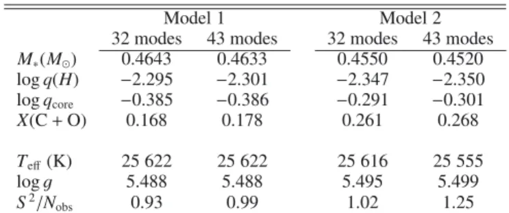
Table 2. The two families of solutions based on 32 modes or 43 modes.
Model 1 Model 2
32 modes 43 modes 32 modes 43 modes
M∗(M$) 0.4643 0.4633 0.4550 0.4520 log q(H) −2.295 −2.301 −2.347 −2.350 log qcore −0.385 −0.386 −0.291 −0.301 X(C + O) 0.168 0.178 0.261 0.268 Teff(K) 25 622 25 622 25 616 25 555 log g 5.488 5.488 5.495 5.499 S2/Nobs 0.93 0.99 1.02 1.25
also given in Table2. The models obtained by simultaneously fitting 32 modes or 43 modes clearly do not differ significantly. With 43 modes, model 1 may appear slightly better than model 2 in terms of quality of fit (S2/N
obsvalue), but the difference is in-significant and we objectively cannot, at this stage, select one of these models as the true solution. We emphasize that both solu-tions show excellent agreement with spectroscopic estimates of the effective temperature and surface gravity.
The maps shown in Figs.6and7illustrate the behavior of the merit function in the vicinity of each best-fit seismic solu-tion. In both panels, the merit function S2incorporates the spec-troscopic constraints on atmospheric parameters. To create these plots, we tolerated a deviation of 3σ for the effective tempera-ture and 2σ for the surface gravity. An exponential correction factor multiplies the merit function if the model effective tem-perature and surface gravity are outside these ranges, in effect degrading the S2value of the model. The panels clearly indicate deep blue regions (corresponding to best-fitting models, i.e., low values of S2) in the M
∗− log q(H) and log q(core)−Xcore(C + O) planes, which are well-defined by the pulsation spectrum and the spectroscopic constraints. The regions in red correspond to mod-els that are inconsistent with spectroscopic values within the tol-erance mentioned above or that provide a very poor match to the
-2.10 -2.15 -2.20 -2.25 -2.30 -2.35 -2.40 -2.45 -2.50 0.41 0.42 0.43 0.44 0.45 0.46 0.47 0.48 0.49 0.50 2.00 1.90 1.80 1.70 1.60 1.50 1.40 1.30 1.20 1.10 1.00 0.90 0.80 0.70 0.60 0.50 0.40 0.30 0.20 0.10 0.00 0.90 0.80 0.70 0.60 0.50 0.40 0.30 0.20 0.10 0.00 -0.40 -0.35 -0.30 -0.25 -0.20 -0.15 -0.10 2.00 1.90 1.80 1.70 1.60 1.50 1.40 1.30 1.20 1.10 1.00 0.90 0.80 0.70 0.60 0.50 0.40 0.30 0.20 0.10 0.00
Fig. 7.Same as Fig.6but for model solution 2.
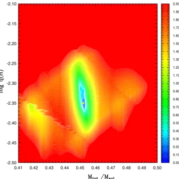
observed frequencies. The two uncovered valleys clearly show solutions that are significantly better in reproducing the observed pulsation spectrum than any other surrounding area of the pa-rameter space. To verify whether the two solutions are truly dis-tinct, we calculated a large 4-dimensional grid of 333 268 mod-els focusing on the region, in parameter space, that contains the two identified models. Figure8 shows a map representing the “projection” (S2, in logarithmic scale) of the 4D S2 function constructed from this grid on the log q(core)−Xcore(C + O) plane. This projection is defined as
S2(p
1,p2) = min{S2(p1,p2,p2,p3); ∀p2,∀p3}, (2) where p1 = log q(core), p2 = Xcore(C + O), p3 = M∗, and p4 = log q(H). In other words, since we are interested in the minima of the merit function (the best-fit models), at each lo-cus of the represented plane, the value given (S2) is the lowest value of S2 among those found for all M
∗ and log q(H) varied independently. This map illustrates that the two families of solu-tions are indeed unconnected valleys. The two regions of best-fit models (dark blue areas) remain confined to quite narrow ranges for the log q(core) parameter, but show some elongation in the Xcore(C + O) direction. The domain confined within the 1σ con-tours provides, for each solution, a conservative estimate of the internal precision at which these parameters are effectively mea-sured for KIC02697388.
Similarly, Fig.9shows the “projection” of S2, but this time onto the M∗− log q(H) plane. The represented quantity is now S2(p
2,p3) = min{S2(p1,p2,p2,p3); ∀p1,∀p2}, (3) where the {pj}’s are defined as before, i.e., at each locus of
the represented plane, the value given (S2) is the lowest value of S2 among those found for all log q(core) and X
core(C + O) varied independently. The two solutions clearly overlap in the M∗− log q(H) plane, forming a joint area. The domain confined within the 1σ contours provides a conservative estimate of the internal precision at which M∗and log q(H) are effectively mea-sured for KIC02697388 (see Sect. 3.5).
0.34 0.32 0.30 0.28 0.26 0.24 0.22 0.20 0.18 0.16 0.14 0.12 0.10 -0.40 -0.38 -0.36 -0.34 -0.32 -0.30 -0.28 -0.26 2.00 1.90 1.80 1.70 1.60 1.50 1.40 1.30 1.20 1.10 1.00 0.90 0.80 0.70 0.60 0.50 0.40 0.30 0.20 0.10 0.00
Fig. 8.Expanded view of the log q(core)−Xcore(C + O) region where the two model solutions are found. The map represents S2, a “projection” of the 4-dimensional S2 function (in log scale): at each log q(core), Xcore(C + O) position, the value given is the minimum of log S2that can be found among the values obtained for all M∗and log q(H). White con-tours show regions where the frequency matches have S2values within, respectively, the 1σ , 2σ , and 3σ confidence levels relative to the best-fit solution. The yellow marks indicate the positions of the two solutions found by the optimization code.
3.3. Frequency match and mode identification
The two model solutions isolated for KIC02697388 provide very good simultaneous matches to the 43 observed frequencies (but see below). Details of both the fit and mode identification are
-2.20 -2.25 -2.30 -2.35 -2.40 -2.45 0.440 0.445 0.450 0.455 0.460 0.465 0.470 0.475 0.480 2.00 1.90 1.80 1.70 1.60 1.50 1.40 1.30 1.20 1.10 1.00 0.90 0.80 0.70 0.60 0.50 0.40 0.30 0.20 0.10 0.00
Fig. 9.Same as Fig.8but the projection is done onto the M∗− log q(H) plane.
given, for both models, in Tables3and4, respectively (these ta-bles are provided as online material only). Figure10also pro-vides a graphical illustration of the fits. These tables list the most relevant computed frequencies νth(periods; Pth) with some useful properties (such as the kinetic energy, log Ekin, and the Ledoux coefficient, Ck$, associated with the mode; see, e.g.,
Charpinet et al. 2000) and show their association with the ob-served frequencies. For each pair of associated frequencies, the quantities ∆P = Pobs− Pth, ∆ν = νobs− νth, and ∆P/P = −∆ν/ν quantify the difference between the computed and measured val-ues. For convenience, we also provide again, in these tables, the amplitude of the observed mode. Finally, we indicate within brackets the 11 additional frequencies that were not reported in Reed et al.(2010).
For model 1, the averaged relative dispersion is |∆X/X| ∼ 0.35% (X = P or ν), which corresponds, on an absolute scale, to |∆P| = 20.9 s and |∆ν| = 0.811Ãl’µHz. The standard deviations in these quantities are, respectively, 24.8 s and 0.787 µHz. For model 2, the averaged relative dispersion is |∆X/X| ∼ 0.39%, corresponding to |∆P| = 23.0 s and |∆ν| = 0.957 µHz. The stan-dard deviations are then, respectively, 24.2 s and 0.918 µHz. Compared to previous analyses of g-mode sdB pulsators that were able to reproduce the frequencies with an average relative dispersion of ∼0.23% (seeVan Grootel et al. 2010a,b), we find that the quality of the frequency fits achieved for KIC 02697388 shows a noticeable degradation. The larger number of modes that must be fitted simultaneously could possibly be one of the rea-sons why our best solutions for KIC02697388 do not as closely reproduce the observed spectrum as in the two other stars anal-ysed thus far. However, it is also likely that our current inability to resolve properly all the pulsation modes contributes signifi-cantly to the larger dispersion between the best-fit models and the observations. The induced uncertainties in the accuracy of some of the frequencies used in this analysis and possible mis-identifications of which component of a complex of modes is the m = 0 mode (if rotation plays a role) could indeed interfere at a level close to the formal frequency resolution of the present data
(∼0.43 µHz). Future time series obtained for this star with Kepler will undoubtedly improve the situation but, for the time being, this source of uncertainty remains sufficiently small to allow us to engage the detailed asteroseismic study of this star.
The 43 pulsations involved in our analysis are identified as low-degree ($ = 1, 2, and 4), intermediate-order (k = −7 through −64) g-modes2. We point out that almost all the very low
am-plitude frequencies above 500 µHz that were allowed to be ei-ther $ = 1, 2, or 4 modes, turn out to be identified as $ = 4 modes. This confirms our initial intuition that these low ampli-tude frequencies could indeed be the dominant modes belonging to the $ = 4 series that, despite strong geometrical cancellation (see Fig.11 and comments below), can emerge above the de-tection threshold of the present data (see Sect. 3.1). Looking at the amplitude distribution resulting from the mode identifi-cations derived from each solution, we clearly find that, in both cases, the highest amplitude frequencies are preferentially asso-ciated with $ = 1 modes, as one would expect. To quantify this, we point out that, for model 1 (Table3), eight frequencies were associated with $ = 4 modes. The average amplitude of these eight modes is A4,8m = 0.0186%. In comparison, we computed the average amplitudes, A1,8m and A2,8m, of the eight strongest modes associated with $ = 1 and $ = 2, respectively. We find that A1,8m= 0.1316 % and A2,8m= 0.0787 %. We therefore ob-tain the following average amplitude ratios of different degrees: A1,8m/A2,8m) 1.7, A1,8m/A4,8m) 7.1, and A2,8m/A4,8m) 4.2. For model 2 (Table4), the amplitude distribution is similar and we have A4,7m = 0.0188% (with only seven modes associated with $ = 4 in this case), A1,7m = 0.1362%, and A2,7m = 0.0983%. The corresponding average amplitude ratios of different degrees become A1,7m/A2,7m) 1.4, A1,7m/A4,7m) 7.2, and A2,7m/A4,7m) 5.2. In both cases, the pronounced amplitude separation between $ = 1, 2 and $ = 4 is qualitatively in line with the visibilities gen-erally expected from computations (see, Fig.11).
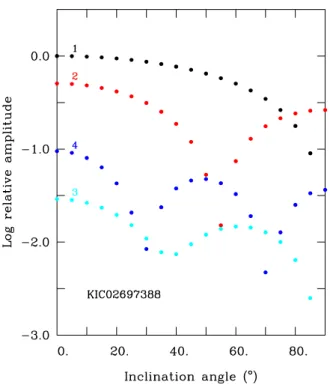
A more quantitative comparison of the averaged observed amplitude ratios with calculations remains however difficult for several reasons. Figure11shows the visibilities of $ = 1, 2, 3, and 4 modes expected for a star with parameters representative of KIC02697388. For g-modes in sdB stars, the light modula-tions are completely dominated by the temperature perturbation. These visibility curves were computed assuming the same intrin-sic amplitude for the temperature perturbation and only m = 0 modes were considered. The results are found to be indepen-dent of the pulsation frequency. The relative visibility of a mode clearly depends quite strongly on the (unknown) inclination an-gle of the star relative to the observer. The $ = 3 modes are the most affected by the geometrical cancellation effects except at very specific inclinations (i ∼ 30◦ and i ∼ 70◦). There is a marked gap between $ = 3, 4 and $ = 1 and 2 at nearly all viewing angles (except for i ∼ 55◦ and i ∼ 90◦). In the seismic analysis of KIC02697388, we assumed that all the observed fre-quencies were m = 0 modes (as in Fig.11), considering that, in the context of a star likely rotating relatively slowly, misidenti-fications of the m-index of the modes do not have a large im-pact on the asteroseismic solutions themselves. The visibility of the modes would however be greatly affected, depending on the inclination angle. An even more acute difficulty defeating meaningful quantitative comparisons of amplitude ratios is that the observed pulsation modes certainly do not have the same 2 We use, as a convenient convention, negative values for the radial order k of g-modes, while p-modes are identified with positive values of k.
Fig. 10.Distribution of the observed periods of KIC02697388 (in red) compared to the $ = 1, $ = 2, and $ = 4 g-mode theoretical pulsation spectrum of the optimal models 1 (left panel) and 2 (right panel). The radial order k of the computed modes is indicated for each series of degree.
Fig. 11.Relative amplitude (in logarithmic scale) of g-mode oscillations as a function of the inclination angle and the degree $ (assuming that m = 0). The values $ = 1 (black), 2 (red), 3 (cyan), and 4 (blue) are represented. These visibility functions are evaluated for a star with pa-rameters representative of KIC02697388 and in the Kepler band-pass.
intrinsic amplitudes. It is therefore very difficult, in these con-ditions, to go beyond the qualitative argumentation provided so far.
3.4. The high frequency oscillation
An intriguing feature of KIC02697388 revealed by the analysis of the Kepler light curve is the presence of a very weak, isolated peak at 3805.94 µHz (262.75 s; f38 in Table1). Our detailed asteroseismic study presented in the previous section demon-strate that this frequency is perfectly integrated into the best-fit solutions that emerge from this analysis and that it matches a low-order (k = 1) either radial ($ = 0) or non-radial ($ = 2) p-mode. These are the modes typically observed in sdBVrstars. A modulation at this short timescale, typical of the much hotter p-mode sdB pulsators, first raised skepticism regarding its true nature (real mode or instrumental artifact?). KIC02697388, ac-cording to our spectroscopy, is indeed one of the coolest known pulsating sdB stars and certainly among the last objects where we would expect to find acoustic modes. These modes are how-ever extremely sensitive to the surface gravity (log g) of the star and the remarkable correspondence with the best-fit solutions uncovered provides strong evidence of a real p-mode.
There is more, however, which brings us to Fig.2, where, as already mentioned, the position of KIC02697388 (green square with a cross) appears clearly separated from the other sdBVrand hybrid pulsators by more than 4 000 K. This figure also shows that there is no real conflict with theory on that surprising matter. The blue contours in Fig.2reproduce the expected instability re-gion for the short period p-mode pulsations derived from nonadi-abatic calculations (Charpinet et al. 2001). While all sdBVrand hybrid pulsators were, until now, always found within the three highest contours where the driving mechanism is most efficient to excite acoustic waves, the instability region actually covers a much larger region in the log g−Teff plane. The red edge, in particular, is found to reach significantly cooler effective tem-peratures, including most of the known long period g-mode pul-sators. KIC02697388, in particular, lies upon the edge of the in-stability region where models predict that one acoustic mode can
Table 5. Nonadiabatic properties of low-order, low degree p-modes in the optimal models.
Model solution 1 Model solution 2
Pobs Pth σI σ†I Pobs Pth σI σ†I $ k (s) (s) (s−1) (s−1) (s) (s) (s−1) (s−1) 0 2 ... 221.61 +3.819× 10⁻⁶ +2.642× 10⁻⁶ ... 215.83 +4.394× 10⁻⁶ +3.708× 10⁻⁶ 0 1 ... 269.50 −9.695 × 10⁻⁹ −1.583 × 10⁻⁷ 262.75 262.50 +1.303× 10⁻⁷ −6.588 × 10⁻⁹ 0 0 ... 331.83 −2.790 × 10⁻⁸ −2.902 × 10⁻⁸ ... 323.70 −2.320 × 10⁻⁸ −2.749 × 10⁻⁸ 1 3 ... 219.72 +4.277× 10⁻⁶ +3.122× 10⁻⁶ ... 214.08 +4.861× 10⁻⁶ +4.092× 10⁻⁶ 1 2 ... 267.47 +2.732× 10⁻⁸ −1.255 × 10⁻⁷ ... 260.63 +1.744× 10⁻⁷ +2.604× 10⁻⁸ 1 1 ... 327.27 −3.322 × 10⁻⁸ −2.228 × 10⁻⁸ ... 319.48 −2.696 × 10⁻⁸ −3.202 × 10⁻⁸ 2 2 ... 216.44 +5.043× 10⁻⁶ +3.851× 10⁻⁶ ... 211.21 +5.555× 10⁻⁶ +3.751× 10⁻⁶ 2 1 262.75 262.55 +1.350× 10⁻⁷ −1.254 × 10⁻⁸ ... 256.25 +2.900× 10⁻⁷ +8.184× 10⁻⁸ 2 0 ... 307.82 −2.112 × 10⁻⁸ −6.608 × 10⁻⁸ ... 294.61 −6.471 × 10⁻⁹ −4.148 × 10⁻⁸
Notes. † Value obtained when the amount of levitating Fe is increased by 8%.
still be excited. Looking into the details, we computed the nona-diabatic properties of the low-order low-degree p-modes in the two optimal solutions uncovered from the asteroseismic analy-sis. These can be found in Table5where, along with the com-puted period, Pth, we provide the nonadiabatic quantity σI (i.e.,
the imaginary part of the eigen-frequency) indicating if a mode is stable (σI > 0) or driven (σI < 0). Table5 shows that in
both cases, the mode associated with the observed periodicity is found to be stable but lies right next to the excited mode. Driving this mode would clearly require only a very slight modification of the models. For instance, increasing the effective temperature by only ∼100 K is sufficient to excite this mode. Alternatively, we find that a slight increase of only 8% in the amount of iron in the driving region (see, e.g., Charpinet et al. 2009b) is suffi-cient to make this mode unstable, as indicated in Table5. This result demonstrates that the presence of this high frequency is also consistent at the nonadiabatic level with the interpretation that it is a p-mode. The accumulation of evidence on this matter leads us to claim with confidence that the 262.75 s isolated sig-nal observed in KIC02697388 is a p-mode driven by the usual κ-mechanism and that this star is a hybrid pulsator.
The position of the red edge is a direct function of the amount of iron supported by radiative levitation in the stellar envelope. The contours reproduced in Fig.2are obtained by assuming that the iron abundance has reached a diffusive equilibrium state be-tween gravitational settling and radiative levitation. The distribu-tion of short period p-mode pulsators (including hybrids), prior to the discovery of KIC02697388, suggested that the true in-stability region was possibly much narrower than expected un-der this assumption. A natural explanation was that the equilib-rium abundance represents an upper limit that is not effectively reached because of competing processes. KIC02697388 some-what challenges this idea since an iron abundance at diffusive equilibrium, at least, is needed to account for the presence of this pulsation mode in this star. This object expands consider-ably the observed red edge of the p-mode pulsations in sdB stars. KIC02697388 also raises the question of the presence of very low amplitude p-modes in other long period sdB pulsators, most of them being significantly hotter and therefore more prone, in principle, to excite acoustic waves. The outcome of the Kepler survey phase reported inReed et al. (2010) and Baran et al. (2011) indeed provides indications that almost all other long pe-riod sdB pulsators may show such acoustic modes. The very low level of the amplitudes involved would naturally explains why these modes had never been detected before from the ground.
3.5. Derived stellar parameters
The asteroseismic analysis normally leads to the determination of the basic structural parameters of the scrutinized star. In the present situation, we do not have a single, clear-cut solution to propose for KIC02697388 but instead two solutions between which it is not possible to decide at this stage. We therefore de-rive two sets of parameters that reproduce equally well this star in terms of both spectroscopy and asteroseismology. These pa-rameters are summarized in Table6.
Estimating the 1σ (internal) uncertainties associated with the primary quantities (those naturally derived from the asteroseis-mic analysis) is an important, but nontrivial task. Adopting a conservative approach, we adapted the recipe described in detail inBrassard et al.(2001) andCharpinet et al.(2005), but instead of using the maps intersecting with the solutions (Figs.6and7), we considered the projected maps shown in Figs.8and9. The projection of the 1σ contour (i.e., the innermost white dashed contours shown in these figures) onto the various axis provides the 1σ estimate of the corresponding parameter. Because the so-lutions (the yellow marks) are generally not well centered in the region defined by the 1σ limit, the error estimates are given with differing plus and minus bounds. The uncertainties in the derived atmospheric parameters Teffand log g are obtained from the un-certainties in the primary quantities. To do so, we computed sev-eral models with parameters independently set to values corre-sponding to the various limits defining their 1σ range. The dif-ferences observed in Teffand log g with the corresponding values obtained for the optimal model were then added quadratically, thus providing an estimate of the global uncertainties in these quantities. A set of secondary parameters (stellar radius R, lumi-nosity L, age) is also derived on the basis of the primary parame-ters. Their associated errors are estimated in the same way as the uncertainties obtained for the effective temperature and surface gravity, i.e., by computing their values at the boundaries of the 1σ domain and adding the differences with the optimal model quadratically. To evaluate the age associated with each solution, we used new evolutionary models that incorporate the same in-put physics employed in our third generation static structures. These evolutionary calculations are described in a forthcoming paper (Brassard et al. 2011, in prep.). In particular, these mod-els include diffusion, gravitational settling, radiative levitation, core overshooting, and a time-dependent treatment for the con-vection. They also provide a treatment for the coupling between nuclear reactions and diffusion. To produce larger cores that can