Security management under uncertainty:
from day-ahead planning to intraday operation
P. Panciatici, Y. Hassaine, S. Fliscounakis, L. Platbrood, M. Ortega-Vazquez, J.L. Martinez-Ramos, L. Wehenkel
Abstract—In this paper, we propose to analyse the pratical
task of dealing with uncertainty for security management by Transmission System Operators in the context of day-ahead planning and intraday operation. We propose a general but very abstract formalization of this task in the form of a three-stage decision making problem under uncertainties in the min-max framework, where the three stages of decision making correspond respectively to operation planning, preventive control in operation, and post-contingency emergency control. We then consider algorithmic solutions for addressing this problem in the practical context of large scale power systems by proposing a bi-level linear programming formulation adapted to the case where security is constrained by power flow limits. This formulation is illustrated on two case studies corresponding respectively to a synthetic 7-bus system and the IEEE 30-bus system.
Index Terms—operation planning, intraday operation, security
management under uncertainties, transmission system operator, worst case analysis, mathematical programming
I. OUTLINE
D
AY-AHEAD operational planning as well as intraday operation of power systems is affected by an increasing amount of uncertainty due to the coupling of wind power intermittency, cross-border interchanges, market clearing, and load evolution. In this context, a deterministic approach that consists of forecasting a single best-guess of the system injections for the next day or hours, and of ensuring system security along this trajectory only, becomes inappropriate. The Transmission System Operator (TSO) will rather determine his strategic decisions by considering a set of scenarios reflecting his uncertainty and by making sure that under the worst of these scenarios the system security is still controllable.In this paper, we analyze the practical problem of security management in operation planning and intraday operation of large scale systems, and then formalize it in an abstract and generic way as a multi-stage decision making problem under uncertainties. We also propose and illustrate some practically feasible algorithms to address this problem for large scale systems. These algorithms are targeted towards solving a set of manageable subproblems of practical interest.
P. Panciatici (corresponding author), Y. Hassaine and S. Fliscounakis are with the R&D department of RTE (the French system op-erator), Versailles, France (email: {patrick.panciatici, yassine.hassaine, stephane.fliscounakis}@RTE-FRANCE.COM).
L. Platbrood is with Tractebel Engineering, Bruxelles, Belgium (email: [email protected]).
M. Ortega-Vazquez is with the Department of Electrical Engineering, Uni-versity of Manchester, England (email: [email protected]). J.L. Martinez-Ramos is with the Department of Electrical Engineering, University of Seville, Spain (email: [email protected]).
L. Wehenkel is with the Department of Electrical Engineering and Com-puter Science, University of Li`ege, Belgium (e-mail: [email protected]).
II. PRACTICAL STRATEGIES FOR DEALING WITH UNCERTAINTIES FROM OPERATION PLANNING TO
INTRADAY OPERATION
In the practical context of operation planning and operation of power systems, decision making is carried out in an iterative fashion at different timeframes from day-ahead to minutes-ahead. The objective is to ensure system security at the lowest possible cost; the strategy to reach this objective is based on the evaluation of possible future scenarios so as to identify the most difficult ones and to determine strategic “ahead of time” decisions enabling operators to cope with these difficult scenarios during the next periods of time. In this context, a reasonable and in practice commonly adopted strategy consists in (i) searching in advance for the potentially most difficult operating scenarios, and (ii) postponing the commitment of the most costly actions at the latest possible time. This allows one to identify in due time possible risks induced by uncertainties, while taking advantage of the reduction of uncertainty over time to assess again in due time whether or not some costly decisions actually need to be implemented.
In day-ahead planning, the focus is on ascertaining whether in the worst cases (very extreme patterns of power injections and contingencies that could show up over the next day) the operator will still have sufficient controllability of the system to ensure the security of the system by combinations of preventive/corrective actions. The concept is a ‘look-ahead’ security assessment dealing with uncertainty, aimed at de-termining whether maintenance actions should be postponed or accelerated and assessing whether additional Var or MW reserves should be purchased for the next day. This problem is most often seen as a feasibility problem rather than an optimization problem. Indeed, the main problem here is to verify and make sure that system security is still manageable for the next day (or for the next hours).
In operation, progressively closer to real-time, the goal is to postpone to the last moment the implementation of expensive control actions. The problem becomes an optimization prob-lem, with the objective to minimize costs of preventive actions by preparing for corrective (post-contingency) controls.
In emergency mode, subsequently to a contingency, the job is to apply heroic actions to avoid cascades and subsequent blackouts. These corrective actions need in practice to be prepared in advance, and possibly activated automatically, given the small amount of time available to apply them.
To address these three types of problems coherently at the different time-frames, engineers establish at each deci-sion making stage a set of “plausible” scenarios. This set
of scenarios represents their uncertainties around the best-guess scenario of future evolution. They exploit them to first check that enough control resources will be available for the subsequent stages to cope even with the worst scenarios during operation, and if this is not the case to decide on the actions that need to be taken at the current time step.
In the next section we provide an abstract theoretical view of this decision making problem.
III. ABSTRACT FORMULATION AS A THREE STAGE DECISION MAKING PROBLEM UNDER UNCERTAINTIES
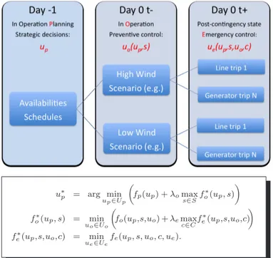
Figure 1 sketches how day-ahead operation planning under uncertainty may be formalized in the form of a three stage sequential decision making problem, where the successive stages correspond to different decision variables, namely
• up ∈ Up, denotes the strategic planning decisions that must be taken the day ahead (or possibly postponed) such as reserve purchase and/or maintenance rescheduling; • uo∈ Uo, denotes the preventive control actions that may
be taken in normal operation to ensure security, such as topology switching, generation rescheduling, Var-control; • ue ∈ Ue, represents corrective controls that may be applied in emergency mode, after the occurrence of a contingency (e.g. fast generation control, load shedding). In combination with these decision steps, the figure describes the possible future system states in the form of a tree, where the successive branchings correspond to the exogenous factors influencing the system state, namely
• scenarios s ∈ S, where S represents typically the uncer-tainty about power injections for the next day;
• contingencies c ∈ C, where C typically represents a list of generator or line trips, defining security criteria. Once the sets Up, S, Uo, C and Ue are well defined in this setting, the task of the operation planning engineer is to choose up ∈ Up such that for each scenario s ∈ S the best combination of preventive controls uo(up, s) ∈ Uo(dependent on the decision up and scenario s) and of corrective post-contingency controls ue(up, s, uo, c) ∈ Ue (also dependent on the contingency c and on the selected preventive control
uo) lead to an acceptable system performance. This task may be abstractly formulated as a three-level min-max problem described by the three equations of Figure 1, where
• the bottom equation models the task of emergency (contingency) control, as a minimization of post-contingency system degradation (measured by the func-tion fe) w.r.t. to ue; fein this equation could incorporate hard and soft constraints to model the acceptability of emergency mode behavior of power systems,
• the central equation models preventive control, as a tradeoff controlled by λe between costs and constraints of preventive control (measured by function fo) and of the worst-case post-contingency degradation, and, • the top equation models the operation planning decision
making problem, in the form of trading off the cost of strategic decisions upand security of operation under the worst-case scenario, a tradeoff controlled by λo.
Obviously, the formulation may be rephrased for modeling in-traday operation, and it could also be extended by introducing additional intermediate decision steps, but the essence of the problem is captured by this formalization.
u∗p = arg minu p∈Up µ fp(up) + λomax s∈Sf ∗ o(up, s) ¶ f∗ o(up, s) = min uo∈Uo µ fo(up,s,uo) + λemax c∈Cf ∗ e(up,s,uo,c) ¶ f∗ e(up,s,uo,c) = min ue∈Ue fe(up, s, uo, c, ue).
Fig. 1. Schematic overview of the three-stage decision making process under uncertainties (here applied to day-ahead operation planning)
To precisely define the above problem, the sets Up, Uo, Ue, the functions fp, fo, fe, and the uncertainty sets C and S must be chosen. In this context, a main difficulty is to define the set S of uncertain scenarios to be covered by operation planning decisions. In the following subsections we focus on this question and provide some tractable mathematical pro-gramming formulations addressing it. Our formulations also aim at formalizing the problem solving strategy of operation planning engineers. We present them by gradually reducing the formulation of Figure 1 to simpler subproblems.
IV. PRACTICAL SOLUTION APPROACHES
The abstract formulation of Section III expresses in a compact and very generic fashion the general problem of operation planning and intraday operation under uncertainty. The compact nature of this problem formulation however hides the huge algorithmic complexity of the underlying family of optimization problems which, as a matter of fact, are currently not amenable to an exact solution for large-scale power systems with realistic computing resources. This formulation also hides the fact that in practice the a priori specification of a relevant set S of uncertain scenarios is difficult.
In order to provide computationally realistic approaches, potentially useful in practice, we propose in the following subsections adaptations simplifying (or relaxing) the overall problem, so as to derive scalable optimization strategies that may help to construct approximate solutions to this overall problem with reasonable amounts of computing resources, and help to define appropriate uncertainty sets S.
A. Day ahead feasibility checking instead of optimization
The first, important, simplification that we propose is to explicitly reduce the day ahead (upper layer) optimization problem to a feasibility checking problem rather than an opti-mization problem. Thus, we propose that instead of searching for an optimal day ahead decision u∗
pas defined in Figure 1, it is more productive to consider the problem of checking for a given day ahead decision (say ¯up) whether or not the system security will be manageable for the next day.
In other words, we ask whether or not for all scenarios
s ∈ S, the possible combinations of preventive and corrective
controls enabled by ¯up will be sufficient to maintain the system in acceptable conditions during the next day, even if they would be very costly. Mathematically, we formulate this problem in the following way:
max s minu | δ | (1) s.t. s ∈ S u ∈ (Uo)T × (Uc)T |C| F (x, u, s) = 0 C(x, u, s) ≤ δL, where
• for notational simplicity we have dropped the dependence of the problem on the given value of ¯up;
• u ∈ (Uo)T × (Uc)T |C| denotes the vector of preventive and corrective control decisions, T being the number of time steps used to model the next day operation and | C | the number of contingencies;
• x ∈ (X)T × (X)T |C| is a vector of state variables jointly representing the possible pre-contingency and post-contingency states of the system at each time step and for each contingency (X denotes the state space of the power system);
• the vector function F (x, u, s) models the power balance equations in the pre-contingency and also in the post-contingency states implied for each time step by any element c ∈ C;
• the vector function C(x, u, s) and vector of limits L model similarly the pre- and post-contingency constraints that need to be satisfied at every time step, for every scenario, and for each contingency;
• δ is a vector of “slack” variables ensuring feasibility of the mathematical problem by multiplying component-wise the vector of limits L; if some of its components at the optimum are larger than 1 this means that the operational problem is not feasible;
• we have, for the sake of simplicity, dropped the dynamic constraints that link preventive and corrective controls at different time steps;
• s ∈ S, where S describes the uncertainties about the pos-sible scenarios. Notice that uncertainties are in practice described by at set of possible time series ranging over the considered decision horizon {t ≤ T }.
B. Discussion
This problem formulation1 aims at checking whether for
the given choice of decisions ¯up and for any scenario s ∈ S there would exist combinations of next day preventive and corrective control actions to ensure security with respect to all contingencies c ∈ C, given the available control means.
At this stage, it is important to notice that the hard equality constraints F (x, u, s) = 0, which are imposed in our mathe-matical problem formulation of Eqn (1), will implicitly restrict the consideration of the subset ¯S(F, Uo, Ue) ⊂ S of scenarios for which these constraints may be satisfied given the physical model (defined by the power balance equations F ) and the hard constraints on control resources defined by Uo and Ue. Thus, the solutions s∗ defined by Eqn (1) actually correspond to the most constraining scenarios in S among the subset ¯S
of those that are still compatible with the existence of an equilibrium (pre-contingency, and post-contingency for each
c ∈ C) as imposed by F (x, u, s) = 0.
At first sight, this formulation may seem restrictive and counterintuitive, since imposing the constraints F (x, u, s) = 0 is tantamount to shadowing the seemingly worst subset of scenarios out of the optimization problem, i.e. those for which the basic physical laws can not be respected anymore. On the contrary, we believe that it is actually very reasonable and, as a matter of fact, essential to impose these physical feasibility constraints on the subset of uncertain scenarios that should be considered in the decision making procedure. Indeed, the existence of scenarios in S for which the physical model is not satisfiable would mean that either the physical model F or the uncertainty set S are to be questioned. Although we will not pursue along this direction in this paper, let us notice that it is possible to formulate alternative optimization problems by removing the inequality constraints C and relaxing the equality constraints F instead, in order to explicitly check for the incompatibility of the physical model F and the postulated uncertainty set S.
On the other hand, the relaxation of the security constraints
C(x, u, s) ≤ L together with the used objective function imply
that, if the optimal values of all components of the vector δ are not larger than 1, then for all those scenarios in S which are compatible with the existence of a control strategy ensuring
F (x, u, s) = 0, also the security limits may be respected.
If this is not the case, it means that there exist scenarios which are not manageable by using solely the preventive and emergency control resources during the next day; thus the planning engineer will have to find substitutes for ¯up in order to ensure feasibility of the problem with δ ≤ 1.
The solution of problem (1) provides the most constraining scenario(s) s∗; they may be used to find alternative decisions ˜
up 6= ¯up (if δ∗ > 1), or to alert operators. The search for decisions ˜up and operation are greatly facilitated, once the worst scenarios have been identified.
1To fix ideas, if we consider a power system with on the order of N elements (lines or nodes), we will have | C |= O(N ) and dim(Uo) = O(N )
as well as dim(Uc) = O(N ) and dim(X) = O(N ). Thus the size of the
space within which the above optimization problem is formulated is O(T N2). For the sake of simplicity, we will assume in the rest of this paper that T = 1, and hence drop the time index form our notations.
C. Problem decomposition
To have a well-conditioned optimization problem, it is a bad idea to mix different types of constraints for example overload and voltage constraints that would lead to conflicting objectives and hence yield multiple local optima of the global problem defined by equation (1), and among which it would be very difficult to extract one single meaningful worst-case scenario s∗ for subsequent decision making.
Thus, in a practical implementation, we suggest to decom-pose the overall problem into physical subproblems and to compute separately a set of worst-case scenarios correspond-ing to these different physical subproblems. Notice that since we focus on feasibility rather than optimization at this stage, such a decomposition makes sense. Indeed, if all physical subproblems are feasible, then the overall problem is feasible as well. On the other hand, if we identify several subproblems that need a change of the value ˜up to become feasible, we believe that the problem of finding a single new ˜up that complies with all constraints for all the identified constraining scenarios is manageable by engineering expertise.
Concerning the set of inequality constraints C(x, u, s) in Eqn (1), we can as well choose among different options. Thus, we could reduce δ to a scalar variable in (1) or, for a given subproblem, restrict the set of constraints to a subset of constraints that are related to an a priori known weak-point of the system for that subproblem. In this latter case, we would model the fact that δ∗ should only be impacted by a single (or a small number of) a priori given and “comparable” constraints
Ck, by replacing the overall vector of inequality constraints by some constraints of the type
Ck(x, u, s) ≤ δLk. (2)
The general objective formulated by equation (1) takes into account a set of contingencies and deals with the computation of the associated corrective actions. Even with the above sug-gested reductions, it remains a very huge problem impossible to solve for large-scale power systems. In the next section we consider implementations of solution approaches, and to this end we propose to solve the problem separately for each single contingency. The results are then the preventive and corrective actions and most constraining scenario for each contingency. If several contingencies require preventive actions, we normally need to compute the common optimal set of preventive actions but, again, as our main objective is to check the feasibility, we only need to find a possible common set of preventive actions. Building on these ideas, we the following section presents a possible implementation to solve this problem in the restricted context of line overload constraints.
V. PREVENTIVE/CORRECTIVE ACTIONS ASSOCIATED TO LINE OVERLOAD PROBLEMS
For line overload problems, it is possible to find a practical implementation which determines extreme scenarios given the strategic decisions. The solution strategy that we propose determines u∗
o and u∗e and s∗ for each contingency c in C with the algorithm given in Table I.
TABLE I
ALGORITHM FOR SEPARATELY COVERING SINGLE CONTINGENCIES
do (for a given contingency c ∈ C): 1) determine a worst case scenario s?
c(¯uo) associated to c based on using
only corrective controls (problem (3) with ¯uo fixed a priori) and its
corresponding value of δ?(c, ¯u o);
2) if preventive controls changes are required for contingency c (i.e. if δ?(c, ¯u
o) ≥ 1), determine u?o(c), u?e(c), V?(c), Vpost? (c) s.t. : • the preventive control change ∆uo= uo− ¯uois minimized, • preventive constraints C(V, uo, s?c(¯uo)) ≤ Loare enforced, • emergency constraints Cpost(Vpost, uo, ue, s?c(¯uo)) ≤ Le are
also enforced. foreach contingency c in C. where
• Lo, Le denote respectively security thresholds in the preventive state
and in the emergency state. (The system state can remain indefinitely below limit Lo, and about Teseconds below Le.)
• V , Vpost stand respectively for the complex voltage vectors “before c and ue”, “after c and ue” and match the nodal power balances F (V, uo, s) = 0, Fpost(Vpost, uo, ue, s) = 0.
In this procedure, the first step consists of determining for a contingency c the worst-case scenario by checking whether by using only emergency control resources the problem is indeed manageable. We formulate this problem in the following way as a bi-level mathematical programming problem:
δ?(c, ¯uo) = max δ (3) s.t. s ∈ S C(V, ¯uo, s) ≤ Lo F (V, ¯uo, s) = 0 δ ≤ δ? c (δc?, u?e) = arg min (δc,ue) δc s.t. ue∈ Ue Cpost(Vpost, ¯uo, ue, s) ≤ δcLe Fpost(Vpost, ¯uo, ue, s) = 0.
In problem (3) the preventive control ¯uo ∈ Uo is a fixed parameter, and the constraints C(V, ¯uo, s) ≤ Lo and
F (V, ¯uo, s) = 0 are imposed over the set of possible scenarios, thereby restricting them to those that will lead to realistic and viable pre-contingency states.
If problem (3) leads to a value of δ?(c, ¯uo) > 1, it means that for contingency c there are some scenarios for which security can not be managed only via emergency control. Adjustment of preventive controls are then computed in the second step of the algorithm, based on the most constraining scenario s∗
c(¯uo) identified at the first step. If during this second optimization process, the problem is unfeasible (for at least one contingency), adjustment of strategic decisions up are required.
Notice that the determination of the worst uncertainty pat-tern for a contingency requires defining a measure to quantify the worst operating conditions. A natural choice is to express the worst operating conditions in terms of the maximum overall amount of post-contingency constraint violations (e.g. branch overloads).
The procedure described in this section decomposes the security analysis problem under uncertain scenarios into sub-problems formulated with respect to a single contingency; in-deed, if at least one of these contingency specific optimization problems turns out to have no solution combining preventive and emergency controls covering all uncertain scenarios, it reveals that day ahead strategic decisions must be taken. In this paper, for sake of simplicity, we do not consider the adjustment of preventive controls to the realization of uncertain scenarios, which would be mandatory in order to claim that the system state is “safe”. Our definition of safety means that for all uncertain scenarios, after implementing preventive and corrective actions, all the constraints are satisfied for all contingencies.
On the other hand, even if each subproblem posed for each contingency is found to have a satisfactory solution combining preventive and emergency controls, it does not yet imply the existence of a single preventive control decision common to all preventively feasible (and preventively secure) scenarios that is able to ensure that for all these scenarios all contingencies may be covered by their associated emergency control actions. We leave these two questions of “synchronizing” the preventive control decisions with uncertainties and contingencies for future research.
A. Discussion
Each worst-case scenario, regardless of its association to a contingency, contains a degree of arbitrariness, due to the choice of the criteria to be maximized. Nevertheless, it is possible to identify two characteristics that are, arguably, reasonable and necessary.
Consider the value of the objective function of (3) at the optimum as determined by the choice of the sets S and Ue; in general this value should increase with the size of the uncertainty set S and decrease with the size of the emergency control action set Ue. More precisely, the following two properties should hold true:
S0 ⊂ S ⇒ δ∗(S0, Ue) ≤ δ∗(S, Ue), (4)
U0
e⊂ Ue⇒ δ∗(S, Ue0) ≥ δ∗(S, Ue). (5) In the most general case (i.e. AC power system model), to ensure the property (4), we must suppose that a non linear max/min algorithm can always reach the global optimum. But this may not even be sufficient to obtain the property (5). Suppose, for instance, that, for a given s0 ∈ S, the constraint
Fpost(Vpost, u0, ue, s0) = 0 is feasible for some ue ∈ Ue but not for any ue∈ U0
e. It means that the value s = s0 has never been considered in the calculation of δ∗(S, U0
e), so nothing guarantees that the global optimum δ∗(S, Ue) does not occur at s = s0 with δ∗(S, U0
e) < δ∗(S, Ue).
As mentioned in [1], problem (3) describes two decision makers: the leader who controls the variables δ and s and the follower who controls the remaining variables. Both have their own objective function and constraints. The follower’s decisions depend on the leader’s decisions, but are not re-strained by the leader’s constraints. It is prohibited for the
leader to make decisions that would violate his constraints, when combined with the follower’s decisions.
VI. HOW TO FURTHER SIMPLIFY THE PROBLEM? When the problem (3) is expressed only through linear relations (i.e. if functions F and C are obtained from the DC approximation, and if the set S of scenarios and the set Ueof possible emergency controls are linearly constrained subsets of some vector space), it falls in the linear max-min problem category ([1]) in which the objective function of the follower is the opposite of that of the leader and in which the second-level variables do not appear in the first second-level constraints
C(V, u0, s) ≤ L0and F (V, u0, s) = 0.
Moreover, two very nice features appear in the linear case. Indeed, (i) the formulation of (3) makes the follower problem always feasible and (ii) the global optimum can be obtained thanks to an equivalence of the optimization problem with a manageable MILP (Mixed Integer Linear Programming) problem for which standard solvers do exist. Consequently, in the linear case the formulation turns as well out to meet the requirements (4) and (5) discussed above.
Indeed, in the linear case, problem (3) can be generically written in the following fashion:
max x,y c 1tx + d1ty s.t. A1x + B1y ≤ 0, x ≥ 0, y ∈ arg max y c 2tx + d2ty, s.t. A2x + B2y ≤ 0, y ≥ 0, (6)
which is equivalent to the classical linear complementary problem (7): max e x ec ex s.t. Aeex ≤ 0, M ex + q ≥ 0, ex ≥ 0 e xt(M ex + q) = 0. (7) where e x = xy λ eb = b1 ec = c 1 d1 0 q = −d02 b2 (8) e A =£A1 B1 0¤ M = 00 00 B02t −A2 −B2 0 (9) We can solve (7) due to the property: there exist a large constant L > 0 such that each solution of (7) is a solution of the MILP problem (10):
max e x ec ex s.t. Aeex ≤ 0, e x ≥ 0, M ex + q ≥ 0 e x ≤ Lu, M ex + q ≤ L(1 − u) u binary vector (10)
The matrices A1, A2, B1, B2 and the vectors c1, c2, d1, d2
are detailed in the appendix, where the proof provided by [1] is summarized.
VII. NUMERICAL SIMULATIONS
To illustrate the ideas exposed in this paper, we use two examples built with two small transmission networks.
We first consider a simple 7-bus system where the outage of a line requires both preventive and emergency control actions in order to cover the worst-case scenario.
Next, we use a modified version of the IEEE 30-bus system, to illustrate a situation where in the worst-case there exists no combination of preventive and corrective actions that solve the problem, thus requiring the call for strategic day ahead decisions.
A. 7-bus system
Figure 2 shows a simple 7-bus system that we have designed for the purpose for this paper.
Two generators (labels u1
o and u2o) are committed to supply a load (P2). All line current thresholds Loand Leare
respec-tively fixed to 30 and 40 p.u. There are two phase-shifting transformers (u1
e and u2e).
We study a contingency corresponding to the outage of the dashed line of Fig. 2 with respect to the uncertainties induced by the power injections s1, . . . , s4. In our simulations the range
of uncertainties is limited only by the set of system constraints in preventive mode, which implies that the power balance remains satisfied (i.e. s1+ s2 + s3+ s4 = 0) and that the
permanent power flow limits Lo are respected.
2
s
1 eu
2 eu
3s
s
4 1s
1 ou
2P
2 ou
Fig. 2. 7-bus system with uncertain nodal injections, represented by the variables s1, s2, s3, s4
In our illustration, we suppose that preventive control deci-sions u1
oand u2ocorrespond to the changes of the two generator
schedules, while the emergency control decisions u1
e and u2e
correspond to the phase shifts of the two transformers (see Fig. 2). To construct a base we have determined a configuration of values si saturating the preventive security constraints. The
corresponding scenario s∗
o is given in Table II (we will denote
the associated preventive control settings by ¯uo).
Table III provides the results (in terms of degree of post-contingency constraint violations) of three successive simu-lations. In the first line, we kept ∆uo = 0 (uo frozen to its
value ¯uo), and ∆ue= 0 (no emergency control resources); the
smin smax s1 s2 s3 s4
−103 +103 −40 +66.66 −40 13.33
value of δ reflects the post-contingency constraint violations for a worst-case scenario s∗
1, when preventive controls are
adjusted to cover the worst preventively acceptable scenario and no emergency control is used later on. In the second line, we still assume that ∆uo = 0, but allow emergency
controls (phase shifters) to react optimally to scenarios. The value of δ > 1 shows that the even under emergency control, there is a scenario s∗
2 that is preventively secure but still
leads to unmanageable post-contingency constraints. Finally, the last line of the table shows the result when the latter scenario s∗
2 is frozen to the value computed at the previous
stage, and when we search for a combination of preventive and emergency controls to satisfy both preventive and post-contingency constraints given this scenario, while minimizing the deviation of uo with respect to ¯uo. It shows that the
scenario s∗
2 may be covered by a combination of preventive
and corrective controls.
We observe that in this problem it was necessary to call for a combination of preventive and emergency controls to cope with the worst scenario.
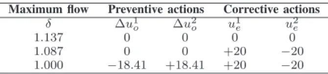
TABLE III
7-BUS SYSTEM:WORST-CASE SITUATION ASSOCIATED TO THE OUTAGE OF THE DASHED LINE
Maximum flow Preventive actions Corrective actions
δ ∆u1
o ∆u2o u1e u2e
1.137 0 0 0 0
1.087 0 0 +20 −20
1.000 −18.41 +18.41 +20 −20
Phase shifter transformers upper and lower bounds (+20 and -20 degrees) are all reached on this example, as indicated by the columns u1
eand u2eof Table III. The maximum flow values,
before and after outage of the dashed line, occur on the left horizontal line on Fig. 2.
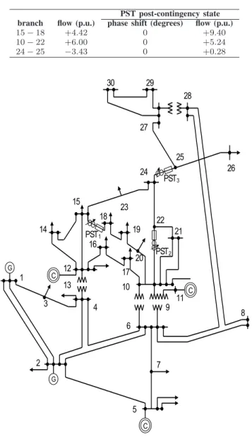
B. 30-bus system
Our second illustration is based on the IEEE 30-bus system depicted on Figure 3. We have upgraded the system with three phase-shifting transformers (PSTs) as shown on the one-line diagram of Figure 3. Their location is inspired by Reference [10], which suggests that these are the optimal locations for placing a small number of PSTs in this system. The three (identical) PSTs have thus been installed in series with the lines originally defining the branches 15-18, 10-22 and 24-25. We supposed that their phase shift ranges for our illustration should be constrained to +/-20 degrees.
In our analysis, we consider again a single contingency, namely the outage of line 4-6, and we suppose that security constraints apply only on the currents of the lines where a PST is installed, with the limits Lo, Le respectively fixed to the
independent variations of all the loads at all the buses in the range [-20%,+20%] from their base case value.
We made a first simulation without using any post-contingency controls while using the possibility to reschedule generation power in the pre-contingency state. The results are given in Table IV.
TABLE IV
30-BUS SYSTEM:WORST-CASE SITUATION ASSOCIATED TO THE BRANCH OUTAGE4-6WITHOUT ACTION OFPST
PST post-contingency state branch flow (p.u.) phase shift (degrees) flow (p.u.)
15 − 18 +4.42 0 +9.40
10 − 22 +6.00 0 +5.24
24 − 25 −3.43 0 +0.28
Fig. 3. Modified IEEE 30-bus system; adapted by adding three phase-shifting tranformers
These results show that (see first line), in the worst case the branch 15-18 will be severely overloaded if no post-contingency controls are solicited.
In order to see whether a combination of preventive and emergency controls could solve the problem, we applied the full procedure of Table I to this problem. The resulting optimum is described in Table V. We observe that the problem is still ‘infeasible’ since the solution leads to current flows on branch 15-18 which are still above the acceptable limit of 7.2 (see first line), while the current at the optimum in line 10-22 has been increased with respect to the result of Table IV.
TABLE V
30-BUS SYSTEM:WORST-CASE SITUATION ASSOCIATED TO THE BRANCH OUTAGE4-6WHENPSTACT
PST post-contingency state branch flow (p.u.) phase shift (degrees) flow (p.u.)
15 − 18 +4.42 +20 +8.35
10 − 22 +6.00 −20 +6.74
24 − 25 −3.43 +20 −0.49
The latter example provides an illustration of a case where, without changing the strategic decisions up, it is not possible
to ensure system security for at least one contingency and for the worst scenario for this contingency.
VIII. RELATED WORKS
So far the worst-case operating conditions of a power system under operational uncertainty have been tackled in the literature in the framework of security margins [2], [4], [5], [3]. These approaches look for computing minimum security margins under operational uncertainty with respect to either thermal overload [5], [3] or voltage instability [2], [4], [5]. These approaches belong to the class of min-max optimization problems since a security margin represents by definition the maximum value of a so-called loading parameter for a given path of system evolution.
Ref. [2] computes the closest infeasibility to a given op-erating point by defining the feasible region in the power injection space as the set of all power injections for which the load flow equations have a solution. A minimum margin is defined and computed using the constrained Fletcher-Powell minimization. Ref. [4] proposes an iterative and a direct method to compute the locally closest saddle-node bifurcation to the current operating point in the load power parameter space. The Euclidian distance is used to compute the worst-case load increase causing the system to lose equilibrium. Ref. [5] extracts information from unstable voltage trajectories, such as the left eigenvector to the point of collapse, in order to iteratively “redirect” the worst uncertainty pattern.
The case where the feasible region is bounded by inequality constraints stemming from branch current limits (instead of bifurcations as for voltage instability) is considered in [5], [3]. Ref. [3] proposes a method to find the thermal-constrained interface maximum transfer capability under the worst scenario in generation-load space. The min-max interface transfer is obtained as a bi-level optimization problem whose constrains are derived from the DC load flow equations. The bi-level optimization problem is solved by the branch and bound method. Ref. [5] computes minimal thermal security margins by using a heuristic enumerative approach which relies on the sensitivities of branch currents with respect to uncertain parameters.
IX. CONCLUSION
In this paper we have analyzed the task of dealing with un-certainties for security management of electric power systems in an integrated way from day-ahead to real-time, with the objective of proposing a unified framework and deriving opti-mization problem formulations to make this problem amenable to practicable solutions.
In our understanding, the problem faced by operation planning engineers is essentially a feasibility problem: they must check and ascertain the day ahead that the next day the operators will be able to manage the system security with the control resources they will dispose of, even in the worst possible scenario, given a reasonable definition of the uncertainty set that needs to be covered.
Uncertainty sets, in this context, are composed of combina-tions of operating scenarios and contingencies. The definition, in a rational way, of the operating scenarios and the contin-gencies, that need to be ‘covered’ in power system operation is a matter of debate, and in this paper we did not intend to provide any direct guidelines to chose them. Rather, we have proposed a framework for assessing security and deriving decision strategies, once these sets are provided.
We have proposed a generic ‘min-max-min’ formulation of the day-ahead security control problem, which highlights the role played by uncertain scenarios about operating conditions that need to be taken into account, as well as the constraints imposed by contingency sets used to define security of oper-ation.
Since, with current computational resources and state-of-the-art optimization methods, this overall problem is not practically solvable for large scale power systems, we have proposed in this paper a sequence of problem simplifications which make it possible to find solutions of very much simpli-fied versions (e.g. by considering only a single contingency at the time and by restricting to problems of branch overloads) to determine a reasonable worst-case scenario and its associated combination of preventive and emergency controls. While limited in scope, the resulting algorithms already constitute a significant progress, since they allow to identify constraining scenarios for the next day in a systematic way.
We have left open voltage stability and dynamic security problems and the difficulty of finding a single preventive con-trol strategy able to cover several contingencies and instability phenomena.
Future work will be based on looking back at the overall problem as a huge simultaneous constraint satisfaction prob-lem over combinations of “scenarios”, “contingencies”, and constraining power system “elements”.
We indeed believe that looking at this problem in a very global way may provide new insights and suggest new possible solution strategies based on the analysis of the correspondingly very large number of possible problem relaxations.
ACKNOWLEDGMENTS
This paper presents research results of the European FP7 project PEGASE. Louis Wehenkel acknowledges the support of the Belgian Network DYSCO (Dynamical Systems, Control, and Optimization), funded by the Interuniversity Attraction Poles Programme, initiated by the Belgian State, Science Policy Office. The scientific responsi-bility rests with the authors.
REFERENCES
[1] C. Audet, P. Hansen, B. Jaumard, and G. Savard, “Links between linear bilevel and mixed 0-1 programming problems”, Journal of Optimization
Theory and Applications, vol. 93, no. 2,
[2] J. Jarjis and F.D. Galiana, “Quantitative analysis of steady state stability in power networks”, IEEE Trans. on Power Apparatus and Systems, vol. PAS-100, no. 1, 1981, pp. 318-326.
[3] D. Gan, X. Luo, D.V. Bourcier, and R.J. Thomas, “Min-Max Transfer Capability of Transmission Interfaces”, International Journal of Electrical
Power and Energy Systems, vol.25, no. 5, 2003, pp. 347-353.
[4] I. Dobson and L. Lu, “New methods for computing a closest saddle node bifurcation and worst case load power margin for voltage collapse”, IEEE
Trans. on Power Systems, vol. 8, no. 2, 1993, pp. 905-911.
[5] F. Capitanescu and T. Van Cutsem, “Evaluating bounds on voltage and thermal security margins under power transfer uncertainty”, Proc. of the
14th PSCC Conference, Seville (Spain), June 2002.
[6] A. Motto, J. M. Arroyo, and F. D. Galiana, “A Mixed-Integer LP Procedure for the Analysis of Electric Grid Security under Disruptive Threat”, IEEE Trans. on Power Systems, vol. 20, no. 3, 2005, pp. 1357-1365.
[7] J. M. Arroyo and F. D. Galiana, “On the Solution of the Bilevel Programming Formulation of the Terrorist Threat Problem”, IEEE Trans.
on Power Systems, vol. 20, no. 2, pp. 789-797, May 2005.
[8] M.L. Latorre and S. Granville, “The Stackelberg equilibrium applied to AC power systems - a non-interior point algorithm”, IEEE Trans. Power
Syst. vol. 18, no. 2, 2003, pp. 611-618.
[9] A.L. Motto and F.D. Galiana, “Coordination in markets with nonconvex-ities as a mathematical program with equilibrium constraints - Part I and II”, IEEE Trans. Power Syst., vol. 19, no. 1, 2004, pp. 309-324. [10] J.A. Momoh, J.Z. Zhu, G.D. Boswell and S. Hoffman, “Power System
Security Enhancement by OPF with Phase Shifter”, IEEE Trans. Power
Syst. vol. 16, no. 2, 2001, pp 287-293.
APPENDIXA
BILEVEL ANDMIXEDLINEARPROBLEMFORMULATIONS
From the definition of problem (3), the unknown vectors of the BLP problem encompass :
• x, the pre-contingency phase angles and uncertainties ex-pressed as variations of nodal active loads or generations • y, the scalar variable δ(= δc), the post-contingency phase angles and dummy injections representing the phase shifters
The max/min behaviour is obtained by fixing c1 = c2 = 0
and taking d1 = −d2 such that d1tx = δ. While the leader
constraint A1x ≤ 0 models the pre-contingency nodal power
balances and maintain in absolute value the flows below L0
(without any action of the PST since B1 = 0), the follower
constraint A2x + B2y ≤ 0 models the post-contingency nodal
power balances and the fact that the absolute value of the flows are lower than δL1. The remaining components of x
and y are positive slack variables used to enforce via the matrices A1, A2the validity ranges of angle and active power
quantities. The second-level problem of (6) has been replaced in (7) by its complementary slackness conditions where the dual variables are denoted by λ. The strong duality theorem states that if either the primal or dual problem has a finite optimal solution so does the other. The specific form of (6) deduced from (3) makes finite each feasible couple (x,y), it follows that each optimal solution ex? is bounded, so the constant L = max(kex?k
∞, kM ex?+qk∞) always exists. If we denote by eu? the vector whose the i-th component is equal to one if ex?
i > 0 and zero otherwise, (ex?,eu?) is a feasible solution of (10). Conversely, each feasible solution of (10) satisfies the constraint xt(M x + q) = 0. It implies that the optimal objective function values of the problems (6), (7), (10) are equal when L is large enough ( for instance, L is fixed to 103