Stochastic multi-scale modelling of MEMS

(1)

Aerospace and Mechanical Engineering Department Computational & Multiscale Mechanics of Materials

Stochastic multi-scale modelling

of MEMS

Thesis submitted in fulfilment of the requirements for the degree of Doctor in Engineering Sciences

by

Vincent Lucas, Ir.

(2)

(3)

Members of the Examination Committee

Prof. Jean-Claude GOLINVAL (President of the Committee) University of Li`ege (Li`ege, Belgium)

Email: jc.golinval@ulg.ac.be Prof. Ludovic NOELS (Advisor) University of Li`ege (Li`ege, Belgium) Email: l.noels@ulg.ac.be

Prof. Julien YVONNET

Universit´e Paris-Est Marne-La-Valle (Paris, France) Prof. Dirk VANDEPITTE

Katholieke Universiteit Leuven (Leuven, Belgium) Prof. Maarten ARNST

University of Li`ege (Li`ege, Belgium)

Dr. Ling WU (guest Professor at Vrije Universiteit Brussel (VUB), Brussels, Belgium)

(4)

(5)

Abstract

When studying Micro-Electro-Mechanical Systems (or MEMS) made of poly-crystalline materials, as the size of the device is only one or two orders of magnitude higher than the size of the grains, the structural properties exhibit a scatter at the macro-scale due to the existing randomness in the grain size, grain orientation, surface roughness... In order to predict the probabilistic be-haviour at the structural scale, we investigated the recourse to a stochastic 3-scale approach in this thesis dissertation.

Estimating the scatter in the response of the structure is studied at macro-scale based on stochastic finite elements along with Monte-Carlo simulations. To produce accurate results, the mesh size of the finite element approach should be small enough so that the heterogeneities can be captured. This can lead to overwhelming computation if the microstructure is directly considered, thus jus-tifying the recourse to stochastic homogenisation to define a meso-scale random field. Based on a stochastic model of this random field, the variability of the response of the structure can be computed.

In this work, the micro-scale uncertainties are modelled based on measure-ments provided by the IMT-Bucharest institute. These uncertainties are then propagated towards the macro-scale for 3 different problems. The first one serves the purpose of verification. The variability of the resonance frequency of a micro-beam is computed and compared to a reference numerical solution. The second problem extends the 3-scale approach to the thermo-elastic case. Thus the uncertainties of the quality factor of 3D beams are studied with a modelling of the anchor. Finally, the third problem aims at propagating surface roughness uncertainties on the resonance frequency of thin plates.

(6)

(7)

Acknowledgements

First, I want to thank Professors Jean-Claude Golinval, Dirk Vandepitte, Julien Yvonnet, Maarten Arnst, Ling Wu and Ludovic Noels who accepted to partici-pate in the examination committee of this doctoral thesis.

The research has been funded by the Walloon Region under the agreement no 1117477 (CT-INT 2011-11-14) in the context of the ERA-NET MNT frame-work. Computational resources have been provided by the supercomputing fa-cilities of the Consortium des Équipements de Calcul Intensif en Fédération Wallonie Bruxelles (C ÉCI) funded by the Fond de la Recherche Scientifique de Belgique (FRS-FNRS).

I wish to thank all the members of the 3SMVIB project. I am truly grateful to Zygmunt for the warm welcome he granted us in Poland. I would like to thank Open-Engineering for welcoming me in their office, and more particularly, St´ephane, for his patience while I was loading. I am sure he will understand.

I also want to acknowledge Vinh for all the bedroom sharing, Van Dung for being so helpful, and Ling for surviving in the mess I had established in our office and of course for her everlasting invaluable help. I also want to acknowledge the help of Prof. Maarten Arnst and Prof. Jean-Claude Golinval for their good advice. Many thanks must go to my advisor, Prof. Ludovic Noels. This thesis would never have seen the light of day without him. Ludovic grants his students a considerable amount of time, which is, I believe, the most precious resource of all.

I wish to thank my friends for their never-ending support. Archimede needed a lever, I needed their smiles. Finally, my thoughts go to my family who coped with me all these years. And I won’t forget Delphine who supported me against all tides.

(8)

(9)

Introduction

1.1 Background and motivation

Nowadays, MEMS, or microelectromechanical systems, are well-established de-vices which involve low fabrication costs, large volume production, light and small products with a reasonable energy consumption. They can thus be found in many different applications, ranging from vehicles to medicine technology. Producing reliable MEMS can however be a challenging task when, for exam-ple, a high quality factor1 (and thus a higher accuracy) is sought. This is the case for RF-MEMS filters or resonant sensors. To produce such MEMS with a high quality factor, the different mechanisms which involve energy dissipa-tion need to be properly identified. While some dissipadissipa-tion mechanisms can be reduced through proper operating conditions, such as air damping, other mechanisms rely solely on the design, such as thermoelastic damping. A proper modelling of such intrinsic loss mechanisms would allow to define an efficient MEMS design process.

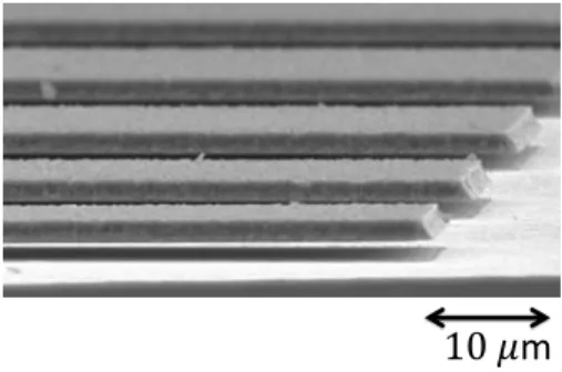
An efficient deterministic design however can be hazardous. From the de-sired design to produced MEMS, a non-negligible scatter in the device properties can be seen which can result in unusable MEMS. Such uncertainties, through the quality factor of micro-beams, are inevitable in MEMS design. Indeed, as MEMS involve small dimensions as well as complex systems, geometric uncer-tainties are unavoidable. The roughness of the different surfaces of the MEMS imply uncertainty. The material itself can also be subjected to uncertainties. For example it can be expressed through grain orientation of poly-crystalline materials with anisotropic crystals or through amorphous phase distribution when the crystallinity is not perfect. Fig. 1.1 illustrates such micro-beams, produced at the IMT institute in Bucharest.

With the help of uncertainty quantification (UQ) in MEMS design, parame-ters whose uncertainty should be controlled rigorously can be identified.

Consid-1_{A dimensionless parameter which characterises the bandwidth of a resonator as well as}

(14)

10 𝜇m

Figure 1.1: Samples of micro-beams, courtesy of IMT institute in Bucharest

ering UQ in the pre-design phase can lead to an efficient design whose success rate is satisfactory. However, the straightforward UQ method that could be applied, the Monte-Carlo procedure on the beam where each heterogeneities is modelled and meshed, is overwhelming in terms of computational resources. Therefore there are increasing interests into solving this problem in a more effi-cient way with a multi-scale method propagating the uncertainty. Investigating such an approach in the frame of MEMS design is the objective of this work.

1.2 Overview of the dissertation

In the micro-electromechanical systems (MEMS) community, there are increas-ing demands in developincreas-ing reliable micro-structures with very high quality fac-tors (Q). These micro-structures constitute the essential active part of applica-tions such as resonant sensors and RF-MEMS filters, for which increasing the sensitivity and resolution (a higher quality factor implies a lower bandwidth at resonant peaks) of the devices is a critical issue. In order to obtain high-Q micro-resonators, all dissipation mechanisms that contribute to decreasing the quality factor have to be identified and well considered at the design stage. The energy dissipation mechanisms of micro-resonators can be classified into two categories [100]. On the one hand, the majority of dissipation mechanisms are extrinsic, which means that they can be minimised by a proper design and oper-ating conditions, such as by minimising the air damping effect. Intrinsic losses, on the other hand, cannot be controlled as easily as extrinsic ones. Thermo-elastic damping has been identified as one kind of important intrinsic loss in high-Q micro-resonators [16, 34].

Thermo-elastic damping is an intrinsic energy dissipation mechanism which occurs due to heat conduction. In a thermo-elastic solid, the thermal and mechanical fields are strongly coupled through the thermal expansion effect. MEMS resonators generally contain elements which vibrate in flexural modes and can be approximated by beams. In a vibrating beam in its first flexu-ral mode, the two opposite sides undergo opposite deformations. When one

(15)

side is compressed and its temperature increases consequently, the other side is stretched with a decrease in the temperature. Thus temperature gradients are generated and an energy dissipation occurs. However, this dissipation has a measurable influence only when the vibration frequency is of the order of the thermal relaxation rate. On the one hand, when the vibration frequency is much lower than the thermal relaxation rate, the vibrations are isothermal since the solid is always in thermal equilibrium. On the other hand, when the vibration frequency is much higher than the thermal relaxation rate, the vibrations are adiabatic since the system has no time for thermal relaxation. In MEMS, due to the small dimensions involved, the relaxation times of both the mechanical and thermal fields have a similar order of magnitude and hence, thermo-elastic damping becomes important. Therefore, accurate modelling and prediction of energy loss due to the thermo-elastic effects becomes a key requirement in order to improve the performance of high-Q resonators.

The early studies of thermo-elastic damping were mainly based on analyt-ical models, which were derived for very simple structures and are subject to very restrictive assumptions. Zener [104] has developed the so-called Zener’s standard model to approximate thermo-elastic damping for flexural vibrations of thin rectangular beams. Based on an extension of Hooke’s law to the “Stan-dard Anelastic Solid”, which involves the stress σ, strain ε as well as their first time derivatives ˙σ, ˙ε, the vibration characteristics of the solid are analysed with the harmonic stress and strain. However Zener’s theory [104] does not provide the estimation of the frequency shift induced by thermo-elastic effects. For this purpose, Lifshitz and Roukes have developed in [50] the thermo-elastic equa-tions of a vibrating beam based on the same fundamental physics than Zener, which model more accurately the transverse temperature profile. The analytical models can be used to obtain the complex thermo-elastic resonant pulsation $n

and its corresponding quality factor Q for simplified cases only. The limitation of analytical models and the complexity of the real micro-structures (i.e. non rectangular geometry, complex 3-D structures, anisotropic material,...) have motivated the development of numerical models [48],[81], and the application of the finite element method to study the thermo-elastic damping has been validated by the comparisons of numerical results with analytical results.

However, deterministic finite element models are not accurate enough to obtain a reliable analysis of the performance of micro-resonators [48]. Indeed, MEMS are subject to inevitable and inherent uncertainties in their dimensional parameters and material properties which lead to variability in their perfor-mance and reliability. Due to the small dimensions of MEMS, manufacturing processes leave substantial variability in the shape and geometry of the device, while the material properties of a component are inherently subject to a scatter. The effects of these variations have to be considered and a stochastic modelling methodology is needed in order to ensure the required MEMS performance un-der uncertainties.

Sources of uncertainties are most of the time neglected in numerical models. However they can affect the structural behaviour, in which case it is important to consider them. This is why nowadays a lot of efforts are spent on

(16)

improv-ing uncertainty quantification procedures. Dealimprov-ing with uncertainties can be done in different ways, but this work focuses on the propagation of micro-scale material and geometrical uncertainties up to the structural response. Micro-scale material uncertainties result from spatially varying material properties. The structural behaviour is thus non-deterministic as the material properties are not homogeneous over the structure. This structure can be modelled using the finite element method, in which case a full description of the material het-erogeneities and of their variations is required. Using Monte-Carlo simulations on such a fine discretization to estimate the uncertainties in the structural be-haviour, i.e. performing direct Monte Carlo simulations, can however involve overwhelming computation cost as the finite element mesh should capture the micro-scale uncertainties. The purpose of this work is to investigate the recourse to stochastic methods to study the probabilistic behaviour of MEMS.

Stochastic Finite Elements methods, referred to as SFEM and described in [24, 47, 88], as a non exhaustive list, are relevant tools to study uncertainty quantification at a reasonable cost. In the case of MEMS, this was illustrated by considering thermoelastic stochastic finite elements in [48]. SFEM to study the stochastic behaviour of shells whose thickness and material properties are random was also used in [89]. However, with those approaches, the random field used to describe the spatially varying material properties and thickness was not obtained directly from micro-structure resolutions. Thus the recourse of SFEM approaches alone does not overcome the problem of modelling the material heterogeneities. Indeed, to be able to propagate the uncertainties from the micro-structure itself using SFEM, as the involved uncertainties are charac-terised by a small correlation length, the finite element size should be drastically reduced [84]. According to [28], accurate results are obtained when the finite element size is smaller than at least one half of the correlation length, which would lead to unreachable computational resources to capture the micro-scale heterogeneities uncertainties. However, this limitation can be overcome thanks to multi-scale approaches as the introduction of an intermediate scale implies a larger correlation length, and thus reduces the computation cost of the SFEM procedure [52].

Multi-scale approaches are an efficient, convenient and elegant way to deal with complex heterogeneous materials. The rise of composites, among other progresses in material science, led to an the extensive use of complex materi-als. The micro-structure of such materials can involve a mixture of different materials arranged according to a complex geometry. The numerical simula-tion of structures made of such materials requires insights of the behaviour of the micro-structure to produce accurate results. Including the modelling of the micro-structure in the frame of a direct simulation has a cost which can lead to an unaffordable computational burden. This is the starting point of multi-scale approaches where the macro scale simulation does not model the micro-structure directly but is informed of analyses performed at the micro-scale.

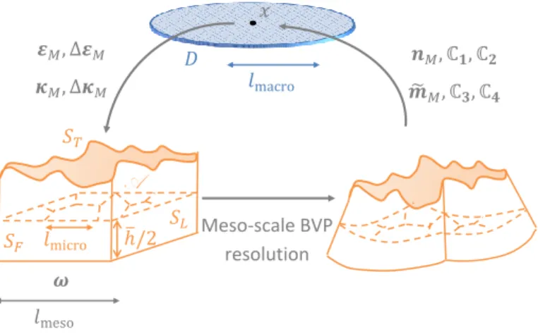
In such an analysis, three scales are defined, see Fig. 1.2. The micro-scale is the characteristic size of the micro-structure. A volume element made of the material of interest defines an intermediate scale: the meso-scale. The

(17)

macro-𝐷 𝑥 𝜺𝑀, Δ𝜺𝑀 𝝈𝑀, ℂ𝑴 𝑙macro 𝑥 Meso-scale BVP resolution 𝝎 =∪𝑖𝝎𝑖 𝑙meso 𝑙micro 𝑥

Figure 1.2: Homogenisation-based multi-scale method with 1st-order homogeni-sation for classical macro-scale continuum.

scale is the characteristic size of the whole structure, based on the gradient of the structural loading. A macro-scale problem is defined and solved nu-merically with usual methods such as an FE analysis. The resolution of this problem requires micro-scale information through homogenised properties at the meso-scale. Therefore the homogenisation itself is the cornerstone of several multi-scale approaches. On the one hand, when the homogenisation is done a priori, one refers to a sequential approach. On the other hand, when an ho-mogenisation procedure is called at various steps of the macro-scale solver, thus involving a coupling between the two problems, one refers to a concurrent ap-proach. In a concurrent approach, the strain information at any point of the macro-scale model can be down-scaled, analysed at the micro-scale to estimate a homogenised stress counterpart, which is then up-scaled to the macro-scale problem.

The multi-scale approach produces relevant results when some hypotheses are fulfilled. First, the method needs to be consistent: the deformation energy should be the same at both the micro and macro-scales. This condition is referred to as the Hill-Mandel condition. Second, the length scale separation which can be expressed as

lmeso<< lmacro, and (1.1)

lmicro<< lmeso, (1.2)

should be satisfied.

The first equation (1.1) guarantees the accuracy of the procedure: accurate results are obtained when the homogenisation is applied on meso-scale volume

(18)

elements whose size is much smaller than the characteristic length on which the macro-scale loading varies in space [21]. The second one, Eq. (1.2), ensures the RVE existence. RVE stands for representative volume element. A volume element is said to be representative when it is large enough to statistically represent the material of interest. In other words, the homogenised properties do not depend on the choice of volume element as well as they do not depend on the type of energetically consistent boundary conditions.

Following an energetically consistent approach and owing to both scale-separations, relevant results can be obtained with multi-scale methods. How-ever, the homogenisation procedure still needs to be defined. The homogeni-sation step can be done in many different ways. For example, semi-analytical methods exist, such as the mean-field homogenisation (MFH), whose starting point is Eshelby’s eigenstrains [18]. When the micro-structure is made of repet-itive unit cells, asymptotic homogenisation can be used to state the equations at different orders corresponding to the ratio between scales, and the resolution of the corresponding lower scale equations usually follows a unit cell resolution. The FE2 and FFT methods are numerical approaches which can compute ho-mogenised properties in a wide range of applications. A more detailled review of the state of the art is given in Section 3.1. Moreover, reviews of the different multi-scale approaches can be found in [40] for a general overview, in [22] for an emphasis on numerical approaches and in [51] for multi-scale approaches in the frame of damage.

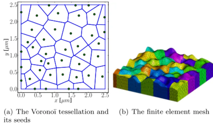
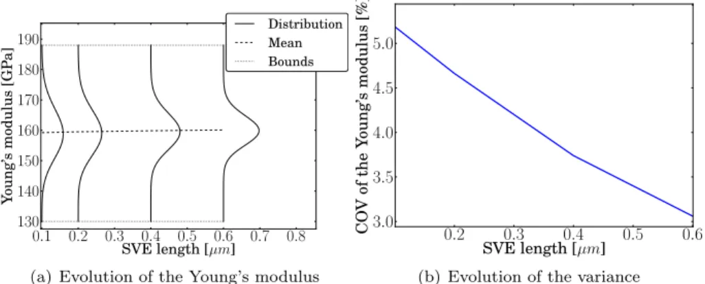
When dealing with reduced size structures, the characteristic size of the micro-scale heterogeneities can be too close to the macro-scale to respect both scale separations (1.1) and (1.2). The first one, Eq. (1.1), guarantees the accu-racy of the procedure. Therefore, it should be satisfied. The second scale sepa-ration, Eq. (1.2), will thus not be respected. This implies that volume elements are not representative and they are referred to as Statistical Volume Elements (SVEs) [70]. Indeed, on the one hand, the meso-scale boundary value problem over an SVE is boundary condition dependent, and on the other hand, differ-ent homogenised properties are obtained for differdiffer-ent realisations of the SVEs, even under a unique case of BCs. Although it is possible to address the lack of representativity by statistical considerations of the homogenised properties for different SVE sizes/realisations [39, 32] in order to extract mean homogenised properties or to define minimum RVE size, such a method does not allow to up-scale the uncertainties. This has motivated the development of stochastic multi-scale methods.

Stochastic multi-scale analyses have been developed based on order reduc-tion of asymptotic homogenisareduc-tion [20] to account for micro-scale material un-certainties in the form of random variables –and random fields in particular cases. However, accounting for general fine-scale random fields would require the nested solution of micro-scale problems during the structural-scale analysis, leading to a prohibitive cost. Local effects can be treated using Monte-Carlo simulations: the brittle failure of MEMS made of a poly-silicon material was studied by considering several realisations of a critical zone [55] on which the relevant loading was applied. An alternative to these approaches is to introduce

(19)

in the stochastic multi-scale method a meso-scale random field, obtained from a multi-scale analysis, in order to conduct the stochastic finite element method at the structural scale in an uncoupled way.

For this purpose, statistics and homogenisation were coupled to investigated the probability convergence criterion of RVE for masonry [27], to obtain the property variations due to the grain structure of poly-silicon film [54], to ex-tract the stochastic properties of the parameters of a meso-scale porous steel alloy material model [101], to evaluate open foams meso-scale properties [49], to extract probabilistic meso-scale cohesive laws for poly-silicon [65], to ex-tract effective properties of random two-phase composites [90], to study the scale-dependency of homogenisation for matrix-inclusion composites [92, 93], or again to consider the problem of composite materials under finite strains [53]. In this last reference, a particular attention was drawn on the correlation be-tween the different sources of uncertainty. In most of the previously cited works, the stochastic homogenisation on SVEs was mainly achieved by a combination of computational homogenisation with Monte Carlo simulation. In the recent works of [73], the stochastic homogenisation was achieved by using a modified version of the SFEM (here applied on the meso-scale boundary value problem), leading to a more efficient resolution. The problem of high-dimensionality was investigated in [9], in which the resolution of composite material elementary cells was used to explicitly define a meso-scale potential with the aim of studying the uncertainties in the fibers geometry/distribution in the case of finite elasticity.

The meso-scale uncertainties can then be up-scaled to study the probabilistic macro-scale behaviour. Based on their stochastic properties identification of the meso-scale porous steel alloy material model [101], Yin et al. [102] have generated a random field based on Karhunen-Lo`eve expansion to study the macro-scale behaviour. A similar approach was applied to study the dynamic behaviour of open-foamed structures [49].

The purpose of this thesis dissertation is to develop a stochastic 3-scale method applied on MEMS vibrating beams. The main steps of this approach can be summarised as (i) the definition of micro-scale SVEs with a random structure; (ii) at the meso-scale, finite-element simulations on different SVEs, defined from a larger material sample by using the moving window technique, lead to the distribution of the homogenised poly-crystalline material properties and their spatial correlation; (iii) a random field of the meso-scale homogenised properties is generated based on the information obtained from the SVE simu-lations; and (iv) the generated meso-scale random fields are used in the frame of a stochastic finite element method to predict the statistical distribution of MEMS macro scale properties of interest such as their resonant frequencies or their thermoelastic damping. In particular, by comparison with direct Monte-Carlo simulations, it will be shown that the generation of a spatially correlated random field allows predicting macro-scale statistical distributions which do not depend on the SVE size and macro-scale mesh sizes, as long as the distance be-tween macro-scale integration points remains lower than the correlation length of the meso-scale random field.

(20)

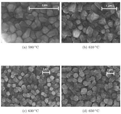
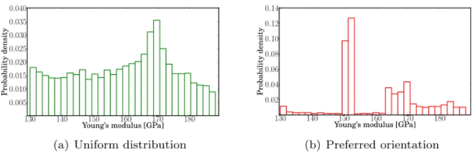
samples to define the uncertainties of the micro-structure. These measurements were provided by the IMT institute in Bucharest in the frame of an MNT ERA-NET project. The micro-structure being made of an anisotropic poly-crystalline material, i.e. poly-silicon, the randomness in the grain size distribution and in their orientation –with or without preferred orientations– induce uncertainties. The grain size distribution is studied for different manufacturing temperatures by Low Pressure Vapour Chemical Deposition (LPCVD) based on Scanning Electron Microscope (SEM) images while the distribution of orientations, when considered, is obtained using X-Ray Diffraction (XRD) measurements. Another source of scatter is the surface profile of the MEMS structure as its roughness is of comparable size to the structure thickness in case of a thin device. The sur-face topology, when considered, is obtained thanks to Atomic Force Microscopy (AFM) measurements. Both the roughness and the grain structure are corre-lated as it is noted in [105].

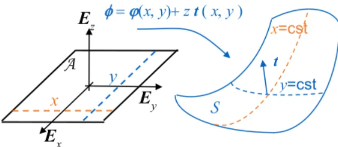
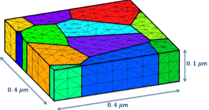
To achieve the second step of the method, i.e the homogenisation of the micro-structure over a volume element, the choice of the method depends on the macro-scale problem of interest. In this work, three cases will be considered. First order computational homogenisation, as described in [43], is used to study the mechanical material behaviour of the volume element. As we are interested in poly-silicon structures, the anisotropy of the grain crystal induces material uncertainties through the randomness of their orientation. These meso-scale uncertainties can be captured with first-order computational homogenisation. If the thermo-elastic damping is of interest at the macro-scale, the homogeni-sation procedure will consider the thermo-mechanical coupling as described in [48]. If uncertainties of the geometry, such as roughness, are to be taken into account, second-order gradient-enhanced homogenisation procedures are carried out on Rough Statistical Volume Elements (RSVEs) which would consider the material profile uncertainties. With a view toward macro-scale plate simula-tions, second-order homogenisation allows capturing the roughness effect on the bending behaviour of the meso-scale volume element as it provides a bridge not only between the in-plane stress and the in-plane strain, but also between the higher-order stress –i.e. bending moment– and the higher-order strain – i.e. curvature– as illustrated in Fig. 1.3. Second-order homogenisation was described for small strains in [37], and for finite strains in [45]. The method was adapted for shells in [10] or again in [11], where the method was applied to study the buckling of heterogeneous shells. Owing to the computational homogenisa-tion process, the stochastic meso-scale informahomogenisa-tion, i.e. the elasticity tensor or the shell-like resultant membrane, bending, and coupled material tensors, see Fig. 1.3, are then gathered following a simple Monte-Carlo scheme applied on (R)SVEs realisations.

Although by performing homogenisation on several (R)SVE realisations the marginal distribution of the different homogenised properties can be obtained, in order to propagate the uncertainties to the macro-scale, the spatial correlation has also to be evaluated. To obtain the spatial correlation between neighbouring (R)SVEs, a moving-window technique [5] is used on a sufficiently large material sample, thus estimating a discrete correlation function of the (R)SVEs

(21)

A 𝑆𝐹 𝑆𝐿 ℎ /2 𝑆𝑇 𝐷 𝑥 𝜺𝑀, Δ𝜺𝑀 𝜿𝑀, Δ𝜿𝑀 𝒏𝑀, ℂ𝟏, ℂ𝟐 𝒎̃𝑀, ℂ𝟑, ℂ𝟒 𝑙macro Meso-scale BVP resolution 𝝎 𝑙meso 𝑙micro

Figure 1.3: Homogenisation-based multi-scale method with 2nd_-order

homogeni-sation for macro-scale Kirchhoff-Love plates.

ties. The cross-correlation between the different meso-scale properties is also computed. Indeed, as stated in [89], the influence of the cross-correlation be-tween the Young’s modulus and the Poisson ratio on the response variability is negligible in case of a static problem but this assumption is not valid when a dynamic problem is involved.

Once the stochastic behaviour of the meso-scale (R)SVEs is evaluated us-ing a sufficient number of realisations, a random field can be defined, which is the third step of the method. The two main approaches usually considered to build a random field are the Karhunen-Lo`eve expansion, which was used in the recent work [8] for example, and the spectral representation method which was developed in [83, 85]. The latter procedure allows computing the discrete spec-tral density from the discrete correlation function evaluated by the stochastic homogenisation by recourse to Fast Fourier Transforms and is therefore chosen in this work. The spectral representation generates Gaussian fields, but non-Gaussian fields can be retrieved through an appropriate mapping technique [74, 98, 13]. As the non-linear mapping from Gaussian to non-Gaussian changes the spectral density, an iterative procedure is required to obtained both the desired spectral density and non-Gaussian probability distribution. Moreover, in order to ensure the existence of the expectation of the norm of the inverse of the material tensors, a lower bound is introduced during the generation process [12].

With the possibility of generating random fields, the fourth step can be performed i.e. the uncertainties at the meso-scale are then propagated up to the macro-scale. On the one hand, a unique stochastic approach will be used at the macro-scale: the Monte-Carlo procedure. On the other hand, different macro-scale analyses will be performed so that different problems can be studied. The first problem studied is the uncertainty propagation of the elasticity

(22)

tensor in linear elasticity towards the scatter in a MEMS resonator resonance frequency, the quantity of interest in this case. For the sake of simplicity, beam elements are considered at the macro-scale. This problem is used to verify the 3-scale procedure as a reference solution can be estimated. The reference solu-tion is obtained using full direct numerical simulasolu-tions, i.e. for which the grains are meshed, in linear elasticity combined to a Monte-Carlo method, which al-lows the probability density function to be computed. This methodology is computationally expensive due to the number of degrees of freedom required to study one sample. Nevertheless, it is a convenient approach to show that the stochastic multi-scale approach yields the same marginal distribution of the quantity of interest as the direct approach. The advantage of the multi-scale strategy is the use of coarser finite elements at the structural-scale which re-duces the computational costs. In the context of the 3-scale method, different SVE sizes and different structural-scale finite element meshes are successively considered to demonstrate that by accounting for the spatial correlation of the meso-scale homogenised properties, correct predictions are obtained if the dis-tance between integration points of the finite-element mesh remains smaller than the mesoscopic correlation length.

The second studied problem consists in estimating the uncertainties of the quality factor, the quantity of interest in this case, of a micro-beam modelled with 3D finite elements. Modelling both the resonator and its clamp will be per-formed. The thermo-elastic quality factor for micro-resonators can be extracted by recourse to multi-physics finite elements which considers the influence of the homogenised elasticity tensors, conductivity tensors and thermal expansion tensors.

Finally, the last problem focuses on the influence of the roughness on the resonance frequency, the quantity of interest in this case, of thins plates. To propagate roughness uncertainties, a more general macro-scale approach than the use of beam elements is considered. To take into account most of the available information at the meso-scale, such as the resultant bending mate-rial tensor (obtained thanks to the second-order homogenisation procedure), Kirchhoff-Love plate elements are considered. In particular, the plate elements are formulated using a displacement-only discretization by recourse to a Dis-continuous Galerkin method [95, 68].

For each problem, the variability of the macro-scale quantity of interest can be captured using a Monte-Carlo (MC) procedure. However, compared to the direct MC simulations, the recourse to the meso-scale random field obtained from the stochastic homogenisation allows the use of coarser macro-scale finite elements, reducing the total computational cost. The MC approach is an accu-rate, straightforward, non-intrusive tool to study complicated systems even if it involves a high random dimensionality. It is commonly used in many applica-tions, such as in engineering or finance. The recourse to MC is here acceptable provided that it is coupled with the 3-scale approach.

To summarise, volume elements representing the uncertainty of the micro-structure are generated based on experimental measurements. An homogeni-sation procedure allows computing the stochastic behaviour of the meso-scale

(23)

SVE size Mean value of material property Quantity of interest Probability density Stochastic Homogenization SFEM

Grain-scale Meso-scale Structural-scale

Variance of material property

SVE size

Figure 1.4: The 3-scale procedure

properties. The resulting random field description of the meso-scale material properties can be used with stochastic finite element methods to predict the probabilistic behaviour at the structural-scale. With this multi-scale method the meso-scale random field is smooth and has a correlation length larger than when considering explicitly the grain discretization. Hence coarser meshes can be used in the framework of the stochastic finite-element methods, eventually reducing the computational cost. The procedure is illustrated in Fig. 1.4. This process will be applied in linear elasticity for 1D free-clamped beams, for thermo-elastic 3D beams, and for rough thin plates.

1.3 Contributions

Both multi-scale methods and uncertainty quantification procedures are well established in the scientific community nowadays. In this thesis dissertation, we investigate the integration of uncertainties in the frame of multi-scale anal-yses to propagate uncertainties from the microstructure up to the quantity of interest at the scale of the structure. In particular, we develop an original stochastic 3-scale methodology which is verified by direct MC simulations. This stochastic 3-scale approach has been developed in the context of (i) linear elastic-ity, (ii) linear thermo-elasticelastic-ity, (iii) second-order homogenisation combined to Kirchhoff-Love plate formulation. Also the uncertainties of the microstructure are defined based on experimental measurements on poly-silicon films performed by IMT-Bucharest.

We published the following papers:

• Vincent Lucas, Ling Wu, Maarten Arnst, Jean-Claude Golinval, St´ephane Paquay, Van Dung Nguyen, and Ludovic Noels. Prediction of macroscopic mechanical properties of a polycrystalline microbeam subjected to mate-rial uncertainties. In Proceedings of the 9th International Conference on Structural Dynamics, EURODYN 2014, pages 2691-2698, 2014.

(24)

• Vincent Lucas, J-C Golinval, St´ephane Paquay, V-D Nguyen, Ludovic Noels, and Ling Wu. A stochastic computational multiscale approach; ap-plication to MEMS resonators. Computer Methods in Applied Mechanics and Engineering, 294:141-167, 2015.

• Ling Wu, Vincent Lucas, Van-Dung Nguyen, Jean-Claude Golinval, St´eph-ane Paquay, and Ludovic Noels. A stochastic multi-scale approache for the modeling of thermo-elastic damping in micro-resonators. Computer Methods in Applied Mechanics and Engineering, under revision.

• Vincent Lucas, Jean-Claude Golinval, Rodica Voicu, M. Danila, Raluca M¨uller, M. Danila, Adrian Dinescu, Ludovic Noels, and Ling Wu. Prop-agation of material and surface profile uncertainties on MEMS micro-resonators using a stochastic second-order computational multi-scale 3 ap-proach. International Journal for Numerical Methods in Engineering, Sub-mitted.

1.4 Outline

This work is divided into the following chapters:

• Chapter 2, SFEM in the frame of macro-scale simulations, focuses on the use of stochastic finite elements methods to solve problems at the structural scale. First, uncertainty quantification procedures are intro-duced. Afterwards, the SFEM approach is described and applied on 3 problems: the first one deals with beam finite elements, the second one extends the problem to 3D thermo-elastic cases, and the last one tackles the problem of thin plates.

• Chapter 3, Meso-scale material characterisation by computational homogenisation, describes the homogenisation procedure considered to capture the micro-scale uncertainties at the meso-scale. At first, a re-view of homogenisation procedure is done. Afterwards, the computational homogenisation considered in this work is described for the 3 distinct problems (first order homogenisation in linear elasticity, extension to the thermo-elastic case, and second-order homogenisation in linear elasticity). • Chapter 4, Stochastic model of the meso-scale properties, focuses on the meso-scale random fields. First, random fields notions are intro-duced. Afterwards, the case of positive-definite matrix is investigated. Finally, the spectral representation method is considered. It is used to generate random fields based on the results computed in Chapter 3. The generated samples are the input of the SFEM approach in Chapter 2. The implementation of the random field generation and its extension to the non-Gaussian case are described.

(25)

• Chapter 5, Application to MEMS, deals with the application of the procedure on MEMS micro-beams. First, modelling the micro-structure based on measurements is considered. Afterwards, the meso-scale ho-mogenised properties are extracted using the methods described in Chap-ter 3. Finally, the random fields are generated using the process described in Chapter 4 and used as input for the SFEM described in Chapter 2 to study the variability of the response of structures. This 3-scale procedure is applied for 3 cases. The first one, based on beam finite elements, is used to verify the procedure. A direct monte-carlo approach is considered to estimate the reference solution. The second problem considers the uncer-tainties in the thermo-elastic damping of MEMS micro-beam. Finally, the third problem focuses on rough thin plates and their variability in terms of resonance frequency.

• Chapter 6, Conclusions and perspectives, conclude the dissertation and present the perspectives.

(26)

(27)

Chapter 2

SFEM in the frame of

macro-scale simulations

The problem of uncertainty quantification is first investigated in the opening of this chapter. Afterwards, the stochastic finite element approach is introduced in Section 2.2. It is applied for 3 different problems in the last 3 sections of this chapter: beam elements in linear elasticity, the extension to 3D thermo-elastic problems and the case of Kirchhoff-Love plates.

2.1 Uncertainty Quantification

Nowadays, there is no need to defend the use of numerical simulations. At any design phase of a product, the recourse to numerical analyses is a very useful tool for the engineers. Often, numerical simulations allow engineers to avoid costly experiments. Deterministic models are mainly considered in in-dustrial applications. Sometimes, the model is such that uncertainties can be neglected. Sometimes, it is not the case and an uncertainty quantification pro-cedure should be considered. As described in [47], uncertainties can be classified in 3 categories:

• Model errors: when performing simulations, a mathematical model is used to represent reality. The assumptions considered to describe a physical phenomenon induce unavoidable uncertainties. For example, the motion of a spacecraft around the earth can be simulated based on a 2-body mathematical model with perturbation forces. This does not exactly represent reality, nevertheless the results are very useful. Modelling errors are thus an unavoidable sources of uncertainties and the error resulting from the assumptions behind the mathematical model should be rigor-ously assessed.

(28)

• Numerical errors: when a mathematical model can not be solved an-alytically, numerical approaches are considered. However, the recourse to numerical approaches inherently implies uncertainties, due to discretiza-tion steps, iterative algorithms, finite number representadiscretiza-tion for a com-puter, ... When performing numerical analyses, uncertainties are unavoid-able and should be lowered at most. However, there is always a trade-off between accuracy and computational efficiency (in terms of memory us-age, CPU time, ...).

• Data errors: a mathematical model needs parameters and data to represent the physical characteristics of the system of interest. Such pa-rameters, i.e. the geometry, material properties or external forces, are sometimes deterministic and sometimes subjected to variability. These variabilities can take many forms. The uncertainty of some parameters can be inherently random. For example, this is the case for environmental effects (wind,...). This is also the case when the manufacturing process of a system involve a scattering based on design tolerance. The variabil-ities can come from an uncertain knowledge of some parameters, such as uncertain experimental measurements. Finally, the variabilities can also be present during the early design phase of a system: some parameters of the design may not yet be fixed and are subjected to uncertainty. Such uncertainties, unavoidable when present, cannot be reduced but they can be considered and modelled.

The focus of this work concerns this last source of uncertainty. Due to the fabrication process of MEMS and due to the intrinsic uncertainty involved in poly-crystalline anisotropic materials, macro-scale quantities of interest are sub-jected to scatter. This scatter can be studied at an early-design phase following an appropriate uncertainty modelling strategy. It is assumed that data errors are the most important source of variability and therefore the two other sources of uncertainties are not modelled.

The modelling of uncertainty can be done in many different ways. In the case of interval analysis, only extreme values of uncertain inputs are considered and represented with interval numbers which possess their own algebra. The interval analysis can be used to study uncertain structural systems, e.g. [77] or [78].

The fuzzy logic, first introduced by Zadeh [103], can be seen as an exten-sion of the interval analysis where a membership function is considered for each interval. This fuzziness represents how much the uncertain property is in one interval. While in interval analyses the membership with respect to an interval was a Boolean value (either it is in the interval or it is not), it is a real value between 0 and 1 in the fuzzy logic. This logic, often seen in linguistic applica-tions, can be used in engineering numerical analysis. As an example, Fuzzy sets are used in [61] to study a dynamical system subjected to fuzzy uncertainties.

(29)

Even though interval analyses or fuzzy logic are possible ways to treat un-certainty, the recourse to the probabilistic formalism is much more common in the literature. While the membership function of a fuzzy set defines how much a variable is in an interval, a probability defines how likely the variable is in an interval. Probabilities can be associated to discrete and continuous quantities. In the continuous case, a probability density function is assigned to the random-ness. The domain of definition of the randomness is divided into infinitesimal intervals. The probability density function provides the probability associated to each interval.

The evidence theory, also named Dempster-Shafer theory (DST) can be seen as an extension of the probability theory where the probability is bounded with a belief (lower bound) and a plausibility (upper bound). The evidence theory can be used to study epistemic uncertainty (uncertainty due to a lack of knowledge). Finally, Bayesian statistics can be used to draw a priori estimation enhanced afterwards with new information. Such an approach, based on Bayes theorem which states the conditional probability of an event, can lead to efficient un-certainty analyses when only few samples are available. As no hypotheses are required a priori, it is useful in data mining. When the number of samples is high, the results are similar to those obtained with the probabilistic formalism. However, the Bayesian approach is computationally more expensive. Thus it is not a convenient approach when samples can be easily obtained.

The approach mostly encountered in the literature is the probabilistic for-malism and it will be used in this work. It is a convenient way to deal with uncertainties and a lot a tools are available in the frame of the probabilistic approach, which is not the case of evidence theory for example. Furthermore, regarding data availability, as we are dealing with numerical observations, we can compute enough samples to obtain convergence.

In the probabilistic approach, one can first define a probability space (Ω,_{T , P )} where:

• Ω is the sample space, which contains all possible outcomes of a random physical or virtual experiment;

• T is the event space, which contains all possible subsets of Ω;

• P is the probability measure, each event possessing a probability which defines its likelihood.

The probability measure P is defined so that the Kolmogorov axioms are satisfied. These 3 axioms are the following. The first axiom states that the probability P is a non-negative real number. The second axiom can be written as: P (Ω) = 1. Thus the probability of the whole sample space is defined. It can be seen as a normalisation condition. The third axiom states that, for any events_{B and C, if B ∩ C = ∅, then P (B ∪ C) = p(B) + p(C).}

A random quantity, defined over a continuous space R, can be modelled with a random variable X with a probability density function fu, referred to as PDF,

(30)

P (a 6 u 6 b) = Z b

a

fu(u) du . (2.1)

From the Kolmogorov second axiom, the probability density function of u defined over the space Ω satisfiesR_Ωfu(u) du = 1.

The cumulative distribution function, or CDF, noted Fu(u)∈ [0, 1], is

de-fined as:

Fu(u) =

Z u

−∞

fu(v) dv . (2.2)

The PDF (or the CDF) contains all the information about an independent random variable. However, it is convenient to define scalar parameters to ease the representation of a random variable. Let us introduce a function g of the random variable u. Therefore the expectation operator E over g(u) is established following:

E [g(u)] = Z ∞

−∞

g(u)fu(u) du . (2.3)

The mean ¯u is obtained for g (u) = u. It is a measure of the central ten-dency of the random variable. It is also the first moment of u. The moments are obtained by considering g (u) = un _{where n is the moment’s order. Central}

mo-ments are defined by considering g (u) = (u_{− E [u])}n. The first central moment is 0. The second central moments is the variance V [u]. The standard deviation σ is defined as σu=

p

V [u]. It is a measure of the dispersion of the distribution about the mean value. A convenient way to represent this dispersion is the co-efficient of variation, or COV. It is expressed in percent as COV (u) = σu

¯ u · 100.

The skewness, based on the third central moment, is a measure of the asym-metry of the distribution. A distribution with a positive (negative) skewness possesses a longer right (left) tail while most of the density of the distribution is concentrated on its left (right) side. The skewness γ1 of u is γ1u=

E[(u−E[u])3_]

σ3

u .

The fourth central moment is the basis of the kurtosis. The kurtosis is defined as: β_2u= E[(u−E[u])

4_]

σ4

u . It is a measure of the ”peakedness” of the distribution. A random variable can follow any distribution function (as long as the latter is normalised). In practice however, it is common to consider parametrised den-sity functions. Classified in different families, these denden-sity functions are fully characterised by a finite number of parameters. Among all the parametrised density functions, the most famous one is undoubtedly the Gaussian distribu-tion, also known as normal distribution. The Gaussian distribution relies on 2 parameters, the mean ¯u and the standard deviation σu, and follows the

proba-bility density function (2.4). fu(u) = 1 σu √ 2πe (u− ¯u)2 2σ2_u _. _(2.4)

(31)

Although most uncertainties that engineers are dealing with are not Gaus-sian, the Gaussian assumption is still often used. To understand the hegemony of the Gaussian distribution, two concepts must be introduced: the central limit theorem (CLT) and the maximum entropy principle (maxEnt).

In its general form, the central limit theorem states that the sum of a suf-ficiently high number of terms, each term being independent and identically distributed with a well-defined mean and variance, follow a Gaussian distribu-tion. The extension to non-identically distributed terms can be made under certain conditions. Thus a Gaussian distribution naturally occurs.

The maximum entropy can be briefly described in the following way. Based on Shannon entropy, the entropy of a random variable can be defined based on its probability density function. The higher the entropy, the higher the uncertainty on the random variables. This can be used to estimate a probability distribution with the maximum entropy principle. The latter states that, to avoid introducing bias and unknown information, the PDF to consider is the one maximising entropy as what is not known is uncertain. The PDF will be evaluated using all the information available and only the information available. When the only available information is the mean and the variance (e.g. few experimental samples), the Gaussian distribution is once again obtained. The maximum entropy principle will be described in Section 4.2.1.

Finally, many tools are available to deal with Gaussian distributions. Thus, these facts explain the recurrence of the Gaussian assumption.

As many engineering applications involve non-Gaussian distributions (e.g. Young’s modulus, which is by definition a strictly positive value), a mapping from Gaussian samples towards a non-Gaussian set of realisations is commonly used. A set of samples u following a distribution fu can be mapped to another

known distribution fv according to:

v = F_v−1(Fu(u)) , (2.5)

where v are the mapped samples following the distribution fv.

A system can involve more than one random variable. The joint proba-bility density function is an extension to higher dimensions of the PDFs, the joint probability density function being defined in an analogous way to the uni-variate case. In the context of a multivariate random space, a 1D prob-ability density function for one random variable can still be defined through the marginal distribution (without reference to the value of other variables) or through the conditional distribution (the other variables are considered to be known). In the remaining of this work, marginal probability density functions are considered if not stressed otherwise.

Two random variables u and v are independent if their joint probability respects:

P (u_{∪ v) = P (u)P (v) .} (2.6)

If u and v do not respect Eq. (2.6), u and v are dependent, correlated. If two random variables u and v are correlated (e.g., the age and weight of a

(32)

human being are correlated), one realisation of u depends on the corresponding realisation of v. The correlation is a measure of such dependency. Even though many ways to measure dependency exist, the most common way to compute the correlation is to study the linear relationship between the two variables (Pearson correlation). From now on, the correlation will refer to the measure of the linear link between the random variables through the covariance. The covariance R is a measure of their cumulative deviation with respect to their means:

Rv_u_{= E [(u}_{− ¯u) (v − ¯v)] .} (2.7) The correlation is the covariance scaled by the standard deviation of both random variables. Its values can range from [_{−1, 1]. It can be defined as in Eq.} (2.8) where Rv_u represents the correlation.

Rv_u= R

v u

σuσv

. (2.8)

Let us stress the fact that only the linear correlation is estimated in this case. Therefore, while two independent variables show a correlation of 0, two variables with a zero (linear) correlation are not necessarily independent. For example, if u defines uniformly distributed variables in the range [a, b], the linear correlation of v defined as v = u2_{is 0. Let us note that, in the case of normal distributions,}

a zero linear correlation implies independence. One should also keep in mind that correlation does not necessarily imply causation. Relationships can be coincidental or a third factor can be present, and therefore correlated variables should be treated with care. For example the number of firemen requested for fire fighting is correlated with the amount of damage. This does not mean less firemen should be called1_{. Furthermore, since mid 20th century, the CO}

2 level

in the atmosphere, the usage of computer resources and obesity all increased and are correlated2_{. It does not mean there is a true link between them.}

Dependency between variables can happen, dependency between the same variables located at different spatial position exists too. This correlation is referred to as spatial correlation and it is the key ingredient behind a random field. The same can be said with time and a random process.

A random process a (t) consists of a set of realisations of a at different time t. It can be continuous with respect to t (and thus the set of realisations is infinite) or discrete. A random process is said to be stationary if its stochastic behaviour does not depend on the time t. In other words, the correlation between two variables of the process only depends on their time interval δt and not on the absolute time t. As an example, stock market can be modelled with random processes.

A random field can be seen as an extension of a random process, defined over time, to a randomness defined over any manifold of dimension n. Let us focus on random fields defined over the 3D spatial space. Such a random field, denoted a (x), consists of a set of realisations of a over a domain of interest D

1

www.stat.ncsu.edu/people/reiland/courses/st350/correl.ppt

(33)

spaced by x. The random field can be continuous if the random variables are continuously distributed over the domain or discrete if a finite set of variables are defined over the domain. The spatial domain can be of any dimensions. In simple words, random fields are generally considered to stress the fact that the scatter between nearby values is smaller than the scatter between variables further apart. The random field is said homogeneous if its properties do not depend on the spatial position. In other words, one can write for a homogeneous field:

fa(x)(a (x)) = fa(0)(a (0)) ∀x ∈ D . (2.9)

The spatial correlation is defined as the correlation between the same random variable at different spatial positions. It can be defined as:

R (x, y) = E [(a (x)− ¯a) (a (y) − ¯a)] σ2

a

. (2.10)

In the case of a homogeneous random field, it solely depends on the spatial distance between the random variables τ , R (x, y) = R (x_{− y) = R (τ ). Let} us note that τ is a vector, the direction being of interest for a homogeneous random field. It is not the case any more for an isotropic homogeneous random field. If the field is isotropic, the stochastic behaviour of the field is the same in any direction. Therefore, the correlation solely depends on the scalar norm of τ , R (x, y) = R (_{||τ ||).}

The correlation length is a measure of the spatial correlation of a field. For a homogeneous field, it can be defined by [84]:

lC=

R∞

−∞R(τ )dτ

R(0) . (2.11)

Many examples of random fields exist. The landscape can be seen as a random field over the spatial domain. The ocean, whose height variations are time dependent, can be seen as a random field defined over both the spatial domain and the time t. An extensive review concerning random fields can be found in [94]. More consideration concerning random fields can be found in Chapter 4.

This section introduced uncertainty quantification, or UQ. Using UQ in an engineering simulation analysis involves three main steps.

• Assessing: the input uncertainty, its stochastic behaviour, has to be eval-uated. This involves PDFs, spatial correlations and cross-correlations. This can be achieved by numerical simulations, experiments, or measure-ments. Assessing the stochastic behaviour of homogenised material prop-erties using numerical simulations is the focus of Chapter 3.

• Modelling: a stochastic model encompassing the assessed stochastic be-haviour has to be developed. Often, this involves random fields. A stochas-tic model of the homogenised properties has to be built which would allow

(34)

generating random fields of those properties. The problem can be tackled in many ways and the use of a spectral generator combined to a non-Gaussian mapping is the focus of Chapter 4.

• Computing: once a stochastic model of the random inputs is defined, the uncertainty of the system response can be computed. The Stochastic Finite Element Method is a common way to compute the stochastic re-sponse using the generated random fields as input and is the topic of this chapter.

2.2 SFEM overview

The propagation of uncertainties towards a stochastic response (e.g. resonance frequencies or quality factors) of a system is mainly carried out today with the help of SFEM approaches [88],[24],[47]. SFEM stands for stochastic finite el-ement method and consists of an extension of the deterministic finite elel-ement framework for stochastic problems, both in statics and in dynamics. By using finite elements whose properties are random, SFEM can propagate the uncer-tainties through the mechanical system and evaluate its stochastic response. To analyse an uncertain system, the very first thing to consider is the repre-sentation of the stochastic uncertainties. In this work, the stochastic input is represented by a continuous random field defined over the domain of interest D. The generation of this random field will be carried out in Chapter 4, based on samples computed in Chapter 3. For now on, the procedure being generic, let us assume that all the stochastic input, which corresponds to the material parameters at each point of interest of the FE model, are gathered in a vector_U. This vector is defined for each spatial position x of the domain of interest D. It is thus a field and each realisation of the field is based on the multidimensional random vector θ3_{. Thus the continuous random vector field}

U (x, θ) is defined. The use of this field towards the evaluation of a stochastic response of interest, with the help of SFEM, involves three basic steps, as recalled in [88].

• Discretization of the stochastic fields representing the uncertain system properties,

• the formulation of the stochastic matrix, • response variability calculation.

2.2.1 Discretization of the stochastic fields

The discretization step is the approximation of the continuous random field U (x, θ) by a discrete field involving a finite number of random variables ˆU (x, θ). The discretization methods can be classified into three categories [48],[88]:

3_{In the remaining sections of this work, a variable depending on θ is random based, the}

ran-dom space being uni-dimensional. A variable depending on θ is also subjected to ranran-domness, the random space being multidimensional.

(35)

• point discretization methods where the continuous random field is modelled by its values at some given points;

• average-type discretization methods where the continuous random field is represented by weighted integrals over specified domains;

• series expansion methods where the continuous random field is mod-elled by a truncated series whose spatial functions are deterministic and its random space is defined by a finite set of variables.

The point discretisation method is often used due to its simplicity. Further-more, the distribution of the discretised field is the same as the distribution of the continuous field. The choice of the points of interest still needs to be carried out. Many possibilities exist such as considering the middle point of the finite elements, the nodal points, the integration points, the interpolation methods, or the optimal linear estimation. As shown in [14], the midpoint discretization method tends to over-represent the uncertainties in each element. The mid-point discretization method is easy to implement but its accuracy depends on the mesh discretization: the mesh elements must be small enough compared to the correlation length so that the properties can be considered constant over the mesh elements [48].

While the uncertainties tend to be overestimated with the midpoint dis-cretisation approaches, they are underestimated in the case of average-type discretisations [14]. Among the average discretisations, the local approach is the simplest one. The local average method approximates the random values associated to a mesh element as a constant which is the average of the original field over the element. It can be written as:

ˆ Ui(θ) = R DiU (x, θ) dx R Didx , (2.12)

where the domain of interest D is discretised with a finite set of mesh elements Di and ˆUi(θ) is the random vector associated to the finite element Di. Note

that there exist other average discretisation procedures such as the weighted integral method.

Series expansion methods can be written in a general way as:

ˆ U (x, θ) = N X i=1 αi(θ) φi(x) , (2.13)

where φi(x) are deterministic spatial functions and the αi(θ) are parameters

representing the randomness. The point discretisation and the local average methods can be seen as particular cases of the series expansion method. Spec-tral expansion methods can be based on the Karhunen-Lo`eve decomposition, polynomial chaos expansion or on a spectral decomposition. The recourse to spectral decomposition can lead to a reduction of the random space [48].

Let us note that the random field mesh is not necessarily the same as the finite element mesh, even though it is often the case as it eases the problem.

(36)

Actually, the accuracy of the discretisation of both meshes are based on different criteria. The discretisation of the random field is linked to the correlation length while the finite element mesh is based on the geometry of the structure or on the stress gradients. In some cases, it may be advantageous to consider different meshes. For example, if the random field is highly correlated (compared to the mesh size of the required finite element mesh), the stochastic mesh can be coarser to its corresponding finite element mesh so that the random space is reduced.

2.2.2 The formulation of the stochastic matrix

The aim of this section is to integrate the discretised stochastic fields defined in Section 2.2.1 in the finite element framework. This first requires to set up the deterministic problem. For example, for a static problem, the system of equations can be written as:

Ku = f , (2.14)

where K is the stiffness matrix, u the displacement, and f the external forces. Afterwards, the randomness can be added. In this example, uncertainties can come from the material and thus will be reflected on K or from random external loading, thus involving f , or both. If the stochastic response of a static structure experiencing random external loading through wind load is sought, the problem becomes:

Ku = f (θ) . (2.15)

In the frame of non-intrusive procedures, the stochastic problem is fully for-mulated at this stage. Non-intrusive procedures compute the stochastic response of the structure based on a set of samples of the response of the deterministic problem with random inputs. Non-intrusive procedures are convenient as the deterministic solver underlying the problem can be used as a black box.

2.2.3 Response variability calculation

Once the stochastic problem is defined, the variability of its response can be estimated. The most common way to deal with the response variability cal-culation is the Monte-Carlo (MC) simulation. Other methods exist, such as the perturbation approach or the spectral stochastic finite element approach (SSFEM).

The Monte-Carlo simulation is a straight-forward non-intrusive approach which is very often used due to its simplicity and accuracy. From one realisation of the stochastic input, one sample of the structure response can be extracted based on a deterministic approach. From a set of realisations, the variability of the stochastic response of the structure can be estimated with statistical tools. To achieve a given accuracy, the system must be solved a sufficient number of times. This method is accurate as long as enough samples are computed (law