Estimation of the size of informal economy in Russian Federation based on household budget survey data

(1)

HAL Id: dumas-01095923

https://dumas.ccsd.cnrs.fr/dumas-01095923

Submitted on 16 Dec 2014

HAL is a multi-disciplinary open access

archive for the deposit and dissemination of sci-entific research documents, whether they are pub-lished or not. The documents may come from teaching and research institutions in France or abroad, or from public or private research centers.

L’archive ouverte pluridisciplinaire HAL, est destinée au dépôt et à la diffusion de documents scientifiques de niveau recherche, publiés ou non, émanant des établissements d’enseignement et de recherche français ou étrangers, des laboratoires publics ou privés.

Estimation of the size of informal economy in Russian

Federation based on household budget survey data

Yaroslav Murashov

To cite this version:

Yaroslav Murashov. Estimation of the size of informal economy in Russian Federation based on household budget survey data. Economics and Finance. 2014. �dumas-01095923�

(2)

Université Paris1 – UFR 02 Sciences Economiques

Master 2 Recherche Economie Théorique et Empirique

"Estimation of the size of informal economy in Russian

Federation based on household budget survey data"

Nom du directeur de la soutenance: Francois Gardes

Présenté et soutenu par : Murashov Yaroslav

(3)

2

L’université de Paris 1 Panthéon Sorbonne n’entend donner aucune approbation,

ni désapprobation aux opinions émises dans ce mémoire ; elles doivent être

(4)

3

The definition and methods to identify the informal economy.

Black economy is by definition the activity concealed from law. So it will not be indicated in the official revenue documents. Although, if we are looking at the revenue surveys, they may include some information about the black economy activities, but to some extent, because people still have some incentives to conceal black economy activities. Therefore, researches may try to estimate the part of the economic activity which is treated as the black economy. One of the ways to estimate the black economy is microeconomic approach and is based on the data obtained from households budget surveys. The key idea is that the households indicate their expenditures more accurately than they indicate their income.

Actually, the main idea of the authors Pissarides and Weber, 1989 [3] is that 1) the reporting of expenditure on some items by all groups of population is accurate; 2) the reporting of income by some groups of the population is accurate;. Actually, the income reporting is accurate not by some groups, but by some types of occupation of the population. The authors believe that the expenditure item which is recorded correctly is the expenditures on food (the less likely to conceal). The underreport of income comes from the people who are self employed. Employees report their income correctly. Although this may look like a strong assumption that only the self - employed are those who under - report their income, because for most of the people to indicate the wage expenditures is not always reasonable. They may obtain other wages which are not indicated in the responses to the questionnaire. That is why it may be important to use the variable of total income earned by the household, which is not divided into subgroups and may be used as the base for calculation of self - employment income.

Therefore, the authors propose straightforward method to estimate the size of black economy. First, an expenditure function is needed to be calculated. Then the expenditure function is inverted and the income is forecasted from the reported expenditure.

First of all it is important to build a theoretical model, describing household consumption patterns, to account for the underreport of income on the one hand, and the connection between income and consumption, on the other hand.

The variables reported by the households: 1) consumption of individual items ( is the

household index, is the index of the index of the consumption item); 2) after - tax income ; 3) vector of household characteristics . According to our assumptions, there is underreport of the level of income for households in self - employment. Denote by the coefficient by which a household is underreporting their income. Then the connection between the factual and reported income is written in the following form: . So for employees and for the self - employed. The expenditure function of item is written in the following form: . It is needed to note the definition of . We denote by this the measurement of the income influencing consumption decisions. The relation between the permanent and actual income is measured by . This parameter accounts for the variation of income due to the unforeseen circumstances. The mean of does not depend on the type of the household and is the same for the employees and the self - employed. On the other hand, the variation of the parameter is different depending on the type of a household: . If the household is self - employed, then the variation of this parameter is higher, reflecting the higher variation of the self - employed income. That is why current consumption is a function of not a current income, but the permanent income.

(6)

5

Therefore, permanent income, which is directly related to the consumption function, can be decomposed into current income and the parameters of the model through the following way:

This implies existence of the two additional random regressors in the model if we put into the model observed income instead of the permanent income. To verify statistical hypothesis the authors must make assumptions concerning the statistical distribution of the coefficients responsible for the income mismatch. The coefficients have log-normal distribution. So now write them in the form of deviations from their means. ; . Now the trick performing the connection between the mean of and the mean of its log:

. As far as the mean of does not depend on the type of the household, one may compare the mean of the log for the employees and the self - employed: . How one can use this fact? Let us put the error terms decomposition into the expenditure function. Then we obtain the following decomposition of permanent income: . This decomposition can be used for the expenditure function. Then:

The dependent variable is the household expenditures on some particular item. In authors model food expenditures will be considered. The idea of this quite simple model is to obtain income differences for the self - employed. If this equation is estimated separately for employees and self - employed then the intercepts differ as far as is not the same at each group. This constant term may give information on the size of black economy.

To estimate this relationship the following type of regression model was used:

Where is a dummy variable taking value "1" if the individual is self - employed, and zero if he is employee. This model can be straightforward estimated by the method of least squares, accounting for the heteroscedasticity of error term . But how can we exactly compute the level of income under - reporting with the help of this model?

According with the theoretical income decomposition for the expenditure function the coefficient must be equal to the term

. We can see that our hypothesis for the equal coefficient for both self - employed and employees holds. This enables us to perform the model. From our previous discussion ; whereas . Therefore .

The estimated coefficient equals:

.

The income decomposition enables us to perform the reduced - form regressions for income. Therefore the observable income can be decomposed in the following form:

Due to the income decomposition, we obtain that ; or equivalently: .

(7)

6

Important implication of this decomposition is as follows: for given value of , and

are negatively related.

From the estimated coefficient we have that . Then we have .

We get the lower bound for mean under - reporting if ; the upper bound of mean under - reporting is obtained when is minimized. Having the income variance decomposition and assuming that the error terms and are not correlated we can determine the bounds for the level of income under - reporting. They are as follows:

With the help of this decomposition the interval for the level of income under - reporting can be obtained, since we have estimated the model of expenditures and computed the income variations.

The estimating procedure for this is quite straightforward:

1) we pick some expenditure item and monitor the households expenditure on it (the expenditures on the item should be reported correctly);

2) denote the type of the household (either a self - employed or the employee), according with the source of the main income (classified as self - employed if the income from self - employment is not less than 25% of total income);

3) estimate the model in the following form: , the aim

is to estimate the marginal propensity to consume and the parameter ; 4) estimate the income variance depending on the type of the household;

5) compute the lower and upper bound of the level of income under - reporting, assuming zero covariance between the errors in the model.

In the article written by Lyssiotou and Pashardes [2] the authors actually use the method of Pissarides and Webber [3] proposed in 1989 to estimate single food expenditure equation. But the authors go further n the estimation proposing the two other methods of black economy estimation.

The basic way of developing the model of Pissarides and Webber used by the authors is to include in the analyses the demand for durable goods. By dividing the demand into the demand for durable and the demand for non-durable goods one may notice that the share of income a household spends on durable goods depends not only on the level of income, but on the income source. Therefore, self - employment income may indicate not only income under-report, but the preference heterogeneity: self - employed people may tend to spend more on expensive goods (consumption of durable goods), therefore they are spending too little on food and other non-durable goods.

Another reason why the self - employment income is not a good proxy for the utility is that it tends to be more volatile, therefore, it influences savings. Households spend less and earn more than employees to meet the precautionary savings.

The authors separate the preference structure so that the consumption is divided between durable and nondurable goods. The cost functions of consumption are defined:

(8)

7

, where denote the sub-cost functions. Using this function one can depict household expenditure on the good:

The budget share of good in the expenditures on nondurable goods:

The authors impose the unit cost of nondurables . It has a quadratic logarithmic form:

Using this function by differentiating one can obtain Hiksian shares of the demand denoted above. This can be parameterized with the following function:

Given the cost function we can see that the expression

is directly linked to the level

of income of a household through the indirect utility function, so authors make linear decomposition of this expression as a function of , where is the true household income. As the result Hiksian demand shares can be written as:

where the parameters are a function of Hiksian demand shares parameters, the price index is dropped, since the prices are fixed at the level . The label denotes a household, the label denotes a good in the consumer bundle. This is the theoretical foundation for the Engel curve, since the consumption share depends on income as a quadratic function. The quadratic form of the Engel curve means that since the income of a household increases it tends to spend more expenditure share on luxury goods and less expenditure share on necessities.

The advantage of this model is that there is no need to arbitrary impose the type of a household. This can be seen through the following income decomposition:

The share of income earned by a household from a certain income source is computed, this is denoted by . The total real income of a household equals .

Dividing both part of the equation by the observable income: ; therefore . This helps to rewrite the Engel curve equation:

i

1) The model is more complex than one considered by Pissarides and Weber, 1989. But it can be linked to the model of Weber if one can impose a certain threshold in the share of household's self - employment income:

is replaced by

equals zero for all

The equation for the commodity according to Pissarides, Weber looks like:

(9)

8

This equation is estimated for the category of goods for which the income is reported the most correctly. This category is food expenditures.

Actually in the article the following model is estimated, almost similar to Pissarides, Weber:

The problem is that the expenditure on the left - hand side is actually varies along with not only the total income, but with the type of the household. Thus reflecting the preference heterogeneity:

The single equation approach does not distinguish these effects, that is why it is limited. The system approach can cope with this difficulty and is performed by the authors.

2) Actually the first way to estimate the black economy complementary to the Pissarides, Webber approach is to use the nonparametric approach. There exists a nonlinear function which determines the Engel curve equation for the household of each type. The idea is to estimate the nonparametric regression for each type of the household (employee, self-employed) and to measure the distance between the expenditures through the nonlinear part of the model:

3) The third method used by the authors is the demand system approach. As have been mentioned above, this method enables to account for both heterogeneity of preferences and income under - report. As in Pissarides and Weber, households are assumed to have two sources of income: income from wage and income from self - employment. But there is no a certain discrete type of a household: in the model authors use budget shares of the household income. The income under-report parameter does not include preference heterogeneity, since the heterogeneity is represented by a term shifting the Engel curve. The demand system is based on the household expenditures shares for non - durable goods. The following good categories are considered: food, alcohol, clothing, personal goods, leisure goods, fuel. The equation to be estimated is written in the following form:

There are three major differences of this model in comparison with Pissarides and Webber, 1989:

1) The authors estimate a system of budget share equations (the good is denoted by ); 2) They use not the dummy variables indicating the role of household occupation, but the share of income obtained from a certain activity;

3) The parameter is no longer responsible for the level of income under-report, but stands for the preference heterogeneity.

Estimation of the size of informal economy in Turkey estimated by Aktuna Gunes A., Starzec C., Gardes F. [1] is based on the model proposed by Lyssiotou and Pashardes, 2004. But now the authors assume that a household has three forms of income: wage income, self - employment and other income. The other income seems to be reported correctly, while the other income components may be hidden. Due to the fact , for

(10)

9

. Another enlargement is that the preference heterogeneity term depends on the share of each part of the income (the heterogeneity is viewed in the form of difference in savings between different occupation groups and consumption patterns).

The estimated system of equations is actually the same. The difference is that the system is estimated by generalized method of moments and the household production activities are included in the system in the form of household consumption and household production. So the initial model is enlarged and includes the consumption of household goods and the income from their production evaluated by the market price.

However, estimating the size of informal economy in Russian Federation we are not able to compute the value of household production since we do not know the amount of time used on a certain activity (there is no such a question in the interview neither on the household nor on the individual level). But there is the information on the household production of the agricultural goods. The money income from the goods sold is actually included in the household total income. The information of goods consumed is added to the goods consumption data to form full expenditures. The value of the household goods produced is computed on the basis of the purchase prices indicated in the interview paid for a certain type of commodity. Therefore, it represents the market valuation of household production.

On the first stage it is possible to estimate a single food expenditure equation and to see whether an income decomposition and the black economy coefficient can be obtained. To say in advance, there are some problems concerning both the income decomposition and the estimation of this coefficient. Therefore, the more complicated econometrician estimation methods should be used.

RLMS database description

Russian Longitudinal Monitoring Survey is the only annual nongovernment monitoring of social - economic characteristics of the population of Russian Federation and the health conditions [4].

Monitoring represents a series of representative questions based on the multi - level probability multi-step territorial sample.

The key peculiarity of RLMS is the wide - spread base of socio - economic variables. The variables include the income and expenditure structure, material welfare, investment, occupation, migration, health conditions, structure of food consumption, education. RLMS is denoted by panel data, modern methodology, data comparability.

What is special about the survey?

- The methodology of the questionnaire enables world - wide comparisons;

- Thanks to RLMS for the first time the researches got access to the alternative to government statistics microdata on the base of national sample;

- The monitoring program contains some important characteristics which are not available in the government statistics. It is the only survey containing the initial information on

income of certain household members and the households as a whole

- RLMS is practically the only representative microeconomic survey in Russian Federation having a large panel component: the same households are interviewed during a long period of time; this increases the quality of forecast based on RLMS;

(11)

10

- RLMS contains a large block of valuating questions which add to the information about the change in Russian households life activity by the subjective assessment of changes in the country.

RLMS has been conducted during the two periods: the first period survey has been made from 1992 to 1993; the second - since 1994 till now. All the work for the monitoring including the sample design, has been made by the Russian research team supervised by Kozireva P. M. and Kosolapov M. S.

Starting from 2006 National Research University - Higher School of Economics is playing a key role in the project.

The model of sample The dynamic aspects of the analysis of changes in the households claims "panel" sample model, where in each wave the same household members or individuals are questioned. But with the time this panel sample is growing older, certain elements disappear and systematic bias arises. Therefore the panel model does not allow for a clear situation at the moment of the new wave. This task is accomplished by cross - sectional model of sample.

The cross-sectional data is combined with the panel. The model was chosen such that along with cross-sectional sample enables to provide panel analysis. This solution is named repeated sample with split - panel. The advantage of the repeated sample is that it provides data analyses on both the households and the household members.

The data collection periods of RLMS include 21 waves. The last one has been conducted from October 2012 to December 2012.

Our attention is devoted to the study of households of cross-sectional analyses - the households which represent the population of Russian Federation and actually live at the adresses included in the survey.

The identification variables are used to identify households and individuals in different waves. In each wave besides the identification variables of the same wave there are also identification variables of the preceding waves.

The first part of the research will be devoted to the analyses of representative sample for the household in the last wave of the research. The number of this wave is 21. The RLMS household budget survey has been conducted in this wave from October 2012 to December 2012. We have the representative sample which represents the population of Russian Federation at the moment the survey has been conducted. It means that only the individuals which are available at the place of their living are interviewed. That is why the sample represents the current situation in the household, and, as far as the sample is representative, the current situation in Russian Federation.

The wave contains the file of individual data and the file of household data. The file of individuals contains unique individual identification number for each respondent. Also it contains the number of household the member of which the individual is during the wave. This linked to the household number in the file of the household. As far as the unit of observation in our analyses is a household, this link from individual to household is used to merge the data from individual database with the data from the household database.

At the first stage, this database merging must be made. It is performed by sorting individuals by family number and by the variable of interest. Then the needed variable is kept and added to the household database. The following individual variables are used:

(12)

11

D_couple=1: an individual is in a registered marriage (we have a family) (_marst==2);

D_widow=1: an individual is a widow (_marst==5); D_divorced=1: an individual is divorced (_marst==4);

The basic group of a family status is lonely or not registered relationships. 2. Occupational status (if any member of a household has a given occupation):

D_white_collar=1: occupational status of an individual is one of the following - 1) law-makers or government workers (_occup==1), 2) specialists of higher qualification level (occup==2), 3) qualified agricultural workers (_occup==6), 4) qualified workers of hand - work (_occup==7), 5) other qualified workers (_occup==8). The basic group is blue collar workers, therefore blue collars are occupied in one of the following spheres: specialists of average qualification level, clerks, workers in the sphere of trade and service;

D_white_collar_male=1: occupational status of the head of the family is white collar (D_white_collar==1) & (D_male==1~h5==1);

3. Level of education (if any member of a household has a certain education degree): D_educ_sec_special=1 finished special education (_diplom==5);

D_educ_higher=1 finished higher education level (or higher) (_diplom==6); The basic educational group is the group of either full or not full secondary education.

4. The level of life satisfaction (if any member of a household reports that he is fully satisfied with life)

D_life_satisfaction=1 (j65==1);

5. The presence of some stomach deseases: D_stomach_desease=1 (m20_65==1). This variable may be useful when estimated household demand for food;

6. The desire to find another job: D_wish_other_job=1 (j81==1). This variable indicates whether the household may be willing to participate in informal economy activities;

7. The children in the household: D_children=1 (j72_171==1);

8. The number of children in the household: D_number_of_children (j72_172);

9. The ability of a household to improve the living conditions: D_living_improvement (j721631==1);

10. The ability of a household to have a vacation with all members of the family: D_vacation_possible (j721634==1);

11. The ability of a household to pay for a child study in the University: D_child_study_pay (j721635==1);

12. The presence of some other job at one member of the household: D_have_other_job (j32==1).

So what is the major difference between the characteristics of individuals in the households with no income from self - employment and those with high level of self - employment income? The comparison of individual characteristics of the households can be seen in the Table 1.

(13)

12

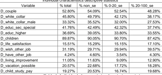
Individual characteristics descriptive statistics

Variable % total % non_se % 0-20_se % 20-100_se D_couple 52.80% 54.09% 52.54% 48.28% D_white_collar 45.80% 49.79% 42.12% 38.17% D_white_collar_male 33.32% 35.52% 32.00% 27.53% D_educ_sec_special 41.76% 42.49% 42.32% 37.74% D_educ_higher 36.69% 39.05% 33.80% 33.55% D_children 89.87% 90.05% 90.70% 87.42% D_life_satisfaction 15.51% 15.29% 15.15% 17.10% D_wish_other_job 31.19% 29.71% 29.94% 39.57% D_have_other_job 4.24% 4.60% 3.54% 4.30% D_living_improvement 11.05% 11.63% 9.09% 12.90% D_vacation_possible 20.57% 22.68% 17.72% 18.28% D_child_study_pay 19.27% 20.53% 16.74% 19.68%

Table 1. Individual characteristics descriptive statistics

Considering the family status self-employed are usually single than married. They are more involved in the non - qualified labor, both for the head and other members. They have lower level of education: both higher education (33.55% vs 39.05%) and secondary special education (37.74% vs 42.49%). They report a bit more higher level of life satisfaction (17.10% vs 15.29%). The greater part of them does wish other job (39.57% vs 29.71%). But they do not in general indicate that they have other job (maybe they conceal their shadow part of income, or simply do not have other job for which to be paid). To speak of financial possibilities, their possibilities to improve living conditions, have vacation, pay for child study do not differ from the average sample level and the level of non self-employed but exceed the possibilities of those who have minor share of self employment income. Therefore some of these characteristics may be very useful to account for the structural differences between different household types and used in regression analyses.

All these variables represent individual characteristics but are attributed to the households. They are used in the regression model to reflect the differences in preferences between the individuals. The choice of variables comes mainly from the database restrictions and the representation of key socio - economic characteristics. Also the variables include the questions giving information about the possibility of households to spend money on various activities.

The part of the survey devoted to the households also has the variables characterizing households but not the income or expenditure components.

These are the questions concerning:

1. The place of living: type of town, population.

2. Living conditions: type of house, price, home owner, total area, living area, number of rooms, central heating, central water, hot water, canalisation, telephone, magistral gas, electro owen, refrigerator, frost, auto washing machine, micro wave owen, dish washing machine, colour TV, TV plazma, videopleer, DVD_pleer, computer, notebook, low speed internet connection, digital camera, video camera, MP3 pleer, GPRS navigator, home auto, import auto, lorry, motor cycle, bicycle, tractor, lawn mower, air conditioner, sputnic antenna, cabel TV, garden house, other appartment.

3. Some variables concerning land use: have you got any land at use; the land area; has you paid for land; have you grown something, have you sold something.

(14)

13

4. The educational questions: do children go to school; does a household member visit college.

Here you can see (Table 2) the descriptive statistics of these variables with respect to income groups subsamples (the decomposition of income see at the income decomposition description section):

Condition Variable % total % non_se %

0-20_se % 20-100_se status==4 Village 24.0% 21.2% 24.8% 33.2% status==3 small town 5.6% 5.9% 5.2% 5.3% status==2 Town 26.3% 27.4% 27.7% 18.7% status==1 City 44.1% 45.4% 42.3% 42.8% Popul (mean) population 1541327 1590014 1468026 1504747

c1==1 your_house 88.9% 89.6% 91.3% 81.4% c1==2 D_rent_house 8.8% 8.6% 7.0% 13.3% c1==3 D_common_house 2.2% 1.7% 1.7% 5.3% c1_1 (mean) dwelling price 1923205 1973695 1856279 1866193

c4_0==1 self_owned 90.1% 91.0% 89.0% 89.0% c4_0==2 D_home_relative_owned 3.9% 3.6% 3.7% 5.3% c4_0==3 D_home_not_privatised 6.0% 5.4% 7.3% 5.7% c6 total_square 54.9 54.9 54 57.1 c5 living_square 36.7 36.4 35.8 39.5 c5_1 number of rooms 2.3 2.3 2.3 2.4 c7_1==1 D_cental_heating 71.7% 74.6% 70.4% 62.9% c7_2==1 D_central_water 87.8% 88.7% 87.0% 85.6% c7_3==1 D_hot_water 66.2% 68.5% 65.4% 58.7% c7_5==1 D_canalisation 73.7% 76.8% 72.3% 64.3% c7_6==1 D_phone 59.1% 59.3% 63.4% 49.2% c7_7==1 D_magistral_gas 66.0% 67.9% 65.5% 60.0% c7_8==1 D_owen 23.4% 24.2% 21.5% 24.3% c9_1_1a==1 D_refrigerator 49.5% 51.3% 46.8% 48.0% c9_2a==1 D_frost 11.9% 12.4% 11.1% 11.5% c9_3_2a==1 D_washing_machine 72.3% 74.9% 68.6% 69.9% c9_3_1a==1 D_micro_wave 61.2% 63.0% 58.9% 58.5% c9_3_3a==1 D_dish_washing 2.7% 3.1% 1.9% 3.0% c9_5_1a==1 D_colour_TV 78.5% 77.9% 81.2% 75.7% c9_5_2a==1 D_plazma 42.3% 44.7% 40.2% 37.3% c9_6a==1 D_pleer 24.7% 26.3% 23.2% 21.9% c9_6_0a==1 D_DVD 45.5% 45.1% 44.3% 49.0% c9_621a==1 D_computer 42.1% 44.6% 39.2% 38.5% c9_622a==1 D_notebook 32.3% 33.9% 28.1% 34.7% c9_623a==1 D_low_speed_int 18.1% 18.8% 16.3% 19.5% c9_624a==1 D_high_speed_int 37.0% 38.8% 34.2% 36.0% c9_6_3a==1 D_digital_camera 36.9% 38.8% 33.6% 36.5% c9_631a==1 D_video_camera 7.7% 7.8% 7.6% 7.4% c9_6_4a==1 D_MP3 10.4% 11.1% 8.8% 11.0% c9_6_5a==1 D_GPRS 7.2% 8.1% 6.1% 6.5% c9_7_2a==1 D_home_auto 22.0% 21.4% 23.2% 21.6% c9_7_3a==1 D_import_auto 20.7% 23.3% 17.3% 17.6%

(15)

14 c9_7_1a==1 D_lorry 2.3% 2.3% 2.0% 2.9% c9_8a==1 D_motor_cycle 3.1% 2.9% 3.2% 3.7% c9_8_1a==1 D_bicycle 21.2% 20.1% 23.2% 20.9% c9_9a==1 D_tractor 2.4% 2.1% 2.3% 3.7% c9_9_1a==1 D_lawn_mover 7.5% 8.0% 7.5% 5.2% c9_13a==1 D_air_conditioner 8.2% 8.1% 8.2% 8.3% c9_14a==1 D_sputnik_antenna 17.0% 15.5% 17.4% 21.9% c9_15a==1 D_cabel_TV 30.5% 32.4% 29.5% 25.1% c9_101a==1 D_garden_house 21.3% 22.6% 21.6% 15.3% c9_12a==1 D_other_appartment 8.5% 8.6% 7.9% 9.7% d1==1 D_land_use 50.1% 49.1% 52.2% 49.4% d5==1 D_paid_land_use 34.2% 34.0% 34.6% 34.2% d7==1 D_grown_smth 44.8% 43.4% 47.7% 44.2% d9==1 D_products_sold 2.1% 1.1% 2.2% 5.7% h21==1 D_secondary_education 30.4% 28.5% 30.6% 37.6% h45==1 D_college 16.8% 17.1% 14.7% 19.9%

Table 2. Descriptive statistics of household characteristics

Actually, there is quite little information to take from this descriptive statistics table. The percent values define the share of people in the sample which own a certain durable good or have a certain occupation. Most of the mean values of the variables do not differ from one occupational group to another. There can be made no conclusion that self - employed have a greater amount of durable goods and therefore that their wealth is higher. Maybe that is due to the fact that the ownership of these goods are not reported in the interview.

Despite this, some conclusions can be made from this table. The self - employed tend to be more settle in the village (33.2% vs 24.8% and 21.2% non_se), and also have more share of people which sell their products grown (5.7% vs 2.2% and 1.1% non_se). Less part of self - employed have phone (49.2% vs 63.4% and 59.3% non_se) Therefore, maybe some part of their income may be the agricultural income from the selling of products. Also as we have mentioned in the literature review the agricultural goods consumption shall be included is household foods product consumption to provide unbiased value of food consumption. This is the point to correct our model.

Income decomposition

An important part of our study is to see how income is decomposed between the different sources among the households. First of all, the total income of the household consists of three parts: 1) wage income free of taxes; 2) the part such as other income usually fixed income; 3) income from self-employment. The last one is actually computed as a difference between total income of a household, the wage income and the income from all other sources (which form non_wage income in our model, more precisely other income). So the formula by which the income is built is looking as follows:

(16)

15

The non_wage income of a household includes: pension; scholarship; unemployment benefit; income from equity sold; income from rent of equity; capital income in the form of the interest; capital income in the form of the dividend; insurance premium; aliments; money from the debt reimbursement; subsidies from the appartment payment. Actually the inclusion in this form the income from equity sold does not prove to be reasonable, because it is not a permanent source of income and therefore may be misleading. For the first time let us distinguish between non_wage income and other income. First is simply the difference between total income and wage income. While "other income" is free of self - employment income.

Now let us introduce some descriptive statistics to characterize the variables of interest. Here are the descriptive statistics of non_wage part of the income (Table 3). As you can see in the descriptive statistics, the most popular item indicated by the households is pension, indicated by 3910 households out of 6517 in the total sample. As an outlier stands the income from equity sold. There are quite few observations, but they account for the maximum value of one million and seven hundred thousand rubles. Therefore we do not include this form of income in the household sources of income.

Speaking about the income from capital (to the capital income we must denote the income from rent of equity, capital income in the form of interest and capital income in the form of dividend) we notice that there is very low rate of response (only 150 people have indicated that they have got income in some of the forms). This can be explain twofold: 1) most of respondents conceal the real amount of capital income because of the fact that they do not want to give any information about the total amount of capital owned; 2) the capital forms of income are not so popular in our country with comparison to the households in the western countries. Anyway, there is a reason not to believe these figures and consider that there is something behind them. We must say that non_wage income computed using the information on capital income is under - reported. Therefore, the self - employment income as it is defined must include some forms of capital income. So both parts: capital income which is fixed and less variable then self - employment income are under - reported and must be estimated. Although while the former is concealed, it is not mandatory that it is concealed for the reason of tax evasion and therefore should be viewed as a part of black economy.

(17)

16

Variable names

stats Pension scholarshi p unemployment benefit income from equity sold income from rent of equity N 3910 287 131 77 105 Mean 13786.81 1815.129 2996.412 139027.3 11952.38 Min 1030 300 400 500 2000 Max 64658 13000 80000 1700000 50000 p25 8500 600 1000 7000 4500 p50 11600 1200 2000 18000 9000 p75 17775 2000 3000 48000 15000 Variable names stats capital income in the form of interest capital income in the form of dividend insurance premium aliments money from the debt reimbursement subsidies from the apartment payment N 43 5 9 184 164 1592 Mean 6717.86 11320 23874.67 5820.625 6429.055 975.7469 Min 20 400 1800 300 50 50 Max 50000 40000 120000 35000 150000 6800 p25 1000 1200 7000 2500 1000 500.5 p50 2000 5000 10000 4000 2000 800 p75 7500 10000 20000 6600 5000 1200

Table 3. Indicated parts of non wage income

The sources of income which are combined under the name "other income" represent the following items: pension; scholarship; unemployment benefit; income from rent of equity; capital income in the form of the interest; capital income in the form of the dividend; insurance premium; aliments; money from the debt reimbursement; subsidies from the house payment. We exclude income from equity sold from the items including in "other income". The wage income, other income and total income provide the basis for the computing of self - employment income. "non_wage income" represents the difference between total income and wage income. The description of household income decomposition can be seen in Table 4.

Variable names

Stats wage_inc total_inc other_inc non_wage_inc self_employment_inc

N 4412 6215 4475 4844 3786 "zero" value 2105 302 2042 1673 2731 Mean 33699.99 36547.41 13477.98 16196.9 4792.341 Min 990 400 85 -375400 -381000 Max 420000 425300 175000 332300 320300 p25 15000 16000 7800 7614 100 p50 26000 27600 11200 12359 1448.5 p75 44000 45430 17800 20205 5917

(18)

17

As one can see from this table, positive total income is indicated by the most of households, only 302 do not indicate their income. For the analyses we do not distinguish between "zero" value of the variable and the "missing" value, since for the wage income those who report "zero wage" are added to those who report "I do not get any wage income". So a considerable part of the sample (2105) say they do not get any wage. These may be pensioners for whom pension is the only source of income.

Now we turn to the description of non_wage income: as we can see "zero" value of non_wage income is attributed to 1673 households. As far as this is simply the difference between total income and wage income, one may suppose that this is simply the amount of the households for which all the income is formed by wage. Another interesting characteristics of non wage income is that some have negative non_wage income, as well as self employment income. It means that for the households the total income is indicated incorrectly and it must be replaced by the sum of wage income and other income . We make the replacement for those households for which the value of non_wage income and income from self_employment is negative. It means automatically that self_employment income for those households becomes equal zero. But for a moment we will denote the households with the "wrong" self - employment income as a special part of a sample.

The corrected descriptive statistics table (Table 5) for the income decomposition looks as follows:

Variable names

Stats wage_inc total_inc other_inc non_wage_inc self_employment_inc

N 4412 6359 4475 5241 2880 "zero" value 2105 158 2042 1276 3637 Mean 33700 37126 13478 16676 9405 Sd 29838 33929 9532 18867 21905 sd/mean 0.89 0.91 0.71 1.13 2.33 Min 990 130 85 50 0 Max 420000 425600 175000 332300 320300 p25 15000 16200 7800 8000 990 p50 26000 28000 11200 12500 2724.5 p75 44000 46408 17800 20200 9000

Table 5. Descriptive statistics of income decomposition

Now in our sample the amount of "zeros" from non wage income diminishes thanks to the fact that for some households total income has been increased by the inclusion of other income. On the other hand, the amount of zeros from self-employment income increases thanks to the fact that we have substituted the negative values by zero values because of mismatch between total income and its components.

According to the descriptive statistics table, the mean value of wage income is the greatest among all the mean values of various income sources: households who get wage report that they earn on the average 33700 rubles, whereas the mean for other income accounts for 13478 rubles, self employment income is on average 9405 rubles, and one must take into account the fact that this mean is only above those, who happen to have positive amount of income (near 45 % of the households). So on average, the income from self - employment is much less than the wage income. It must be found whether it is true or not and what part of household income from self - employment is hidden.

(19)

18

Coming to the variations of different components of household income we must notice that the assumptions proposed by Weber are fulfilled: self - employment part of income is much more relative variant. What does it mean? Although the variance of wage income is more than the variance of income from self - employment, the relative variance, or the variance related to the mean, is much greater for those who are self - employed (2.33 vs 0.89). On the other hand, the relative variance of other income, which is defined above and consists of the sum of pensions, scholarships and so on, is the least (0.71).

That is why we are able to perform the income decomposition according to the idea, proposed by Weber: we believe that the wage income is reported correctly and the self - employment income is under - reported, that is why we need to compute the multiplier to perform the income correction up to the true level of self - employment income.

The next step of our model is to compute the part of total income which is associated to the self employment income. This will help to define the main part of household occupation. For those households who have self employment income one can perform a histogram of the income share distribution (condition if the share > 0) - Graph 1:

Graph 1. The density of self employment share of income distribution (self-employment income >0)

We can see that the distribution of the share of the self - employment income in the total income of household is skewed towards 1. It means that even if a household has some self - employment income, the majority of the households is still having it as a minor source of income.

The wage share distribution has an opposite skew in relation to the self employment income distribution. Have a look at the distribution of wage income share if it is either greater than 0 or less than 1 (Graph 2):

0 2 4 6 8 D e n si ty 0 .2 .4 .6 .8 1 self_employment_share

(20)

19

Graph 2. The density of wage share of income distribution (wage income share greater that 0 and less than 1)

The density of distribution increases with the two "steps" which occur at the share of 0.2 and 0.4.

Now we must determine the criteria, by which the household is self - employed. Following Webber, the criteria is such that the share of income from self-employment is greater than some threshold value. In our model this value is defined with the help of histogram of income share distribution. Let us say that this value is 0.2 (in the paper authors take the value of 0.25). 0 .5 1 1 .5 2 D e n si ty 0 .2 .4 .6 .8 1 wage_share

(21)

20

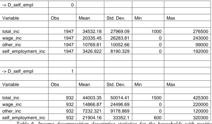
-> D_self_empl 0

Variable Obs Mean Std. Dev. Min Max

total_inc 1947 34532.18 27969.09 1000 276500 wage_inc 1947 20335.45 26283.81 0 243000 other_inc 1947 10769.81 10052.66 0 99000 self_employment_inc 1947 3426.922 8190.329 0 192000 -> D_self_empl 1

total_inc 932 44003.35 50014.41 1500 425300 wage_inc 932 14866.87 24496.69 0 220000 other_inc 932 7232.321 9178.869 0 120000 self_employment_inc 932 21904.16 33352.1 600 320300

Table 6. Income decomposition descriptive statistics for the households with positive income from self employment, grouped by the share of self employment income in total income

Here there are the descriptive statistics of income decomposition for households with self-employment income (Table 6). Households with high self-employment income have mean higher total income and slightly less mean other income. We have seen earlier that self-employment income has higher coefficient of relative volatility than wage income. Surprisingly this is not true for our types of households with positive income from self employment. Wage income tends to have the same volatility as income from self - employment, but even higher relative volatility for those who are self - employed. Although self employment income is more volatile in second group, the relative variance is smaller. But total income for self employed part of sample is anyway more volatile (in absolute and relative terms). To sum up, the hypothesis of income variance holds but only for the absolute income variance (except for the variance in wage income).

To perform the income decomposition proposed by Webber one must be sure that the total income and the income earned by the self employed are log - normal. The hypothesis of log-normality of total income cannot be rejected: Kolmogorov - Smirnov test has a P-value of 14.7%. Whereas for the self - employment income the statistics has a P-value of 1.4%, log - normality also can be assumed.

Concluding with the descriptive statistics analyses we must say that the income of Russian households does not necessarily come with the British households income behavior. Especially it can be seen that wages may be as much volatile as self - employment income. This fact says that maybe some new estimation methods should be implemented to estimate the size of black economy.

(22)

21

Expenditure decomposition

As far as we know from the theory, the household expenditure can be decomposed into the expenditure on durable and nondurable goods. Let us try to perform this decomposition with respect to our database. In RLMS the items of expenditures are grouped by the categories. This simplifies the analyses and enables to join the items by the same expenditure purpose. The items we are interested in are food expenditures, clothes expenditures, service expenditures (all of them form the expenditures on nondurable goods). The durable goods expenditures are also needed and include expenditures on household appliances.

To start with let us describe the food expenditures in our sample. The households are interviewed on the amount of food products purchased, their prices and total expenditures. This information is obtained for the last seven days. Actually our aim is to analyze the information on the household expenditures on food products and to aggregate it. The question is how can we use the pricing information, since we are operating with the aggregated items. The pricing information is not used at the moment. The household expenditures on food during the month is just the sum of expenditures on all products bought normalized to the 30 days period. Here you can see the table of descriptive statistics of consumer expenditures on each item sorted in the order of the highest mean value (Table 7 in the application). The mean value and variance are calculated for all sample. You can see that there is just a part of items on which you have positive numbers of amount of money spent.

It is interesting to look at the amount of food products indicated as consumed by the consumers. "Consumption" means that people indicate positive amount of money spend. The rate of response to this part of interview is almost 100%. So the zero consumption is due to the fact that people indicate they do not consume those types of products.

We have generated the variable responsible for the amount of items, for which consumers have positive expenditures. The distribution of the variable can be seen in the table for the three parts of sample: 1) the people with the share of self - employment income from zero to 20 percent; 2) the people with the share of self - employment income above 20 percent; 3) the people with zero share of income from self - employment. So the table says that the median amount of items consumed is only 15 out of 57. Is that quite little? This is sufficient to build and estimate the model: this is quite sufficient for a budget survey, and the amount of average expenditures on consumption correspond to reality.

The main idea of the Table 8 (see application) is to find out whether the rate of responses of households on the questions depends on the occupation status: is it true that those who have self employment income and tend to deliberately reduce their incomes have the same rate of response on the questions concerning food consumption as those who have only wage income or pension? We see that cumulative distribution function of the number of questions answered by those who have zero percent of income from self - employment and 0-20 percent go slightly behind the function of the people with high share of self - employment income. It means that a typical self - employed is saying he is consuming 1 product item less than the man living on wage income. Of course, this is a minor difference. We must accept the hypothesis that self - employed have the same pattern of food consumption as the other income groups.

On the basis of the summation of these expenditures one may obtain the value of total expenditures of a household on food products. That is simply the amount of goods purchased by a household during a week. But as far as there is the detailed representation of food goods purchases, there is also a question of the amount of the expenditures on food outdoors during the

(23)

22

last seven days. More than that, there is the question: "how much the households spent both on food at home and outdoors during the last thirty days". There can be traced the difference between our computed value as the sum of household expenditures on different items and the calculated value from the database on food expenditures at home.

Variable Obs Obs > 0 Mean

Std.

Dev. Min Max food_total_30 6517 6000 8784 7341 0 73000 food_outdoors_30 6517 2366 1550 3839 0 77143 food_at_home_30 6517 5743 7233 7198 -53143 61785 food_exp_purchase_30 6517 6498 9518 8297 0 181847 food_total_30_comp 6517 6498 11069 9898 0 207561

Table 9. Food expenditure descriptive statistics

In table 9 there are represented the descriptive statistics on expenditures on food.

"food_total_30" - the variable in the interview, indicating how much the households spend on food during the last 30 days at home and outdoors;

"food_outdoors_30" - the variable in the interview, indicating how much the households spend on food outdoors during the last seven days (has been normalized to 30 days);

"food_at_home_30" = "food_total_30" - "food_outdoors_30";

"food_exp_purchase_30" - the sum of the households expenditures on the product items indicated in the interview (has been normalized to 30 days);

"food_total_30_comp" = "food_exp_purchase_30" + "food_outdoors_30".

First of all, the variables "food_total_30" and "food_outdoors_30" demonstrate that in the surveys the value of food expenditures has a "reasonable" upper bound of nearly 80000 rubles. But the computation of expenditures at home based on these two variables may be somehow misleading (the negative expenditures on food at home). On the other hand, there are a few households, indicating very high purchase of goods. This are the outliers and must be excluded from the sample the upper bound of the amount of household expenditures is defined by us at the value of 65000.

The use of the variable "food_at_home_30" can also be misleading thanks to the fact that the minimum value of this variable is negative (the negative values are quite a lot in the sample). So we suppose that the "food_outdoors_30" is the right variable, together with "food_exp_purchase_30". And on the basis total food expenditures are computed.

Let us have a look at the detailed descriptive statistics for the three parts of the sample: 1) the people with zero employment income; 2) the people with income share from self-employment from zero to 20%; 3) the people with income share from self - self-employment from 20% to 100% (Table 10).

(24)

23

self_employment_inc==0

Variable Obs Obs > 0 Mean Std. Dev. Min Max food_total_30 3631 3278 9001 7455 0 50000 food_outdoors_30 3631 1333 1718 4351 0 77143 food_at_home_30 3631 3121 7284 7413 -53143 50000 food_exp_purchase_30 3631 3618 9462 7213 0 63570 food_total_30_comp 3631 3618 11180 9251 0 106590

self_employment_inc>0 & D_self_empl==0

self_employment_inc>0 & D_self_empl==1

Table 10. Food expenditure descriptive statistics grouped by income groups

It should be noticed that self - employed do not demonstrate specific patterns in food consumption compared with the people with zero and low share of self - employment income. Maybe food consumption of self - employed is higher than such of those who have low share of self - employment income, but it is not evident that it is higher compared to the people with zero income from self - employment. That is why it is important to search for the other differences in expenditure patterns between the households.

Now we turn our attention to other components of household expenditures, among which there are the expenditures on clothes, services and durable goods. It is interesting to notice that people in the sample demonstrate extremely high rate of response. It means that almost all the households answer "yes" or "no", and just a few refuse to give an answer. But of course the answer "no" does not mean that the expenditures have not been made. So the value we are interested in is the average amount of household expenditures.

Now we come to the description of household expenditures items, apart from the food expenditures. According to the database, the expenditures are grouped the following way:

- Clothes expenditures (include clothes for adults and clothes for children, bought during the last 90 days);

- Durable goods expenditures (expenditures on the buying of TV, mobile phone, furniture, household appliances, automobile, motorcycle, garage, building materials, land/house, textbooks, bicycle), bought during the last 90 days. These expenditures are extremely volatile: 20789 is the mean value and the standard deviation is 125012. This is due to the fact that a few households indicate that they have very considerable expenditures on new car/automobile and so

(25)

24

on. That is why it is important to study more carefully those expenditure, namely we indicate the high expenditures on a category of durable goods if the household has spent on it more than 90000. The following categories are considered: automobile; motorcycle; garage; building materials; land/house. In the sample there are 160 households with high expenditures on one durable good, 6 with high expenditures on two durable goods, and 1 with high expenditures on three durable goods. The descriptive statistics for this part of sample (Table 11):

D_durable=1

total_inc 167 73543 67463 0 425300 wage_inc 167 50068 43198 0 280000 other_inc 167 7498 12047 0 120000 self_employment_inc 167 15977 45549 0 320300

Table 11. Income descriptive statistics grouped by purchases of durable goods

For these observations a high level of mismatch between total expenditures and income is observed, so they should be excluded from the regression analyses in some cases.

This table is compared to the all sample descriptive for income decomposition (Table 12). As you can see, the self - employment income growth 4 times for this part of sample - it is the most considerable income component increase. But the extent of self - employment income under - reporting is still unclear.

All sample

total_inc 6508 36082 33519 0 425600 wage_inc 6508 22720 28957 0 420000 other_inc 6508 9258 10072 0 175000 self_employment_inc 6508 4105 14891 0 320300

Table 12. Final descriptive statistics of household income decomposition

Apart from clothes and durable goods, the expenditure groups form the following categories:

- Service expenditures (includes transport, clothes repair, TV repair, house repair, auto repair, clothes wash, post, ritual service, mobile service, internet service, lower service, communal payment), bought during last 30 days;

- Other expenditures (children education, tourism, billets, washing, private things, cosmetics, adult courses, insurance, aliments, home tax) during last 30 days;

- Health care expenditures (medicaments, tooth care, 2 types of health care) during last 30 days.

In the application (Table 13) you can see the detailed expenditure summary statistics for the decomposition:

(26)

25

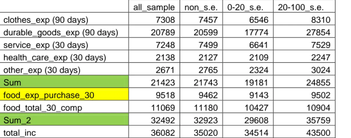
This is the mean value of expenditures by aggregated commodity groups (Table 14):

all_sample non_s.e. 0-20_s.e. 20-100_s.e. clothes_exp (90 days) 7308 7457 6546 8310 durable_goods_exp (90 days) 20789 20599 17774 27854 service_exp (30 days) 7248 7499 6641 7529 health_care_exp (30 days) 2138 2127 2109 2247 other_exp (30 days) 2671 2765 2324 3024 Sum 21423 21743 19181 24855 food_exp_purchase_30 9518 9462 9143 9502 food_total_30_comp 11069 11180 10427 10904 Sum_2 32492 32923 29608 35759 total_inc 36082 35020 34514 43500

Table 14. Final descriptive statistics of household expenditure decomposition. Sum row is the sum of previous expenditure items. Sum 2 row is Sum+ food_total_30_comp.

Food_exp_purchase_30 is part of total food expenditures. The total income below gives the idea how total expenditures and total income are related

The sample has been divided into three groups: non self - employed, people with low share of self employment income and people with high share of self - employment income (or self - employed). If we take all the people with any positive amount of self - employment income and compare them to all the sample, we can see that their expenditures do not seem to differ. On the other hand, there is high level of expenditure heterogeneity within the group of people who obtain income from self - employment. For those with high share of self - employment income (20 - 100%) the expenditures on all the types of categories are higher than both the all sample mean level (excluding food expenditures) and the people with low self - employment income share. On the other hand, the total income of self - employed is also considerably higher. So the question is whether the differences in the expenditure level may be attributed to the differences in reported income or there is some part unexplained by income variation, a part attributed to the black economy.

(27)

26

Econometric model estimation

Starting estimation the food equation let us once more provide the table of descriptive statistics for the expenditures (Table 15):

all_sample non_s.e. 0-20_s.e. 20-100_s.e. clothes_exp (90 days) 7308 7457 6546 8310 durable_goods_exp (90 days) 20789 20599 17774 27854 service_exp (30 days) 7248 7499 6641 7529 health_care_exp (30 days) 2138 2127 2109 2247 other_exp (30 days) 2671 2765 2324 3024 Sum 21423 21743 19181 24855 food_exp_purchase_30 9518 9462 9143 9502 food_exp_purchase_new_30 9976 9907 9663 10905 food_outdoors_30 1543 1718 1283 1402 food_total_30_comp 11069 11180 10427 10904 food_total_new_30_comp 11519 11625 10946 12307 sum_2 32492 32923 29608 35759 sum_3 32942 33368 30127 37162 total_inc 36082 35020 34514 43500

Table 15. Final descriptive statistics of household expenditure decomposition accounting for home made goods consumption (sum 3)

This table indicates that food expenditures based on the computation with the inclusion of home production tend to be greater for those who are self - employed, although the difference is not striking. Self - employed tend to produce and consume more goods of their own production. But the estimation of food equation in this case may turn into the estimation of the part of shadow economy attributed to the income from agricultural production, because monetary expenditures on food for self - employed and other people do not differ. Sum_3 equals the sum of all expenditures with the inclusion of home made goods consumption, sum_2 is simply the expenditure sum without the consumption of home - made goods.

As you can see from the estimation of the food equation with identifying instruments, after determining the set of appropriate instruments, the Dummy - variable indicating the self - employed type is not significant at the level of 10% (see the estimation table). The reason for this may be such that there are the household characteristics influencing food expenditures along with the level of income, but the income matters up to a certain extent, if a household is too rich it does not increase the consumption of food. However, the quadratic term of income is not significant.

It means that the food equation estimation does not give information to estimate the black economy. But we shall try to estimate the equation for the other part of expenditures. The idea is to use the part which is the most correctly reported (that is why it is not the expenditures on durable goods), and at the same time depending on income but not the structure of income. That is why we cannot use service expenditures, which include transport expenditures and are linked to the workplace. Clothes expenditures perform as the most reasonable choice as measuring the household level of welfare.

(28)

27

Here there is the estimation of food equation (Table 16). The income specification is linear, all significant variables identifying the households are kept in the model. The food expenditures are computed with the inclusion of consumption of home made goods.

The Dummy variable of self - employment is not significant on 10% significance level, therefore it does not provide any information on the estimation of the size of informal economy.

Table 16. Single food equation estimation VARIABLES ln_food_total_new_30_comp D_couple 0.124*** (0.0196) D_widow -0.0397** (0.0201) D_educ_higher -0.0525*** (0.0182) D_white_collar 0.0809*** (0.0184) D_wish_other_job 0.117*** (0.0176) D_living_improvement 0.0662** (0.0268) D_town -0.114*** (0.0184) total_square 0.000883 (0.000737) living_square 0.000974 (0.000945) D_central_water 0.0869*** (0.0275) D_phone -0.0708*** (0.0174) D_refrigerator 0.110*** (0.0172) D_washing_machine 0.0794*** (0.0214) D_plazma_TV 0.0372** (0.0183) D_DVD 0.0585*** (0.0173) D_notebook 0.0844*** (0.0192) D_computer 0.0456** (0.0185) D_bicycle 0.0797*** (0.0203) D_grown_smth 0.0655*** (0.0180) D_products_sold 0.178*** (0.0565) D_cabel_TV 0.0459** (0.0183) D_self_empl -0.0106 (0.0226) ln_Y_h 0.410*** (0.0144) Constant 4.419*** (0.136) Observations 6,192 R-squared 0.380

Standard errors inparentheses *** p<0.01, ** p<0.05, * p<0.1

(29)

28

For the clothes expenditures the dependent variable is the expenditures on clothes for both children and adults made during the last 90 days. As far as we take the log of dependent variable, its scale is not important for the estimation.

The model of clothes expenditures enables to provide the significant coefficient of the increase in the level of clothes expenditures for the self-employed compared to all the sample. To perform the clothes expenditure estimation we proceed the following way:

1) estimate the model on the full sample and call it "general";

2) identify the set of significant variables identifying the household for this sample; 3) divide the sample into the subsamples according with key types of household; 4) hold the same identifying variables in the model to obtain comparable results;

5) for each model obtain the value and significance of black economy dummy variable and the marginal propensity to consume.

Then for each subsample the black economy coefficient must be estimated. To make this we need:

1) To perform the supplementary regression for income, using exactly the same set of identifying variables. The aim is to estimate the residual error term.

2) Obtain the residual income variance estimate from STATA output as root MSE. The variance is obtained separately for the subsample of self - employed and for the subsample of employees. Along with the theory, the residual error variance for self - employed is greater than for non self-employed for all types of the models.

3) To compute the mean under - reporting parameter and the lower and upper bounds of it as determined on the base of analytical expression obtained by Pissarides and Webber.

4) With the help of these bounds we know the parameter by which the income of self employed part of households needs to be multiplied to obtain the corrected income of self - employed. 5) The mean income of self - employed and employees for each part of sample is defined and the share of self - employed households in the population.

6) The income of the self - employed is corrected with respect to this multiplier and the mean income of all sample is computed.

The bounds for the parameter of income under - estimation are computed in the tables below.