Artificial neural network modeling of water table depth fluctuations.

Artificial neural network modeling of water table depth

fluctuations

Paulin Coulibaly,

_{Franc¸ois Anctil,}

_{Ramon Aravena,}

_{and Bernard Bobe´e}

Abstract.

Three types of functionally different artificial neural network (ANN) models

are calibrated using a relatively short length of groundwater level records and related

hydrometeorological data to simulate water table fluctuations in the Gondo aquifer,

Burkina Faso. Input delay neural network (IDNN) with static memory structure and

globally recurrent neural network (RNN) with inherent dynamical memory are proposed

for monthly water table fluctuations modeling. The simulation performance of the IDNN

and the RNN models is compared with results obtained from two variants of radial basis

function (RBF) networks, namely, a generalized RBF model (GRBF) and a probabilistic

neural network (PNN). Overall, simulation results suggest that the RNN is the most

efficient of the ANN models tested for a calibration period as short as 7 years. The results

of the IDNN and the PNN are almost equivalent despite their basically different learning

procedures. The GRBF performs very poorly as compared to the other models.

Furthermore, the study shows that RNN may offer a robust framework for improving

water supply planning in semiarid areas where aquifer information is not available. This

study has significant implications for groundwater management in areas with inadequate

groundwater monitoring network.

1. Introduction

Groundwater is a significant source of drinking and domestic water in the world, especially in arid and semiarid areas. In the Sahel region (sub-Sahara west Africa), owing to the climate characterized by a short rainy season and a high evapotrans-piration, surface water is an unreliable source for water supply projects, which thereby rely mainly on groundwater. In Burkina Faso, like other Sahelian countries, the decreasing trend in rainfall since the 1970s [Ropelewski et al., 1993] and the increasing population density and related economic and domestic water demands contribute to a persistence of drought leading to larger seasonal water table fluctuations in the Sa-helian aquifers. In the framework of the United Nations Water Decade, many rural water supply projects have been carried out in the Sahel region. In Burkina Faso many wells and boreholes have been drilled in the Gondo aquifer (northwest-ern Burkina Faso). The Gondo aquifer, also referred to as the Continental Terminal aquifer, is an international groundwater system, extending from the Mouhoun River region (western Burkina Faso) to the north across the Mali border. It is the principal source of groundwater for the population in western Burkina Faso and southern Mali. A recent survey in the frame-work of the International Hydrological Program reveals that

⬃38% of the wells in the Gondo plain dry out at the end of the dry season (in March–May) [Coulibaly, 1997]. Similar observa-tions are reported in other rural areas in the Sahel region [Girard et al., 1997]. In this context, a reliable water supply planning policy, specifically during the dry season, necessitates accurately acceptable predictions of water table depth fluctu-ations. This generally requires a sufficient length of water table depth measurements, which are usually unavailable in devel-oping countries. Water table records are, in general, available only for about the last 10 years. Therefore a common approach is to use empirical time series models such as described by Box

and Jenkins [1976] and Hipel and McLeod [1994] to generate a

longer time series of water table depths. Such empirical ap-proaches have been widely used for water table depth model-ing [Tankersley et al., 1993; Van Geer and Zuur, 1997; Knotters

and van Walsum, 1997]. Unfortunately, a major disadvantage

of empirical models is that they are not adequate for making predictions when the dynamical behavior of the hydrological system changes in time [Bierkens, 1998]. This is precisely the case in the Sahelian aquifers because of the decreasing trend of rainfall and the increasing water demands. Moreover, in gen-eral, relationships between the precipitation, the nearby sur-face water, and the groundwater are likely nonlinear rather than linear. However, owing to the difficulties of identifying nonlinear model structure and estimating the associated pa-rameters, only very few nonlinear empirical models, such as stochastic differential equation and threshold autoregressive self-exciting open-loop models, have been recently proposed for shallow water table modeling [Bierkens, 1998; Knotters and

De Gooijer, 1999].

Alternatively, one can resort to descriptive (or physical) models [Belmans et al., 1983; Feddes et al., 1988]. However, in practice, the data requirements for physically based models to simulate water table fluctuation are enormous and generally difficult or costly to satisfy in many cases, particularly in de-veloping countries. Therefore a dynamical predictive model

1_{Hydro-Que´bec Chair in Statistical Hydrology, NSERC, Institut}

Na-tional de la Recherche Scientifique (INRS-Eau), Sainte-Foy, Quebec, Canada.

2_{Formerly at Department of Civil Engineering, Universite´ Laval,}

Sainte-Foy, Quebec, Canada.

3_{Department of Civil Engineering, Centre de Recherche}

Ge´oma-tique, Universite´ Laval, Sainte-Foy, Quebec, Canada.

4_{Department of Earth Sciences, University of Waterloo, Waterloo,}

Ontario, Canada.

Copyright 2001 by the American Geophysical Union. Paper number 2000WR900368.

0043-1397/01/2000WR900368$09.00

that can cope with the persistent trend and time-varying be-havior of the semiarid aquifer system is still very desirable for improved water resources management and reliable water sup-ply planning.

Recent literature reviews reveal that artificial neural net-works (ANN) specifically the feedforward netnet-works, have been successfully used for water resources variables modeling and prediction [Coulibaly et al., 1999; Maier and Dandy, 2000]. The differences of ANN-based modeling approach against the con-ventional methods are discussed in detail by many authors [Connor et al., 1994; Sarle, 1994; Weigend and Gershenfeld, 1994; Suykens et al., 1996] and specifically in hydrological ap-plications by French et al. [1992], Karunanithi et al. [1994], Hsu

et al. [1995], Tokar and Markus [2000], and Coulibaly et al.

[2000a]. Furthermore, Hornik et al. [1989] established that a three-layer feedforward ANN could be considered as a general nonlinear approximator. The major advantage of an ANN is its ability to represent underlying nonlinear dynamics of the sys-tem modeled without any a priori assumption regarding the processes involved. Recently, ANN have been successfully used for modeling complex time-varying patterns, such as low-frequency climatic oscillations [Coulibaly et al., 2000b].

In the aquifer system modeling context, ANN approach has been first used to provide maps of conductivity or transmissiv-ity values [Rizzo and Dougherty, 1994; Ranjithan et al., 1995] and to predict water retention curves of sandy soils [Schaap

and Bouten, 1996]. More recently, ANN have been applied to

perform inverse groundwater modeling for estimation of dif-ferent parameters [Morshed and Kaluarachchi, 1998; Lebron et

al., 1999].

The purpose of this paper is to identify ANN models that can capture the complex dynamics of large water table fluctu-ations, even with relatively short length of training (or calibra-tion) data. We specifically focus on temporal neural networks, such as the input delay (IDNN) and the recurrent neural net-work (RNN) that have different dynamically driven properties. In addition, emphasis is given to evaluating the ability of non-linear radial basis function (RBF) networks for water table modeling with limited data. The remainder of the paper is organized as follows. Section 2 provides a brief description of the study area and the experiment data. In section 3 we intro-duce the architecture and learning algorithm of the temporal neural networks and the RBF networks. Section 4 outlines the procedure of designing the ANN models for water table depth modeling. In section 5, results from the modeling experiment are reported and discussed. Finally, section 6 concludes the presentation.

2. Study Area and Data

The study area is located in the Gondo plain (Figure 1), northwestern Burkina Faso. The Gondo plain is part of the vast African peneplain where weathering and erosion resulted in flat plains which are sparsely to moderately vegetated. The mean elevation is⬃280 m above sea level. The climate is dry tropical with a single rainy season lasting from May to October. Mean annual precipitation is⬃700 mm but varies considerably from one year to another. The interannual rainfall variability is associated more with changes in the length of the season than changes in the intensity of the rainy season. Average air tem-perature ranges from⬃22⬚C in December–January to ⬃35⬚C in March–April. Estimated potential evapotranspiration ex-ceeds 2000 mm yr⫺1_{[Groen et al., 1988]. The Mouhoun River,}

formerly known as the Volta Noire River, is the only perennial river in the study area and in Burkina Faso. All its tributaries are temporary, flowing intermittently only from June to Sep-tember, depending on the intensity of the rains.

We selected time series of weekly water table depth records obtained from four observation wells located in the south of the Gondo plain, near the Mouhoun River and the meteoro-logical station of Solenzo (Figure 1, bottom). Daily averaged precipitation and daily minimum, maximum, and mean tem-perature series were available for the period 1970 –1997. Weekly averaged time series of the Mouhoun River water level, routinely recorded since 1980 near the study area, were available from the French Institute for Research and Devel-opment (IRD). For all the variables considered, we used monthly averaged time series, all having a length of 10 years (1986–1996), without year 1993, which had an incomplete record and was therefore dropped. The monthly averaged data are less noisy than raw daily or weekly records and seem more appropriate for long-term or seasonal forecasting [World

Me-teorological Organization (WMO), 1994]. It is noteworthy that

the two first wells selected (termed wells 1 and 2) have rela-tively large water table fluctuations, with water table depth varying from ⫺15 to ⫺2 m below ground surface. The two other wells (termed wells 3 and 4) are nearer the Mouhoun River and have smaller water table fluctuations; the ground-water level fluctuates from⫺9 to ⫺3 m below the soil surface. Figure 2 shows the averaged monthly water table depth fluc-tuations for wells 1 and 3 with regard to the monthly precipi-tation of the same period (1986–1996). Figure 2 suggests that precipitation and thereby intermittent surface water are the dominant recharge processes in the study area. However, it is thought that some proportion of the groundwater derives from the Mouhoun River specifically during the dry season

[Couli-baly, 1997].

The Gondo plain is entirely underlain by the Continental Terminal, a nonmarine sedimentary deposit of 20–100 m thick-ness, considered to be Tertiary in age. It consists mostly of argillaceous and sandy sediments with some clay, silt, and gravel. Therefore the selected water table depth series are geohydrologically representative of many possible situations throughout the Gondo plain. Indeed, most of the villages are traditionally established where the groundwater level was mod-erately deep and thus reachable even by dug wells.

3. ANN Models

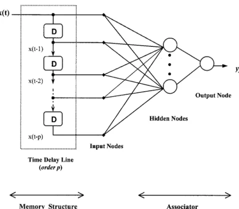
3.1. Input Delay Neural Network

The basic IDNN consists of two components: a memory structure and a nonlinear associator. Figure 3 depicts the ar-chitecture of the IDNN used in this study. The memory struc-ture is a time delay line which corresponds to a buffer contain-ing the p most recent inputs generated by the delay unit operator D, while the associator is the conventional feedfor-ward network with one hidden layer and one output layer. The memory structure holds on to the relevant past information, and the associator uses the memory to predict future events. A particular feature of the IDNN is that the memory structure is focused on the input layer; this makes it different from the general time delay neural network (TDNN) [Waibel et al., 1989; Wan, 1994], which uses internal delays at each neuron. A major advantage of the IDNN is that it is less complex than the conventional TDNN and has the same temporal patterns pro-cessing capability [Clouse et al., 1997]. Furthermore, the IDNN

can be trained even by using the standard backpropagation algorithm [Rumelhart et al., 1986]. Here the output of the IDNN assuming a linear output neuron j, a single hidden layer with h sigmoid hidden nodes (or computational units), and an input variable x(t) is given by

yj⫽ F

冉

冘

i⫽1 h

wjiG共si兲 ⫹ bj

冊

where F( ) is the linear activation function of the output neuron j and bj is its bias (or threshold), wji represents the

synaptic weight connecting the hidden unit i to the output unit

j, G( ) is the logistic function, which is the most often used

form of the sigmoid activation function for the hidden nodes, and can be expressed

G共si兲 ⫽ 关1 ⫹ exp 共⫺si兲兴⫺1, (2)

where siis the weighted sum of all incoming information for

neuron i and is also referred to as the input signal:

si共t兲 ⫽

冘

k⫽0 p

wi共k兲 x共t ⫺ k兲 ⫹ bi⫽ wix, (3)

where p is the time delay line memory length, also termed memory order p, wiis the weight vector for the ith hidden unit

and biis its threshold (or bias) which is an offset for the input

signal, and x denotes the vector of delayed inputs from the time delay line. For optimization purposes, we use a second-order backpropagation variation, namely, the Levenberg-Marquardt backpropagation for the IDNN training. In

tice, this training method has been found effective in finding better optima than the standard backpropagation and the con-jugate gradient descent method [Hagan and Menhaj, 1994;

Coulibaly et al., 2000a].

3.2. Recurrent Neural Network

The RNN used in this study is the basic Elman type RNN [Elman, 1990] also referred to as the globally connected RNN. The network consists of four layers (Figure 4): an input layer with five nodes, a hidden layer with three nodes, a context layer with three units, and an output layer with one node. Each input unit is connected to every hidden unit, as is each context unit. Conversely, there are one-by-one downward connections be-tween the hidden nodes and the context units leading to an equal number of hidden and context units. In fact, the down-ward connections allow the context units to store the outputs of the hidden nodes (i.e., internal states) at each time step; then the fully distributed upward links feed them back as additional inputs. Therefore the recurrent connections allow the hidden units to recycle the information over multiple time steps and thereby to discover temporal information contained in the sequential input and relevant to the target function. Thus the RNN has an inherent dynamic (or adaptive) memory provided by the context units in its recurrent connections. Finally, here the output of the network depends not only on the connection weights and the current input signal but also on the previous states of the network, as follows:

yj⫽ Axⴕ共t兲 (4)

xⴕ共t兲 ⫽ G关Whxⴕ共t ⫺ 1兲 ⫹ Wh0x共t ⫺ 1兲兴 (5)

where xⴕ(t) is the output of the hidden layer at time t given an input vector x(t), G( ) denotes a logistic function

character-izing the hidden nodes, the matrix Whrepresents the weights of

the h hidden nodes that are connected to the context units, Wh0

is the weight matrix of the hidden units connected to the input nodes, yjis the output of the RNN assuming a linear output

node j, and A represents the weight matrix of the output layer neurons connected to the hidden neurons. The Elman-style RNN is a state-space model since (5) performs the state esti-mation and (4) performs the evaluation.

A major difficulty when using RNN is the training complex-ity because the computation of ⵜE(w), the gradient of the error E with respect to the weights, is not trivial since the error is not defined at a fixed point but rather is a function of the network temporal behavior. Here we specifically make use of a variant of temporal back propagation, namely, the back prop-agation through time (BPTT) variation proposed by Williams

and Peng [1990]. This algorithm uses a continuous mode of

training in which the adjustment of the weights is made at each time step and only the relevant history of the input patterns and the network states for a fixed number of time steps, called the truncation depth, are saved. Thereby the algorithm is also referred to as the truncated BPTT. In practice, this method is considered as the best on-line technique for practical problems [Pearlmutter, 1995] and has been widely used to train RNN to perform various tasks [Williams and Zipser, 1995; Puskorius et

al., 1996; Feldkamp and Puskorius, 1998; Coulibaly et al., 2001].

A comprehensive description of the truncated BPTT is pro-vided by Haykin [1999].

3.3. Radial Basis Function Networks

Two variants of RBF are considered in this study, a gener-alized radial basis function network (GRBF) and a variation of RBF network named probabilistic neural network (PNN). The former represents the general and typical form of RBF

work, while the latter is a variation of RBF network that uses a soft competitive activation function derived from the Bayes-ian classification theory. Even though both networks assume Gaussian (or radial) basis functions for their hidden units, they have different advantages that lead to their choice. The PNN has the advantage of being robust in the presence of noise [Wasserman, 1993, p. 53], whereas the GRBF combines the advantage of generality and reduced computational complexity [Specht, 1991], but it is not good at ignoring irrelevant inputs.

Furthermore, it has been shown that RBF networks with a single hidden layer of Gaussian units are universal approxima-tors [Park and Sandberg, 1991].

Basically, a RBF network has three layers (Figure 5). The input layer that simply passes the inputs to a single hidden layer which performs a nonlinear transformation from the in-put space to the hidden (or feature) space. The response of the network is supplied by a linear output layer for the GRBF and by a competitive output layer for the PNN. The typical RBF

Figure 3. Input delay neural network architecture with p memory order.

network (Figure 5) looks like the conventional three-layer feedforward network topology; however, its operation is fun-damentally different. The learning scheme of feedforward back propagation network can be viewed as a stochastic approxima-tion, whereas the learning of RBF network is equivalent to finding an optimum surface in a multidimensional space. Con-sidering the GRBF (Figure 5), given an input variable xk, each

hidden unit output␸iis obtained by computing the Euclidean

distance between the input vector and the connection weight vector wifor the ith hidden unit, as follows:

␸i共 xk兲 ⫽ ⌽

冉

␴i

冊

where⌽ is a strictly positive radially symmetric function known as radial basis function, which is assumed here to be a Gaussian exponential, ␴i represents the smoothing parameter of the

Gaussian basis function for the neuron i, and储 储 denotes the Euclidean norm. Note that there are as many hidden units (or radial basis neurons) as there are input vectors in the training data. Here the final output of the GRBF is given by the linear output neuron as

yj⫽

冘

i⫽1 h

wji␸i共 xq兲 ⫽ WjT␸, (7)

where yjis a linearly weighted sum of the outputs of the hidden

units, WjTis the weight vector for the output neuron j,␸ is the

vector of outputs from the hidden layer, and T indicates the transpose operation. For the RBF network to perform a spe-cific nonlinear input-output mapping, it must be trained on a set of known input-output examples. Here the supervised gra-dient descent–based method [Poggio and Girosi, 1990] is used for the network training. In this training procedure the error function E is minimized by adaptively updating all the free parameters (wi, ␴i, and wji) of the network. In fact, the

training consists of adapting the centers of the radial basis neurons (i.e., hidden units). A GRBF network trained by the supervised gradient descent algorithm has been found capable of exceeding substantially the generalization performance of

standard back propagation–trained networks [Wettschereck

and Dietterich, 1992].

The probabilistic neural network (PNN) [Specht, 1990;

Was-serman, 1993] is an RBF network that approximates the

Bayes-ian decision rule. The PNN architecture is similar to that of the GRBF except that the linear output layer is replaced by a competitive layer. Like the GRBF, the PNN shares the con-straint of having an equal number of hidden units and input patterns. Given a training example {xk, dk} of input vector xk

and desired (or target) vector dk, the hidden units’ weights wi

are updated according to the recursion

⌬wi⫽␳共xk⫺ wi兲␸i共xk兲, (8)

where 0⬍␳ ⬍ 1 and ␸i( xk) is the output of the ith hidden

unit. Here all the hidden nodes or basis functions are assumed to be Gaussian exponentials with identical width (or smooth-ing) parameter␴. Therefore, while the parameter ␴ tends to zero, only the hidden unit whose weight best matches the input vector xk is updated. Conversely, for the nonzero ␴, all the

hidden units’ weights are updated. In fact, this procedure can be considered as an iterative realization of the maximum like-lihood estimate for wi. Next, the competitive output layer sums

the outputs of the hidden nodes for each class of inputs to form a vector of probabilities. Then the maximum of these proba-bilities is picked as the final output.

Basically, PNN memorizes all the training patterns. While a new input pattern is presented to the network, it computes the output for all the hidden nodes, sums up the resulting outputs classwise, and finally selects the output that had the maximum probability of being correct. PNN generalization performance depends heavily on the value of the smoothing parameter ␴ and on how well the training data represents the system being modeled. PNN has been recently found more suitable for stock trend prediction, which does not require training on long his-tory data [Saad et al., 1998].

4. Network Design for the Modeling Experiment

ANN topology is problem dependent. Whatever the type of ANN model used, it is important to determine the appropriate

network architecture in order to obtain satisfactory generali-zation capability. Here the networks are developed using the Neural Network Toolbox 3 (The Mathworks Inc., Natick, Mas-sachusetts). For the IDNN we first used the water table depth

XWTDrecords and all the five hydrometeorological input vari-ables, namely, the precipitation Xp; the Mouhoun River water

level XMWL; the maximum, minimum and mean temperature

(XTmx, XTmn, XTm, and respectively), to identify the optimum

IDNN architecture using the common trial-and-error method. Different lengths of the input delay memory varying from 1 to 4 months has been tested with varied number of hidden nodes. It is found that five hidden nodes are the optimum with an input delay memory p⫽ 2 in this experiment. Note that a time

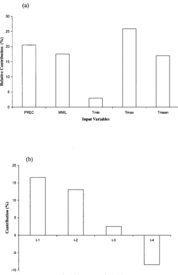
delay line with an order p ⫽ 2 is, in fact, a short-term static memory structure since a particular feature of the IDNN is that the selected delay order is not adjustable during the net-work learning. Figure 6b shows the relative contribution for the different delay order tested. In this case, a contribution ⬍5% is not significant in terms of model performance. It can be seen from Figure 6b that a delay memory p ⱖ 3 does not provide significant contribution to the model performance; it appears to be rather counterproductive for the model. Next, using the IDNN with five sigmoid hidden nodes and p ⫽ 2, a sensitivity analysis is carried out to assess the relative signifi-cance of each hydrometeorological input variable. Figure 6a shows the relative contribution of each input variable to the model performance. Maximum temperature and precipitation seem to be the dominant patterns, while the Mouhoun River water level and the mean temperature have slightly equivalent significance. Minimum temperature is the least significant vari-able in the data set and is therefore deleted. Note that using the IDNN, the same delay memory order (here p ⫽ 2) is applied to all the selected five input variables. Architectural description of the models selected for the water table modeling experiment is presented in Table 1. Each model structure is represented by the notation n-h-o, where n is the number of input nodes, h is the number of hidden nodes, and o is the number of output nodes. For example, the IDNN model has 15 (n⫽ 15) input variables, five sigmoid hidden nodes (h ⫽ 5), and one linear output node (o ⫽ 1).

For the RNN, only the selected five input variables are provided to the network as shown in Figure 4. The inherent internal recurrence allows the network to incorporate past information relevant to the target function. An important fea-ture of RNN is its adaptive memory provided by the context units discussed previously. Therefore, in general, there is no need for an external memory structure, such as input time delay or sliding window.

Determining an appropriate architecture for a RBF network reduces to selecting relevant input patterns. Careful inputs selection for the RBF network is essential because of the constraint of having as many hidden nodes as input vectors. Therefore it is straightforward that such a model can suffer from the curse of dimensionality. Furthermore, irrelevant in-put acts as noise in the data, leading to a poor network gen-eralization, specifically for the GRBF. Therefore, for both the GRBF and the PNN, different moving windows of inputs based on the five input variables previously selected have been con-sidered. In this experiment, it is found that in addition to the five input variables, only the previous month maximum tem-perature and water table depth seem to be relevant to the RBF networks performance. Therefore a moving window of seven input variables is used as shown in Figure 5, and thereby seven

Figure 6. Relative contribution of input variables and differ-ent delay memory order.

Table 1. Architectural Description of the Selected ANN Modelsa

Model Memory Order p Memory Structure Architecture(n-h-o) ParametersNumber of

IDNN p ⫽ 2 (static) time delay 15-5-1 86

RNN pⱖ 1 (adaptive) recurrent connections (context units) 5-3-1 31

GRBF p ⫽ 1 (static) moving window 7-7-1 56

PNN p ⫽ 1 (static) moving window 7-7-1 56

a_{ANN, artificial neural network; IDNN, input delay neural network; RNN, recurrent neural network;}

GRBF, generalized radial basis function; PNN, probabilistic neural network; n, number of input nodes;

hidden units are used in the hidden layer. RBF networks are nonlinear static networks; to enable such models for future water table prediction, a memory structure is needed. Thus the networks are trained using the moving window of selected inputs. This provides the network with a short-term static memory. For the GRBF the smoothing parameter is initially set to␴ ⫽ 0.25 and is progressively updated during the super-vised training procedure, whereas for PNN, different smooth-ing parameters rangsmooth-ing from␴ ⫽ 0.05 to ␴ ⫽ 0.5 with a step of 0.05 are tested, and finally,␴ ⫽ 0.1 is selected. Each of the selected RBF networks has a total of 56 parameters (weights), while the IDNN and the RNN have 86 and 31 parameters, respectively (Table 1).

For all the selected ANN models we used 7 years (1986– 1992) of monthly data for the model training (calibration) and 3 years (1994–1996) for the validation. The network training is stopped when the training error has reached a sufficiently small value (termed “error goal”) and changes in the predic-tion error remain very small. The common iterative multistep ahead forecasting method as described by Coulibaly et al. [2000a] is used to predict the water table up to 3 months ahead. Such predictions are particularly needed for reliable water supply planning during the dry season. Some results of the prediction experiment are discussed in section 5.

To evaluate the model performance, the root mean square error (RMSE) is selected as it shows the global goodness of the fit. Here, as the forecast accuracy for deep water table is of particular interest for water supply planning during the dry season, a large water table depth criterion termed LDC is introduced and can be computed by

LDC⫽

冉

冘

冊

冉

冘

冊

where TLis the number of large water table depths larger than

one half of the mean large water table depth observed and yt

and yˆt are the observed and computed water table depths,

respectively. LDC provides accurate measure of the model performance for the dry period. Note that a LDC equal to zero represents a perfect fit, whereas a LDC value⬎0.2 implies a prediction error greater than⫾1 m for deep water table. This indicates a rather poor model performance for dry season water table forecasting in this case.

5. Results and Discussion

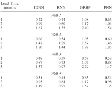
The RMSE and LDC statistics of the identified models for the 3 year test period (1994–1996) are summarized in Tables 2 and 3, respectively. In general, it can be seen from Table 2 that all the models perform relatively better for the moderate (or small) water table fluctuations (wells 3 and 4) than the large water table fluctuations (wells 1 and 2). This may indicate that larger fluctuations of groundwater level are likely more diffi-cult to predict. However, the prediction results obtained for the large water table fluctuations are relatively good depending on the model. It is clear from Table 2 that whatever the fore-cast lead time, the RNN outperforms all the other ANN mod-els. In general, the IDNN and the PNN have, on average, equivalent prediction performance despite their basically

dif-ferent learning scheme. However, the PNN slightly outper-forms the IDNN for the large water table fluctuations model-ing. Conversely, the IDNN seems, in general, fairly better than the PNN for the moderate water table fluctuations prediction. The GRBF performs poorly with comparison to the other models. This may suggest that the general form of RBF net-work may not be suitable for water table modeling based on short length calibration data. However, one can argue that the presence of noise is unavoidable in real-world data, such as rainfall, river water level, and temperature series. Since the GRBF is very sensitive to the presence of noise in the training data, this may explain its poor performance in this experiment. Conversely, the PNN, which is more robust in the presence of noisy training data, clearly exhibits better potential for the water table modeling. Further analysis of Table 2 reveals that the prediction error in terms of RMSE increases rapidly with the growth of the forecast lead time for all the models. For 1

Table 2. Comparative Performance of ANN Models in Terms of RMSEa Lead Time, months IDNN RNN GRBF PNN Well 1 1 0.72 0.44 1.08 0.63 2 0.99 0.60 1.17 1.04 3 1.67 1.35 2.40 1.54 Well 2 1 0.68 0.54 1.05 0.60 2 1.47 1.29 1.57 1.46 3 1.70 1.44 1.97 1.85 Well 3 1 0.48 0.39 0.67 0.58 2 0.87 0.73 1.07 0.88 3 1.37 0.97 2.29 1.47 Well 4 1 0.51 0.44 0.63 0.54 2 0.95 0.84 1.17 0.98 3 1.19 0.95 1.57 1.35

a_{Performance values are in meters.}

Table 3. Comparative Performance of ANN Models in Terms of LDC Lead Time, months IDNN RNN GRBF PNN Well 1 1 0.11 0.10 0.16 0.14 2 0.19 0.11 0.18 0.20 3 0.22 0.16 0.30 0.26 Well 2 1 0.12 0.09 0.17 0.10 2 0.20 0.16 0.20 0.20 3 0.20 0.17 0.27 0.26 Well 3 1 0.12 0.10 0.14 0.11 2 0.15 0.13 0.16 0.15 3 0.18 0.15 0.25 0.20 Well 4 1 0.12 0.11 0.14 0.11 2 0.15 0.14 0.17 0.16 3 0.17 0.15 0.19 0.19

month ahead forecast, all the models have good predictions except the GRBF model, which has satisfactory predictions only for wells 3 and 4, while for 2 month ahead forecast, the IDNN and the RNN substantially outperform the RBF net-works. Only the RNN shows a potential for the 3 month ahead forecast experiment, suggesting that this model can be used to anticipate whether a shortage of water can occur in the next 3 months.

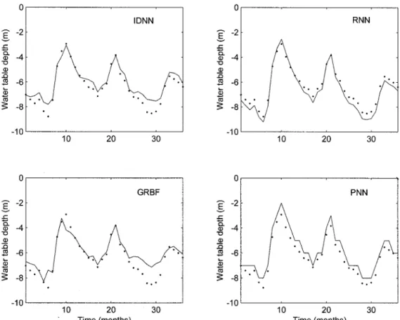
To assess the model prediction performance specifically dur-ing the dry season, the LDC statistics are shown in Table 3. The LDC statistics reveal that for 1 month ahead forecast, all the proposed models can provide satisfactory predictions (LDC⬍ 0.2) for both large and moderate water table fluctu-ations. More interestingly, both the temporal networks (RNN and IDNN) and the PNN are effective for deep water table predictions up to 2 and 3 month ahead for wells 3 and 4. However, for wells 1 and 2, only the RNN performs very well for 2 and 3 month ahead forecast during the dry period. The IDNN and the PNN have similar performance for 2 month ahead forecast of deep water table, but the IDNN substantially outperforms the PNN for the 3 month ahead forecast of large water table depths. Recall that the RNN is the most parsimo-nious model with 31 parameters; therefore its good results indicate that dynamical modeling capabilities of globally RNN are substantially better than those of static memory models, such as IDNN and RBF networks even with moving window. In general, whatever the ANN models used, the prediction results for wells 1 and 2 are relatively similar as are those for wells 3 and 4 (Tables 2 and 3). Therefore further results dis-cussion will be illustrated either by wells 1 and 3 or wells 2 and 4. Figures 7 and 8 show the results of 1 month ahead prediction

for wells 1 and 3, respectively. Figure 7 confirms that the RNN and the IDNN are more effective at forecasting both the mag-nitude and the timing of deep water table (less than⫺6 m in average) than shallow water table. As accurate prediction of the dry season deep water table is particularly important for reliable water supply planning; thus the results from Figure 7 are very encouraging. For the moderate water table fluctua-tions (Figure 8), all the models tend to underpredict the deep water table except RNN, which slightly overpredict the deep water table. Note that here overprediction denotes more neg-ative depth than measured, whereas underprediction means an observation depth more negative than predicted. In this case, overprediction is preferable to underprediction because it of-fers better reliability. Therefore the RNN seems to be the more suitable for modeling both the large and small water table fluctuations. These results also suggest that RNN do not necessarily require a longer sample as is required by linear models in order to perform well.

To further substantiate the potential of RNN for long-term forecast, Figure 9 presents the 3 month ahead prediction de-viations from the observed water table depths (wells 2 and 4) using the RNN model. Positive deviation values indicate that the model overpredicts the water level, whereas negative de-viation values denote underprediction. In general, Figure 9 shows that the RNN model tends to overpredict the water table depth. This can be generally acceptable specifically for the deep depth prediction as discussed previously. Owing to the large fluctuation of water level in the study area a 3 month prediction error less than⫾1 m is very satisfactory. It can be seen from Figure 9 that on average, 60% of the 3 month ahead forecasts are acceptable. For the moderate water table

fluctu-Figure 7. Results of 1 month ahead prediction (solid line) and observed water table depths (points) for well 1.

ations (well 4),⬃75% of the 3 month ahead predictions are satisfactory, whereas for the larger water table fluctuations (well 2), 55% of the predictions are good. These results suggest that the RNN model can offer a reliable framework for water table fluctuations modeling.

6. Conclusions

This study has shown that temporal and probabilistic neural networks are effective at predicting monthly groundwater level

fluctuations in the Gondo aquifer located in the Sahel region. A significant advantage of these models is that they can pro-vide satisfactory predictions with short groundwater level records, which are a common occurrence in countries with scarce instrumentation for groundwater monitoring. It is found that the Elman-type RNN trained with a truncated BPTT is the most suitable for both deep and shallow water table modeling. The prediction results suggest that the RNN can be an effec-tive tool for up to a 3 month ahead forecast of the dry season deep water table depths. Conversely, the prediction results indicate that the general form of RBF network (GRBF) is not appropriate to deep water table modeling, whereas the IDNN and the PNN are relatively effective for up to 2 month ahead predictions.

The optimum ANN-based model proposed in this study shows very promising results for improving water supply plan-ning in semiarid areas. The experimental results suggest that the RNN model can offer a reliable framework for water table fluctuations modeling where (1) there is no need for internal aquifer system modeling, (2) aquifer system information is not available to run a descriptive model, and (3) the available data records are relatively short. Furthermore, the model perfor-mance can likely be improved by considering additional infor-mation, such as demographic factors, water withdrawal, and evapotranspiration rates. More interestingly, the model is less costly and can be applied to any rural water supply planning where limited water table depth measurements are available.

Acknowledgments. This study was made possible through a grant from the Rockefeller Foundation to P.C. This support is gratefully acknowledged. Part of this research was funded by a grant from the

Figure 8. Results of 1 month ahead prediction (solid line) and observed water table depths (points) for well 3.

Figure 9. Three month ahead prediction deviations from ob-served water table depths using RNN model.

Natural Sciences and Engineering Research Council of Canada to F.A. The authors would like to thank the National Meteorology Institute of Burkina Faso and the French Institute for Research and Development (IRD) for providing the experiment data. We thank the three review-ers, Marcel Schaap, Martin Knottreview-ers, and S. Ranji Ranjithan, for their comments, which helped to improve the original document.

References

Belmans, C., J. G. Wesseling, and R. A. Feddes, Simulation of water balance of a cropped soil: SWATRE, J. Hydrol., 63, 271–286, 1983. Bierkens, M. F. P., Modeling water table fluctuations by means of a stochastic differential equation, Water Resour. Res., 34(10), 2485– 2499, 1998.

Box, G. E. P., and G. M. Jenkins, Time Series Analysis: Forecasting and

Control, Holden-Day, Boca Raton, Fla., 1976.

Clouse, D. S., C. L. Giles, B. G. Horne, and G. W. Cottrell, Time-delay neural networks: Representation and induction of finite-state ma-chines, IEEE Trans. Neural Networks, 8(5), 1065–1070, 1997. Connor, J. T., R. D. Martin, and L. E. Atlas, Recurrent neural

net-works and robust time series prediction, IEEE Trans. Neural

Net-works, 5(2), 240–254, 1994.

Coulibaly, P., Gondo plain: Water quality and water resources man-agement methods in the villages (in French), Res. Rep. SC/RP

205.028.6, 40 pp., UNESCO, Paris, France, 1997.

Coulibaly, P., F. Anctil, and B. Bobe´e, Hydrological forecasting using artificial neural networks: The state of the art (in French), Can. J.

Civ. Eng., 26(3), 293–304, 1999.

Coulibaly, P., F. Anctil, and B. Bobe´e, Daily reservoir inflow forecast-ing usforecast-ing artificial neural networks with stopped trainforecast-ing approach,

J. Hydrol., 230, 244–257, 2000a.

Coulibaly, P., F. Anctil, P. F. Rasmussen, and B. Bobe´e, A recurrent neural networks approach using indices of low-frequency climatic variability to forecast regional annual runoff, Hydrol. Processes,

14(15), 2755–2777, 2000b.

Coulibaly, P., F. Anctil, and B. Bobe´e, Multivariate reservoir inflow forecasting using temporal neural networks, J. Hydrol. Eng., in press, 2001.

Elman, J. L., Finding structure in time, Cognitive Sci., 14, 179–211, 1990.

Feddes, R. A., P. Kabat, P. J. T. Van Bakel, J. J. B. Bronswijk, and J. Halbertsma, Modeling soil water dynamics in the unsaturated zone—State of the art, J. Hydrol., 100, 69–111, 1988.

Feldkamp, L. A., and G. V. Puskorius, A signal processing framework based on dynamic neural networks with application to problems in adaptation, filtering and classification, Proc. IEEE, 86(11), 2259– 2277, 1998.

French, M. N., W. F. Krajewski, and R. R. Cuykendall, Rainfall fore-casting in space and time using a neural network, J. Hydrol., 137, 1–31, 1992.

Girard, P., C. HillaiMarcel, and M. S. Oga, Determining the re-charge mode of Sahelian aquifers using water isotopes, J. Hydrol.,

197, 189–202, 1997.

Groen, J., J. B. Schuchmann, and W. Geirnaert, The occurrence of high nitrate concentration in groundwater in villages in northwest-ern Burkina Faso, J. Afr. Earth Sci., 7(7–8), 999–1009, 1988. Hagan, M. T., and M. B. Menhaj, Training feedforward networks with

the Marquardt algorithm, IEEE Trans. Neural Networks, 5(6), 989– 993, 1994.

Haykin, S., Neural Networks: A Comprehensive Foundation, Prentice-Hall, Old Tappan, N. J., 1999.

Hipel, K. W., and A. I. McLeod, Time Series Modelling of Water

Re-sources and Environmental Systems, Dev. Water Sci., vol. 45, Elsevier

Sci., New York, 1994.

Hornik, K., M. Stinchcombe, and H. White, Multilayer feedforward networks are universal approximators, Neural Networks, 2(5), 359– 366, 1989.

Hsu, K. L., H. V. Gupta, and S. Sorooshian, Artificial neural network modeling of the rainfall-rainoff process, Water Resour. Res., 31(10), 2517–2530, 1995.

Knotters, M., and J. G. De Gooijer, TARSO modeling of water table depths, Water Resour. Res., 35(3), 695–705, 1999.

Knotters, M., and P. E. V. van Walsum, Estimating fluctuation quan-tities from time series of water-table depths using models with a stochastic component, J. Hydrol., 197, 25–46, 1997.

Lebron, L., M. G. Schaap, and D. L. Suarez, Saturated hydraulic

conductivity prediction from microscopic pore geometry measure-ments and neural networks analysis, Water Resour. Res., 35(10), 3149–3158, 1999.

Maier, H. R., and G. C. Dandy, Neural networks for the prediction and forecasting of water resources variables: A review of modelling is-sues and applications, Environ. Model. Software, 15, 101–124, 2000. Morshed, J., and J. J. Kaluarachchi, Parameter estimation using arti-ficial neural network and genetic algorithm for free-product migra-tion and recovery, Water Resour. Res., 34(5), 1101–1113, 1998. Park, J., and I. W. Sandberg, Universal approximation using

radial-basis-function networks, Neural Comput., 3, 246–257, 1991. Pearlmutter, B. A., Gradient calculations for dynamic recurrent neural

networks: A survey, IEEE Trans. Neural Networks, 6(5), 1212–1228, 1995.

Poggio, T., and F. Girosi, Networks for approximation and learning,

Proc. IEEE, 78, 1481–1497, 1990.

Puskorius, G. V., L. A. Feldkamp, and L. I. Davis, Dynamic neural network methods applied to on-line vehicle idle speed control, Proc.

IEEE, 34, 1407–1420, 1996.

Ranjithan, R. S., J. W. Eheart, and J. H. Garrett, Application of neural network in groundwater remediation under conditions of uncer-tainty, in New Uncertainty Concepts in Hydrology and Water

Re-sources, edited by Z. W. Kundzewicz, pp. 133–140, Cambridge Univ.

Press, New York, 1995.

Rizzo, D. M., and D. E. Dougherty, Characterization of aquifer prop-erties using artificial neural networks: Neural kriging, Water Resour.

Res., 30(2), 483–497, 1994.

Ropelewski, C. F., P. J. Lamb, and D. H. Portis, The global climate from June to August 1990: Drought returns to sub-Saharan West Africa and warm Southern Oscillation episode conditions develop in the central Pacific, J. Clim., 6, 2188–2212, 1993.

Rumelhart, D. E., G. E. Hinton, and R. J. Williams, Learning internal representation by error propagation, in Parallel Distributed

Process-ing: Explorations in the Microstructure of Cognition, vol. 1, edited by

D. E. Rumelhart and J. L. McClelland, pp. 318–362, MIT Press, Cambridge, Mass., 1986.

Saad, E. W., D. V. Prokhorov, and D. C. Wunsch, Comparative study of stock trend prediction using time delay, recurrent and probabi-listic neural networks, IEEE Trans. Neural Networks, 9(6), 1456– 1470, 1998.

Sarle, W. S., Neural networks and statistical models, in Proceedings of

the Nineteenth Annual SAS Users Group International Conference, pp.

1538–1550, SAS Inst., Cary, N. C., 1994.

Schaap, M. G., and W. Bouten, Modeling water retention curves of sandy soils using neural networks, Water Resour. Res., 32(10), 3033– 3040, 1996.

Specht, D. F., Probabilistic neural networks, Neural Networks, 3(1), 109–118, 1990.

Specht, D. F., A general regression neural network, IEEE Trans.

Neu-ral Networks, 2(6), 569–576, 1991.

Suykens, J. A. K., J. P. L. Vandewalle, and B. L. R. De Moor, Artificial

Neural Networks for Modelling and Control of Nonlinear Systems,

Kluwer Acad., Norwell, Mass., 1996.

Tankersley, C. D., W. D. Graham, and K. Hatfield, Comparison of univariate and transfer function models of groundwater fluctuations,

Water Resour. Res., 29(10), 2517–3533, 1993.

Tokar, A. S., and M. Marcus, Precipitation-runoff modeling using artificial neural networks and conceptual models, J. Hydrol. Eng.,

5(2), 156–161, 2000.

Van Geer, F. C., and A. F. Zuur, An extension of Box-Jenkins transfer/ noise models for spatial interpolation of groundwater head series, J.

Hydrol., 192, 65–80, 1997.

Waibel, A., T. Hanazawa, G. Hintin, K. Shikano, and K. J. Lang, Phoneme recognition using time delay neural networks, IEEE Trans.

Acoust. Speech Signal Process., 37(3), 328–339, 1989.

Wan, E., Time series prediction using a connectionist network with internal delay lines, in Time Series Prediction: Forecasting the Future

and Understanding the Past, edited by A. S. Weigend and N. A.

Gershenfeld, pp. 195–217, Addison-Wesley-Longman, Reading, Mass., 1994.

Wasserman, P. D., Advanced Methods in Neural Computing, Van Nos-trand Reinhold, New York, 1993.

Weigend, A. S., and N. A. Gershenfeld (Ed.), Time Series Prediction:

Forecasting the Future and Understanding the Past,

Addison-Wesley-Longman, Reading, Mass., 1994.

radial basis function networks by learning center locations, Adv.

Neural Inf. Processing Syst., 4, 1133–1140, 1992.

Williams, R. J., and J. Peng, An efficient gradient-based algorithm for on-line training of recurrent network trajectories, Neural Comput., 2, 490–501, 1990.

Williams, R. J., and D. Zipser, Gradient-based learning algorithms for recurrent neural networks and their computational complexity, in

Back Propagation: Theory, Architectures, and Applications, edited by

Y. Chauvin and D. E. Rumelhart, pp. 433–486, Lawrence Erlbaum Assoc., Hillsdale, N. J., 1995.

World Meteorological Organization (WMO), Guide for hydrological practices, Geneva, Switzerland, 1994.

F. Anctil, Department of Civil Engineering, Centre de Recherche Ge´omatique, Universite´ Laval, Sainte-Foy, Quebec, Canada G1K 7P4. R. Aravena, Department of Earth Sciences, University of Waterloo, Waterloo, Ontario, Canada N2L 3G1.

B. Bobe´e and P. Coulibaly, NSERC/Hydro-Que´bec Chair in Statis-tical Hydrology, Institut National de la Recherche Scientifique (INRS-Eau), Sainte-Foy, Quebec, Canada G1V 4C7. (Paulin_Coulibaly@ inrs-eau.uquebec.ca)

(Received March 31, 2000; revised November 7, 2000; accepted November 9, 2000.)