This is an author-deposited version published in: http://oatao.univ-toulouse.fr/
Eprints ID: 5787
To link to this article: DOI: 10.1016/j.jfi.2008.09.002
URL: http://dx.doi.org/10.1016/j.jfi.2008.09.002
To cite this version:
Dridi, Ramdan and Germain, Laurent Noise and
competition in strategic oligopoly. (2009) Journal of financial
intermediation, 18 (2). pp. 311-327. ISSN 1042-9573
O
pen
A
rchive
T
oulouse
A
rchive
O
uverte (
OATAO
)
OATAO is an open access repository that collects the work of Toulouse researchers and makes it freely available over the web where possible.
Any correspondence concerning this service should be sent to the repository administrator: staff-oatao@inp-toulouse.fr
Noise and Competition in Strategic Oligopoly
∗Ramdan Dridi† and Laurent Germain‡ June 2008
∗We are particularly indebted to Herv´e Boco, Bruno Biais, Gilles Chemla, Gabrielle Demange, Marcus
Brun-nermeier, Antoine Faure-Grimaud, Mike Fishman, Jean-Claude Gabillon, Andr´e Grimaud, Thomas Mariotti, Jean-Charles Rochet, and especially to David Stolin as well as seminar participants at Toulouse, the London School of Economics, the American Finance Association Meeting (2001) in New Orleans, the Western Finance Association (2001) in Tucson for long conversations and very thoughtful comments which have greatly improved the quality of this paper. All remaining errors are our own.
†Toulouse Business School, Groupe de Finance, 20 boulevard Lascrosses, BP 7010, 31068 Toulouse cedex 7,
France. Tel 33 5 61 29 49 43, Fax: 33 5 61 23 32 79, E-mail: r.dridi@esc-toulouse.fr
‡Corresponding author. Toulouse Business School, Groupe de Finance, SUPAERO and Europlace Institute of
Finance, Toulouse Business School 20 boulevard Lascrosses, BP 7010, 31068 Toulouse cedex 7, France. Tel 33 5 61 29 49 43, Fax: 33 5 61 23 32 79, E-mail: l.germain@esc-toulouse.fr
Abstract
In this paper, we propose a model where N strategic informed traders who are endowed with heterogeneous noisy signals with different precisions compete in a market with a single risky asset. We explicitly describe the unique linear equilibrium that exists in this setup and derive its properties. Moreover, we focus on the effects of noise on the competition between traders. We show that noise softens the competition between traders. In particular, for N exceeding three and for certain sets of noise in traders’ signals, each trader’s individual profit is greater than the one obtained in the case of perfect information.
Keywords: Competition, Optimal Noise, Price Manipulation. JEL Classification: D43, D82, G14, G24.
1
Introduction
Collecting and exploiting information in financial markets is one of the main activities of insti-tutions such as banks, securities houses, or hedge funds. Such instiinsti-tutions have different reasons for trading and therefore they collect information in different ways. Thus, a realistic theoretical framework for understanding competition between different informed traders would endow these agents with different signals stemming from different distributions. However, most models in the literature consider that traders’ information is homogeneous and collected signals are the same or that signals are heterogeneous but following the same distributions. In our paper, the collected signals are heterogeneous and stem from different distributions. Thus it is plausible that different informed traders have different signals from different decisions.
More precisely, there are three types of models according to whether informed agents know perfectly the liquidation value of the asset, receive identical noisy signals or have different signals with similar precision. Kyle (1985) and Holden and Subramanyam (1992) consider traders who are perfectly informed about the liquidation value of the risky asset. These models show that an informed trader’s information is gradually revealed in market prices. Admati and Pfleiderer (1988) develop a model in the vein of Kyle (1985) but have studied homogeneous as well as heterogeneous signals. Admati and Pfleiderer provide an explanation of the patterns of volume and price volatility in intraday transaction data. The purpose of our article is to contribute to the understanding of competition where traders have different information. Several articles study competition in asymmetric information markets. Grossman and Stiglitz (1980) examine under what conditions it is worthwhile to pay for information. Foster and Vishwanathan (1996) consider a multi-period discrete time model where strategic informed traders receive different initial correlated signals. Back, Cao and Willard (2000) consider the same framework in con-tinuous time. In their model the average of agents’ signals is the liquidation value of the asset. In these two setups, the authors show that the nature of competition between informed traders depends on the initial degree of correlation between insiders’ signals. In contrast to Foster and Vishwanathan (1996) and Back, Cao and Willard (2000) we do not focus on the correlation of the competitors’ signals. Indeed, in our setup all agents observe the liquidation value of the risky asset plus a noise term so that we only have a range of positive correlations.
We develop a model in which we assume that informed traders have heterogeneous infor-mation and where all signals can have different precisions. This leads agents to compete with each other less aggressively since they choose different trading strategies to optimize the use of their own specific information. We prove the existence of a linear equilibrium and derive several properties about market depth, the informativeness of prices and traders’ profits. We explore also the particular case where all traders’ signals have identical precision as in Admati and Pfleiderer (1988).
More specifically, we point out the tradeoff between competition and noise in agents’ signals. Indeed, noise in signals has two effects. One effect is costly for the trader since a part of his trade is noisy, thus diminishing his profits. In this sense, the insider is partly acting as a noise trader. The other effect of noise in the traders’ signals which has received scant attention till now is to weaken competition thus benefiting the traders. The weakening of competition stems from the fact that other traders trade less aggressively. Hence, we show that in some cases noise reduces the correlation between the signals of the various agents as in Back, Cao and Willard (2000) and so reduces competition.
In this article, we assume that there are N risk neutral informed traders who rationally and strategically exploit their private information. Each informed trader receives a signal, eSi = ev + eεi
where ev is the liquidation value of the asset and eεiis a random disturbance term. In constrast to other papers the noises {eε1, . . . , eεN} are independent random variables with different variances.
First, we analyze all findings in this general case then, for the sake of analytical tractability, we focus on the special case where all variances are identical as in Admati and Pfleiderer (1988). This allows us to develop the theory in more detail. In particular, we derive the following result for certain sets of information and a number of competitors in excess of three: each individual expected profit is greater than the one obtained in the perfectly informed case. Information can have a negative value in presence of competition.
The paper is organized as follows. We first lay out the general setup (unequal precisions in traders’ signals) in Section 2. We show in Section 3 the existence and uniqueness of a linear equilibrium and characterize the equilibrium as well as the individual expected profits when traders do not have the same information. In Section 4, we focus on the case where all informed traders have the same precision in their signals. We derive the equilibrium properties and delineate the regions for which each informed trader is better off with respect to the perfectly informed case. We then discuss and interpret these results. We also focus on the liquidity, individual and aggregate profits, and informativeness properties at equilibrium. Finally, Section 5 states some concluding remarks.
2
The Setup
We consider a financial market with a risky asset whose liquidation value v is normally dis-tributed ev à N (0, σ2
v). There are three types of agents:
1. N risk neutral informed traders who observe in advance a signal eSi = ev + eεi, where eεi is a random disturbance term (the noise) such that eεi à N (0, σi2) and {˜v, eε1, . . . , eεN} are mutually independent.
mutually independent.
3. Risk neutral market makers, who observe the aggregate volume ew and rationally set the
price in a Bayesian way.
Note that the independence assumption on {ev, eε1, . . . , eεN} does not mean that the signals n
e
S1, . . . , eSN o
are independent. Indeed, there is a correlation due to the common informa-tion structure ev.
A strategy for the informed agent i = 1, . . . , N is a random variable: eXi : IR −→ IR, determining his market order as a function of the observed signal Si. For given strategies
³ e X1, . . . , eXN ´ , let e
xi= eXi( eSi). These strategies determine the aggregate order flow ew = N X
i=1 e
xi+ eu.
Market makers observe the realization of the order flow, but not of any of its components, and are engaged in a competitive auction. The outcome of this competition is described by a ran-dom variable eP (.). Given
³ e
P , eX1, . . . , eXN ´
, we denote ep = eP ( ew) and let eπi = (ev − ep) exi be the resulting trading profit of each insider i = 1, . . . , N . The equilibrium conditions are that the competition in which market makers are involved drives their expected profits to zero condi-tional on the aggregate submitted volume, and that the informed traders choose their trading strategies so as to maximize their expected profits.
Definition 2.1 : ³ e P , eX1, . . . , eXN ´ is an equilibrium if: E [ev − ep| ew] = 0, (1)
and for all random variable eXi, given the (rational) beliefs of the market makers, and the
corre-sponding price function eP (.), each informed trader chooses eXi to maximize his expected profits:
e xi∈ Argmax x∈IR E ev − eP (x +X j6=i e xj+ eu) x|Si · (2) Definition 2.2 : ³ e P , eX1, . . . , eXN ´
is a linear equilibrium if in addition there exists a scalar λ ∈ IR+ such that:
e
p = E [ev| ew] = λeω. (3)
With λ the parameter of liquidity and we define 1
λ as the liquidity. We next derive the unique perfect Bayesian linear equilibrium of this game.
3
The Equilibrium and its Properties
We now state the equilibrium for the case of N informed agents (which embeds the well-known result for the monopolistic informed agent case):
Proposition 3.1 There exists a unique linear equilibrium defined by i = 1, . . . , N, exi= βi∗(σ) eSi
and ep = λ∗(σ)eω where σ = (σ1, ..., σN) is a N-size vector representing the variances of the noises
²i and where βi∗(σ) and λ∗(σ) are given by:
β∗ i(σ) = σu σv 1 N X j=1 1 + τj (1 + 2τj)2 1 2 1 1 + 2τi , i = 1, . . . , N, (4) 1 λ∗(σ) = σu σv 1 N X j=1 1 + τj (1 + 2τj)2 1 2 1 +XN j=1 1 1 + 2τj , with τj = σ2 j σ2 v , j = 1 . . . , N ·
In equilibrium the expected profit π∗
i(σ) for agent i is:
π∗ i(σ) = σvσu 1 + τi (1 + 2τi)2 N X j=1 1 + τj (1 + 2τj)2 1 2 1 + N X j=1 1 1 + 2τj , i = 1, . . . , N. (5) ·
Proof : See Appendix A.2.
One may note that each individual informed trader’s expected profit is the expected profit achieved by the Kyle (1985) monopolistic trader in case of perfect information times a non-linear function of the amount of noise in the signal1. For σ = (0, ..., 0), we obtain the result of Holden and Subramanyam (1992)2. In particular, as in Holden and Subramanyam (1992), the competition leads informed agents’ profits to converge to zero quickly. By studying the non-linear function when σ 6= (0, ..., 0) we will derive the behavior of the individual and aggregate profits with respect to the level of noise in all cases. It is worth noting that the market depth increases very quickly and tends to infinity with the number of insiders in the Holden and Subramanyam (1992) model since the liquidity is given by (N +1)√
N σu
σv. We will show
that due to the non-linear form of the liquidity when insiders receive heterogeneous signals with different precisions, it is possible to slow the speed with which the liquidity tends to infinity.
1Recall that in Kyle (1985) this profit is given by the following formula : π∗(0, 1) = 1 2σuσv. 2The individual expected profit in this model is: π∗
Proposition 3.2 : In equilibrium, the individual reaction β∗
i(σ) of agent i is decreasing with
each other competitor’s precision of information (i.e. increasing with σ−i), and increasing with
his own information precision, (i.e. decreasing with σi).
The individual profit πi∗(σ) is an increasing function of σ−i and a decreasing function of σi.
Proof : See Appendix B.1.
This result is intuitive. Informed traders react all the more to their private information when the other traders’ information is more noisy. Indeed, given one trader, since the total amount of noise in the other informed traders signals increases, the trader can camouflage his information more and his reaction becomes stronger. As a consequence, the individual profit increases with the noise in the other competitors’ signals.
Proposition 3.3 : Let us define b(τ−i) = 1 − X j6=i 3 + τj (1 + 2τj)2 and c(τ−i) = 2 + X j6=i 2τj− 1 (1 + 2τj)2.
The aggregate profit is equal to the inverse of the liquidity parameter times the variance of the noise trading: π∗= σ2v λ∗(τ ) = σvσu h 1 8(1 + c(τ−i) − 3b(τ−i)) + (1+2τ1+τii)2 i1 2 1 2(1 + c(τ−i) − b(τ−i)) +1+2τ1 i In equilibrium, the liquidity λ∗−1
can be either an increasing or a decreasing function of τi = σ 2 i
σ2 v
for a fixed τ−i. It is increasing if:
• b(τ−i) ≥ 0 or
• b(τ−i) ≤ 0, c(τ−i) ≥ 0, and τi≤ −2b(τc(τ−i) −i).
It is decreasing if:
• c(τ−i) ≤ 0 or
• b(τ−i) ≥ 0, c(τ−i) ≥ 0, and τi≥ −2b(τc(τ−i) −i)
.
Thus, the aggregate expected profit is a non-monotonic function of information precision in the market.
Proof : See Appendix B.2.
The interpretation of Proposition 3.3 is as follows. We can distinguish three zones:
• Zone A: for small levels of noise in the signals (c(τ−i) ≤ 0) price pressure and aggregate expected profit decrease with the precision of the information collected by the trader, all else being equal. This situation approaches the perfectly informed case where eS = ev, as
in Holden and Subrahmanyam (1992). The competition between traders is very fierce and the aggregate profit decreases in the information precision.
• Zone B: if the amount of noise in the market is small enough but not too small (b(τ−i) ≤ 0,
c(τ−i) ≥ 0) and τi ≤ −2b(τc(τ−i) −i)
, price pressure and aggregate expected profit increase with the precision of the information collected by a given trader, all else being equal. Otherwise (τi > − c(τ−i)
2b(τ−i)
) price pressure and aggregate expected profit decrease with the precision of the information collected by the trader.
• Zone C: if there is a sufficient amount of noise in the market (b(τ−i) ≥ 0), then the more precise is the information collected by an insider, the smaller the depth and the bigger the aggregate expected profit. The more precise is his information compared to others, the better he can camouflage his trade and the greater is his profit. The insider’s profit in-creases more than the decreasing of the other traders’ profits and therefore, the aggregate profit increases. In Foster and Vishwanathan (1996) and Back, Cao and Willard (2000) the aggregate expected profit of the informed traders depends only on the correlation between the initial signals and the number of informed traders. This profit is more important when there is some positive correlation between the signals than when the signals are uncorre-lated. On the other hand, the correlation at which this profit is maximized diminishes as the number of informed traders increases.
Those three kinds of behavior are intuitive since the noise has two opposing effects. The negative effect is that for a part of his trade, the trader is acting as a noise trader. The positive effect is that the noise weakens the competition. As a matter of fact, other traders trade less aggressively and the competition is then weaker than before. Adding noise into signals weakens the competition because it decreases the correlation between the traders’ signals and also reduces the amount of information available as in Back, Cao and Willard (2000). To summarize the previous effects, a small (large) amount of noise in the market allows (does not allow) the competition to soften, so that the competition effect dominates (is superseded by) the cost of noise in the signal. For intermediate amounts of noise in the market, we observe different regions for which one effect dominates the other.
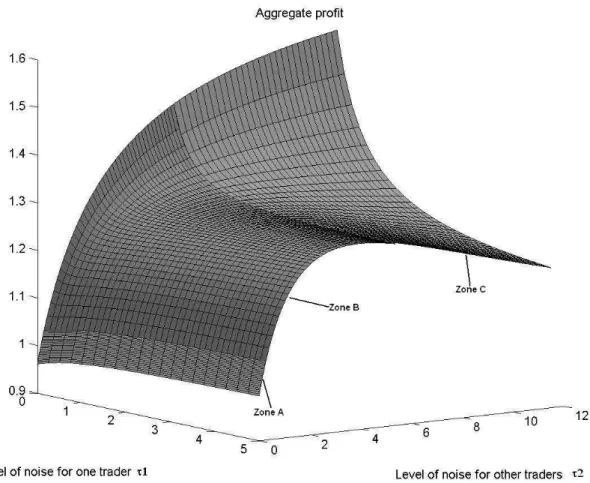
FIGURE 1 GOES HERE
Figure 1 shows the aggregate expected profit of 11 traders in the specific case for which we have one trader with his own level of noise τ1 and ten traders each with the same level of noise τ2. To distinguish the three zones, we have marked each of them with a different mesh.
• Zone A: For small levels of noise in the signals - b(τ−i) ≤ 0 and c(τ−i) ≤ 0 - which is fulfilled here for τ2 between 0 and 0.265, the aggregate expected profit is always increasing with the level of noise of the τ1 trader.
• Zone B: for an amount of noise τ2 in the signals of others which fulfills b(τ−i) ≤ 0 and
c(τ−i) ≥ 0, here for τ2between 0.265 and 5.354, the aggregate expected profit, as a function of τ1, decreases when τ1 ≥ 2b(τc(τ22)) and increases when τ1≤ 2b(τc(τ22)).
• Zone C: for a sufficient level of noise τ2, here with τ2 > 5.354 the aggregate expected profit is always decreasing with the level of noise of the τ1 trader.
These new patterns – namely the non-monotonicity of both liquidity and expected profits – lead us to characterize sets of information for which the presence of heterogeneous noise in signals can generate greater profits than the ones achieved with perfect information.
In our opinion, this result is a key contribution of the paper because it pinpoints the tradeoff between noise and competition. In Holden and Subramanyam (1992) the expected profits de-crease quickly with the number of traders. The traders cannot hide their private information. In Foster and Vishnathan (1996) and Back, Cao and Willard (2000), the initial correlation between the signals determines the kind of competition. If the correlation is positive but not perfect there are two phases over time. First, the rat race, when competition is fierce. Second, the waiting game when traders are on opposite sides of the market. This creates an incentive to wait to trade. Therefore, in this second phase competition becomes less fierce. In our model, since it is a one period game, we have the same effect as in the rat race.
4
The Symmetric Case
We focus in this section on the symmetric heterogeneous signals case, that is the setup when all informed agents are endowed with signals of the same precision, σi = σ1 for i = 1, . . . , N . We still maintain the mutual independence of {eε1, . . . , eεN, ev, eu}. Then we can state the following proposition as a particular case of the previous propositions 3.1 − 3.3.
3.1. In this particular case (β∗ 1, . . . , βN∗, λ∗) (σ1, N ) is characterized by: β∗ i(σ1, N ) = β∗(σ1, N ) = σσu v 1 √ N s 1 +σ21 σ2 v , i = 1, . . . , N, 1 λ∗(σ1, N ) = σu σv N + 1 + 2σ12 σ2 v √ N s 1 +σ12 σ2 v ·
In equilibrium, the individual profit π∗
i(σ1, N ), for i = 1, . . . , N is given by:
π∗i(σ1, N ) = σvσu s 1 +σ12 σ2 v √ N µ N + 1 + 2σ 2 1 σ2 v ¶ , (6)
and the aggregate profit π∗(σ
1, N ) is: π∗(σ1, N ) = σvσu √ N s 1 +σ 2 1 σ2 v N + 1 + 2σ12 σ2 v · (7)
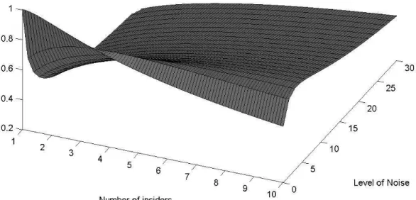
FIGURE 2 GOES HERE
Figure 2 presents the normalized aggregate profit as a function of the level of noise in the signals and the number of insiders. The normalization is performed with respect to the profit achieved by the monopoly in Kyle (1985) setup (π∗(0, 1) = 1
2σuσv).
By setting σ1 = 0, we get the Holden and Subramanyam (1992) and the Admati and Pfleiderer (1986) results, notably that the aggregate profit is close to zero when the number of insiders is large. We provide in the following proposition a detailed characterization of the parameters which determine profits.
Proposition 4.2 i) For a number of informed traders N ≥ 4, individual profits are increasing with the noise in the insider’s information for σ1 smaller than σv
r
N − 3
2 , and individual
profits are maximized at σ∗
1(N ) = σv r
N − 3
2 . This is related to the two effects (beneficial and
costly ones) of the noise in the collection of information.
ii) For a small number of informed traders (N ≤ 3), the aggregate profit is always de-creasing with the level of noise in the signals.
iii)In equilibrium, the informed traders’ aggregate profit evaluated at the optimal level of noise is:
π∗inf ormed traders(N ) = π∗(N ) = σvσu 2√2 1 r 1 − 1 N .
iv) For all N ≥ 4, the insiders make a greater profit than in the perfectly informed case since σ1 is smaller than σv
√
N + 1√N − 3
2 .
Proof See Appendix C.1.
Proposition 4.2 states that for the entire interval (0, BN) with BN = σv
√
N + 1√N − 3
2 , noise
in signals is preferable. Of course, there is a particular value σ∗2
1 (N ) for which the expected profits are maximized. It is important to note that we do not describe how to implement the optimal level of noise. However, we derive all the properties of the model for this optimal value. We do not formally present ways for traders to implement this value in their strategies. For example, traders could collude or put in place contracts for the sale of information as in Admati and Pfleiderer (1986) or Germain (2005).
Moreover, it is important to note that as N increases, the interval for which noise and signals is preferable widens and at the limit extends to the whole positive real line. In this respect, we can argue that the value of information becomes more and more negative as N increases. Moreover, this result relies solely on the heterogeneous signals framework. Indeed, we already know from Admati and Pfleiderer (1988a), that in case of homogeneous signals (i.e. same signals), the value of information does not become more negative as N increases.
FIGURE 3 GOES HERE
Figure 3 shows the individual profit of the informed traders as a function of both the level of noise in the signals and of the number of insiders for more than four insiders. We have plotted in bold the individual profit for the optimal amount of noise as a function of the number of insiders.
The expected aggregate profit π∗(N ) = N π∗i(N ) does not go to zero when N is large, but instead tends to a finite positive value σvσu
2√2. In the literature Admati and Pfleiderer (1988a) have focused on homogeneous signals. In our framework of heterogeneous signals two cases have to be distinguished. When the precision of information is fixed and different from the optimal level of noise, the expected aggregate profits go to zero with the number of informed traders. Otherwise, for the optimal level of noise in signals, the expected aggregate profit goes to a finite
positive limit. In contrast to the Holden and Subramanyam (1992) model, the competition between informed traders may not destroy all their profits. In Foster and Vishnathan (1996) and Back, Cao and Willard (2000) the fierce competition causes almost all private information to be released in the earlier periods and therefore the aggregate expected profit tends to zero; this convergence is faster when the initial correlation between the informed traders’ signals is high.
In Figure 4, the aggregate expected profit is represented as a function of the number of insiders for both the optimal noise and the perfect information. When traders have perfect information, they reveal it immediately, and the aggregate expected profit tends to zero when the number of informed traders is large. However, Figure 4 shows that they can substantially reduce the negative consequences of competition by using an optimal level of noise in their signal.
FIGURE 4 GOES HERE As the liquidity is the inverse of the aggregate profit times σ2
v, one can show that when insiders have perfect information, the liquidity tends to infinity with the number of informed traders. However, at the optimal level of noise the liquidity tends to a finite limit λ−1
∞ =
σu σv
2√2 when the number of insiders is large.
In order to fully understand this result, we need to focus on the informativeness of prices and also on the process of aggregation of the collection of information. This is the purpose of the next proposition.
Proposition 4.3 : For each level of signal precision and number of informed traders (σ1, N ),
the informativeness of prices I(σ1, N ) is given in equilibrium by:
I(σ1, N ) = {V ar (ev|ep)}−1 = {V ar (ev| ew)}−1= σ12 v N + 1 + 2σ12 σ2 v 1 + 2σ 2 1 σ2 v , (8)
The informativeness of prices I∗(N ) for the optimal level of noise in the signals σ∗
1(N ) at
equilibrium is given by:
I∗(N ) = V ar (ev| ew)−1= 1
σ2 v
2(N − 1)
N − 2 , (9)
and when N is large, I∗(N ) is equivalent to:
I∗(N ) = V ar (ev|w)−1 ∼ N →+∞ 2 σ2 v · (10) If we denote S = 1 N N X i=1 Si, then:
• if σ2 1 is fixed, * S −→L2 N →+∞v, * pe L2 −→ N →+∞v • if σ2 1 = σ∗ 2 1 (N ), * S − v −→L N →+∞ σv √ 2X, with X à N (0, 1), * p −e 1 2v L −→ N →+∞ σv 2 Y , with Y = 1 √ 2 µ X + u σu ¶ à N (0, 1), * p − Se −→L N →+∞− 1 2v + √ 3 4 σvZ, with Z = − 1 √ 3X + r 2 3 u σu à N (0, 1)
Proof See Appendix C.2.
Proposition 4.3 shows that the informativeness of prices tends to infinity for a fixed variance of the signals, whereas there is a finite limit for the case of optimal noise in the signals or more generally when the noise in the signals is of the same order as the optimal one. This shows that in the latter case efficiency is not reached in this market. This is confirmed by the results on the aggregation of information. When the variance is fixed, both the statistic S and the price e
p aggregate to the actual value v. For the case of optimal noise in the signals, the statistic S
appears at the limit as the sum of the actual value v plus some error term. Thus, the collection of signals S does not aggregate to the final liquidation value of the risky asset. Nor does the price ep aggregate to the value v. Indeed, it equals 1
2v plus an error term. Moreover, the price ep does not aggregate the statistics S.
This relies on both heterogeneous signals and optimal noise in signals or more generally on noise in signals being of the same order as the optimal noise. In this context, we can understand why at the limit the expected aggregate profits do not go to zero for large N . This is essentially due to the imperfect aggregation of information. As a result, in this economy as the number of competitors becomes larger, the market is not strongly efficient3 With perfect information, the competition between informed traders cancels almost all uncertainty in the market. In this case, the market is strongly efficient as shown in Holden and Subramanyam (1992). However, in Foster and Vishwanathan (1996) as well as in Back, Cao and Willard (2000) competition may or may not lead to greater efficiency of prices. There is more or less uncertainty left depending on how the information is distributed among the agents. Moreover, in their model they show that the market is more efficient when the information is possessed by a single trader than when
3The efficiency of the price in our paper is the same concept as the informativeness of the price which is
measured by the quantity {V ar(ev|ep)}−1. Thus, a strongly efficient price is a price which reveals all the information
several traders share information by means of correlated signals. This result is similar to the result we obtain with the optimal level of noise.
Proposition 4.4 : In equilibrium, the aggregate profit, where π∗(N, σ
1) is maximized for the
value N = N∗(σ 1). N∗(σ 1) = 1 + 2σ 2 1 σ2 v , if 1 + 2σ21 σ2 v is a positive integer, N∗(σ 1) = argmax N ∈( eN1(σ1), eN2(σ1)) π∗(N, σ1), if 1 + 2σ12 σ2 v
is not a positive integer,
(11) and eN1(σ1) = int µ 1 + 2σ 2 1 σ2 v ¶ , e N2(σ1) = eN1(σ1) + 1. Proof : Straightforward.
Proposition 4.4 states that for a given level of available information precision σ1, there exists an optimal size of the market N∗(σ1) for which the aggregate profit is maximized. Moreover, the greater the level of noise in the signals the bigger the market. One implication of this result is that for the case of direct sale of information as in Admati and Pfleiderer (1986-1990), a seller of information should choose N∗(σ
1) participants.4
5
Concluding Remarks
We determine the nature of the competition according to the distribution of information among insiders. Firstly, we show that each insider reacts all the more to her private information as the other informed traders’ information is more noisy. More generally, we point out a tradeoff between the noise and the competition. We show that noise weakens the competition between traders so that they compete less aggressively. We delineate several regions of level of noise which lead to different profiles of liquidity and profits and compute the optimal level of noise. Under certain conditions, we point out regions of level of noises for which the expected profits of the insiders increase in the level of noise and are higher than the ones when insiders know perfectly the liquidation value of the risky asset and expected profits decrease slowly with the number of insiders. This differentiates us from Holden and Subramanyam (1992) where profits decrease quickly with the number of insiders. A possible extension of our model would be to study the tradeoff between noise and competition in a dynamic setting. Boco and Germain (2007) study this dynamic tradeoff in the case of direct sales of information.
A.1. Proof of Proposition 3.1
Agent i maximizes his conditional expected profit (N ≥ 2):
max x∈IRE x ev − λ x +X j6=i e xj+ eu | Si . i = 1, . . . , N, Since eu and eSi are independent, we have:
max x∈IR 1 1 + τiSix − λx 2− λxX j6=i E (exj | Si) , i = 1, . . . , N · It follows that: e xi= 2λ1 1 + τ1 iSi− 1 2 X j6=i E (exj | Si) = 0, i = 1, . . . , N, (12) Let {x∗
i, i = 1, . . . , N } be a particular solution to (12). Then if we define: e
yi = exi− x∗i, i = 1, . . . , N,
{exi, i = 1, . . . , N } is a solution to (12) if and only if {eyi, i = 1, . . . , N } is a solution to (13): e yi = −1 2 X j6=i E (eyj | Si) , i = 1, . . . , N · (13)
We now show that equation (13) has exactly one solution : eyi=0 for i = 1, . . . , N almost surely. Define yei+ 1 2 X j6=i e
yj = eηifor i = 1, . . . , N . From (13) we have that E (eηi/Si) = 0. We consider the linear system:
e y1+ 12 X j6=1 e yj = eη1 .. . e yn+12 X j6=n e yj = eηn By inverting we obtain that
for i = 1, . . . , N, yei = 2 N + 1 N eηi− X j6=i e ηj ·
If we substitute the latter relation into (13), we obtain that ey is a solution to (13) if and only if
there exists {eηi, i = 1, . . . , N } such that E[eηi|Si] = 0 and (1) eyi = N + 12 N eηi− X j6=i e ηj , i = 1, . . . , N, (2) 2 N + 1 N eηi− X j6=i e ηj = − 1 2 X j6=i E 2 N + 1 N eηj− X k6=j e ηk | Si , ⇐⇒ (1) and N eηi− X j6=i e ηj = −12E N X j6=i e ηj− X j6=i X k6=j e ηk/ | Si , ⇐⇒ (1) and N eηi− X j6=i e ηj = −12E N X j6=i e ηj− (N − 1)eηi− (N − 2) X k6=i e ηk/ | Si , ⇐⇒ (1) and N eηi= X j6=i e ηj− E X j6=i e ηj | Si , i = 1, . . . , N, since E[eηi|Si] = 0·
From the last equation, we deduce that E (eηi) = 0, i = 1, . . . , N since E (eηi) = 1 N E {ez − E [ez | Si]} = 0 where ez = X j6=i e ηj. V ar (eηi) = 1 N2 V ar {ez − E [ez | Si]} = 1 N2 E [V ar (ez | Si)] , ≤ 1 N2 V ar (ez) = 1 N2V ar X j6=i e ηj ≤ 1 N2 X j6=i q V ar (eηj) 2 , V ar X j6=i e ηj = X j6=i V ar (eηj) + 2 X j, k 6= i k < j Cov (eηj, eηk) ≤ X j6=i ·q V ar (eηj) ¸2 + +2 X j, k 6= i k < j q V ar (eηj)pV ar (eηk) = X j6=i q V ar (eηj) 2 ·
=⇒ ∀i = 1, . . . , N, V ar (eηi) ≤ µ N − 1 N ¶2 max j=1,...,N{V ar (eηj)} , =⇒ max i=1,...,NV ar (eηi) ≤ µ N − 1 N ¶2 max j=1,...,N{V ar (eηj)} , =⇒ " 1 − µ 1 − 1 N ¶2# max i=1,...,NV ar (eηi) ≤ 0, =⇒ max i=1,...,NV ar (eηi) = 0· Thus we have for i = 1, . . . , N :
E (eηi) = 0, V ar (eηi) = 0, =⇒ eηi a.s. = 0· Therefore the only solution to (13) is ey = 0 ∈ IRN.
We now show the existence of a linear equilibrium {x∗
i, i = 1, . . . , N } which is, in addition, the unique linear equilibrium. We thus look for a particular solution to (13) of the form
{x∗i = βi∗Si, i = 1, . . . , N }. We introduce the following quantities:
ai= 1 + τ1
i < 1, i = 1, . . . , N,
bi = 1 2λai·
Thanks to the normality assumption and the mutual independence of {ev, eε1, . . . , eεN}, we have
E
³ e
Sj | Si ´
= aiSi for j 6= i. Using (12), we have
βiSi = biSi−12 X j6=i E h βjSej | Si i = biSi−12 X j6=i aiβjSej, i = 1, . . . , N, or equivalently βi= bi−ai 2 X j6=i βj, i = 1, . . . , N, βi µ 1 2 + τi ¶ = 1 2λ− 1 2 N X j=1 βj, i = 1, . . . , N, βi= 1 + 2τa i ⇐⇒ 1 λ= a 1 + N X j=1 1 1 + 2τj , (14)
with a independent of i. We also know that, at equilibrium, ep = E (ev|w). In this particular
equilibrium, we have ew =
N X
i=1
normality of each components, it follows that ep = λw and that therefore we obtain a linear equilibrium with λ = Cov (ev, ew) V ar ( ew) = Cov ev,XN j=1 βjSej + eu V ar XN j=1 βjSej+ eu = N X j=1 βjσ2v XN j=1 βj 2 σ2 v+ N X j=1 βj2σ2j + σ2u , so 1 λ= a N X j=1 1 1 + 2τj + a N X j=1 τj 1 (1 + 2τj)2 N X j=1 1 1 + 2τj +σu2 σ2 v 1 a N X j=1 1 1 + 2τj · (15)
Using (14) and (15), we obtain:
a 1 − N X j=1 τj (1 + 2τj)2 N X j=1 1 1 + 2τj = σu2 σ2 v 1 a N X j=1 1 1 + 2τj , so that a = σu σv 1 N X j=1 1 + τj (1 + 2τj)2 1 2 ,
Inserting the above value of a into (12) yields the formula for β∗
i(σ) and 1
λ∗(σ) in the proposition. Following algebraic manipulation, we obtain the formula of the expected individual profit at the equilibrium: π∗ i(σ) = σvσu 1 +XN j=1 1 1 + 2τj N X j=1 1 + τj (1 + 2τj)2 1 2 1 + τi [1 + 2τi]2 ·
This ends the proof of Proposition 3.1. B.1. Proof of proposition 3.2
We calculate the derivative of β∗
i with respect to τj and then with respect to τi. After simplification, we obtain ∂β∗ i ∂τj (τ ) = 1 2 σu σv 3 + 2τj N X j=1 1 + τj (1 + 2τj)2 3 2 (1 + 2τi) (1 + 2τj)3 > 0, for j 6= i, so ∂β∗ i ∂τi(τ ) = − 1 2 σu σv 4 (1 + 2τi)X j6=i 1 + τj (1 + 2τj)2 + 1 N X j=1 1 + τj (1 + 2τj)2 3 2 (1 + 2τi)3 < 0·
We do the same with the function ln(π∗ i(τ )) ∂ ln πi∗ ∂τj (τ ) = 1 2 3 + 2τj N X k=1 1 + τk (1 + 2τk)2 (1 + 2τj)3 +" 2 1 + N X k=1 1 1 + 2τk # (1 + 2τj)2 > 0
=⇒ πi∗(σ) is increasing in σ−i, theref ore
∂ ln πi∗ ∂τi (τ ) = 1 2 3 + 2τi (1 + 2τi)3 N X k=1 1 + τk (1 + 2τk)2 + 2 (1 + 2τi)2 " 1 + N X k=1 1 1 + 2τk # + 1 1 + τi − 4 1 + 2τi, = 1 2 (1 + 2τi)3 " N X k=1 1 + τk (1 + 2τk)2 # " 1 + N X k=1 1 1 + 2τk # (1 + τi) gi(τ ), where gi(τ ) = (3 + 2τi) (1 + τi) " 1 + N X k=1 1 1 + 2τk # + 4 (1 + 2τi) "N X k=1 1 + τk (1 + 2τk)2 # (1 + τi) −2 (3 + 2τi) (1 + 2τi)2 N X k=1 1 + τk (1 + 2τk)2 " 1 + N X k=1 1 1 + 2τk # . The sign of ∂ ln π ∗ i
−2 (1 + τi)2− (3 + 2τi) (1 + τi) X k6=i 1 1 + 2τk − 8 (1 + 2τi) (1 + τi) 2X k6=i 1 + τk (1 + 2τk)2 −2 (3 + 2τi) (1 + 2τi)2 X k6=i 1 + τk (1 + 2τk)2 X k6=i 1 1 + 2τk· Since gi(τ ) < 0 it follows that πi∗(σ) is decreasing in τi= σ
2 i
σ2 v . This ends the proof of Proposition 3.2.
B.2. Proof of Proposition 3.3 ∂λ∗−1 ∂τi (τ ) = σu σv 1 2 (3 + 2τi) 1 +XN j=1 1 1 + 2τj N X j=1 1 + τj (1 + 2τj)2 3 2 (1 + 2τi)3 − 2 N X j=1 1 + τj (1 + 2τj)2 1 2 (1 + 2τi)2 , ∂λ∗−1 ∂τi (τ ) = 1 2 σu σv 1 N X j=1 1 + τj (1 + 2τj)2 3 2 (1 + 2τi)3
hi(τ ), with : hi(τ ) = 2τib(τ−i) + c(τ−i),
where b(τ−i) and c(τ−i) are defined in Proposition (3.3). It is worth noting that c(τ−i) > b(τ−i), indeed c(τ−i) − b(τ−i) = 1 +
X j6=i
2
1 + 2τj. This ends the proof of Proposition 3.3. If we define ΣN as
ΣN = {σ = (σ1, . . . , σN)0∈ IRN+ | ∀i = 1, . . . , N π∗i(σ1, . . . , σN) ≥ πi∗(0, . . . , 0),
and ∃i◦∈ (1, . . . , N ) with πi∗◦(σ1, . . . , σN) > π
∗
i◦(0, . . . , 0)},
we have
• for N ≥ 4 ΣN is non-empty. In other words, noise in the collection of signals is ex–ante optimal;
• for N ≤ 3, ΣN is empty.
In order to show the result of the non-emptiness of ΣN for N ≥ 4, we just need to focus on the symmetric case where σ1 = . . . = σN and this is the purpose of proposition 4.2. We now show that ΣN is empty for N ≤ 3.
Proof for N=2:
(As the proofs for N=2 and N=3 are almost identical, we leave this proof to the reader.) Proof for N=3: πi(τ ) = σuσv 1 + τi (1 + 2τi)2 3 X j=1 1 + τj (1 + 2τj)2 1 2( 1 + 3 X i=1 1 1 + 2τi )· We again denote xi = (1 + 2τ1 + τi i)2, i = 1, 2, 3. For τi 6= 0, xi < 1, yi = 1 1 + 2τi = √ 1 + 8xi− 1 2 .
Therefore, for i = 1, 2, 3 we have
πi(τ ) = σvσu 2xi X3 j=1 xj 1 2 X3 j=1 p 1 + 8xj− 1 , πi(0) = σvσu 4√3·
We already know that for τ1 = τ2 = τ3 6= 0, π1(τ ), π2(τ ) and π3(τ ) are strictly smaller than
πi(0) = σvσu
4√3 and equal if and only if τ1 = τ2 = τ3 = 0. We thus focus on cases where
∃ (i, j) ∈ {1, 2, 3}2 such that τj 6= τi ⇐⇒ xj 6= xi. Without any loss of generality, we will suppose (up to a reordering) that:
a) either x1 > x2 ≥ x3,
b) or x1≥ x2 > x3.
Now assume that πi(τ ) ≥ σvσu
4√3, i = 1, 2, 3. a)If x1> x2≥ x3: then x3≥ 1 8√3 3 X j=1 xj 1 2 3 X j=1 p 1 + 8xj− 1 =⇒ 8√x3≥ 3 √ 1 + 8x3− 1·
Let f be:
f (x) = 8√x − 3√1 + 8x + 1,
where 0 ≤ x, so
f0(x) = √ 4(1 − x)
x√1 + 8x£√1 + 8x + 3√x¤ ·
f is increasing on [0, 1], decreasing on [1, +∞[ and f (1) = 0. Therefore ∀x ≥ 0, f (x) ≤ 0 and f (x) = 0 =⇒ x = 1.
8√x3 ≥ 3
√
1 + 8x3− 1 =⇒ x3 = 1, which is ruled out.
b) x1≥ x2> x3: the proof is analogous. The above cases imply that Σ3 is empty. C.1. Proof of Proposition 4.2 N ≥ 4, π∗ i(σ1) > πi∗(0), ⇐⇒ √ 1 + τ √ N (N + 1 + 2τ ) > 1 √ N (N + 1), where τ = σ2 1 σ2 v > 0 ⇐⇒ σ1 < σ2v √ N − 3√N + 1· π∗ i(τ ) = σvσu √ 1 + τ √ N (N + 1 + 2τ ), ∂ ln π∗ i ∂τ (τ ) = ∂ ∂τ ½ 1 2ln (1 + τ ) − ln (N + 1 + 2τ ) ¾ , = 1 2 (1 + τ ) − 2 N + 1 + 2τ = N − 3 − 2τ 2 (1 + τ ) (N + 1 + 2τ )· Therefore π∗ i(τ ) is maximized for τ = N − 3
2 . This ends the proof of Proposition 4.2. C.2. Proof of Proposition 4.3
ev e w à N 0 0 , σ2v √ N σuσv s 1 +σ21 σ2 v √ N σuσv s 1 +σ12 σ2 v σ2 u 1 +N + σ2 1 σ2 v 1 +σ21 σ2 v , ev e u is normal =⇒ ev e w
is normal. Moreover, we have:
• Cov (ev, ew) = Cov à e v, N β∗(σ1, N )ev + N X i=1 β∗(σ1, N )eεi+ eu ! = N β∗(σ1, N )σ2v = √ N σuσv q 1 +σ12 σ2 v · • V ar ( ew) = V ar à N β∗(σ1, N )ev + N X i=1 β∗(σ1, N )eεi+ eu ! = N2β∗2(σ1, N )σv2+ N β∗ 2 (σ1, N )σ12+ σu2, V ar ( ew) = N σ2u 1 +σ21 σ2 v + σ 2 uσ 2 1 σ2 v 1 +σ12 σ2 v + σu2 = σu2 1 + N + σ2 1 σ2 v 1 +σ21 σ2 v , • V ar (ev | w) = V ar (ev) − [Cov (ev, ew)] 2 V ar ( ew) = σ 2 v 1 − N N + 1 + 2σ12 σ2 v ·
Fig. 1. Aggregate profit of the traders as a function of both the level of noise in the signal of one trader and the level of noise in the signal of the other traders.
Figure 1:
This figure shows the aggregate expected profit of 11 traders in the specific case for which we have on the one hand a trader with his own level of noise τ1 and on the other hand 10 traders with the same level of noise τ2.
Fig. 2. Normalized aggregate profit as a function of both the level of noise in the signals and the number of insiders.
Figure 2: This figure represents the normalized aggregate profit as a function of the level of noise in the signals and the number of insiders. The normalization is performed with respect to the profit achieved by the monopoly in Kyle’s (1985) setup (π∗(0, 1) = 1
Fig. 3. Individual profit as a function of both level of noise in the signals and the numbers of insiders with a number of insiders higher than 4.
Figure 3: This figure shows the individual profit of the informed traders as a function of both the level of noise in the signals and the number of insiders for more than four insiders. We have plotted in bold the optimal amount of noise as a function of the number of insiders.
Fig. 4. Aggregate profit: Optimal symmetric noise versus perfect information.
Figure 4: This figure shows the aggregate profit as a function of the number of insiders for both the optimal noise and the perfect information cases.
References
Admati, A., and Pfleiderer, P., 1986. A Monopolistic Market for Information. J. Econ. Theory, 39, 400-38.
Admati, A., and Pfleiderer, P., 1988a. Selling and Trading on Information in Financial Markets, American Econ. Rev., 78, 1165-1183.
Admati, A., and Pfleiderer, P., 1988b. A Theory of Intraday Patterns: Volume and Price Variability. Rev. Finan. Stud, 1, 3-40.
Admati, A., and Pfleiderer, P., 1990. Direct and Indirect Sale of Information. Econometrica 58, 901-928.
Back, K., Cao, K., and Willard, A., 2000. Imperfect Competition Among Informed Traders. J. Finance 5, 2117-2155.
Biais, B., and Germain, L., 2002. Incentive Compatible Contracts for the Sale of Information. Rev. Finan. Stud 4, 987-1004.
Biais, B., Martimort, D., and Rochet, J. C., 2000. Competing Mechanisms in a Common Value Environment. Econometrica 4, 799-837.
Boco, H., and Germain, L., 2007 Optimal Market Size for Selling on Information. forthcoming. Foster, F. D., and Viswanathan, S., 1994. Strategic Trading with Asymmetrically Informed
Traders and Long-lived Information. J. Fin. and Quant., 29, 499-518.
Foster, F. D., and Viswanathan, S. 1996. Strategic Trading When Agents Forecast the Forecasts of Others. J. Finance 51, 1437-78.
Germain, L., 2007. Strategic Noise in Competitive Markets for the Sale of Information. forth-coming J. Finan. Intermediation.
Grossman, S. J., 1976. On the Efficiency of Competitive Stock Markets Where Traders Have Diverse Information. J. Finance 31, 573-585.
Grossman, S. J., and Stiglitz, J. E., 1980. On the Impossibility of Informationally Efficient Markets. American Econ. Rev 70, 393-408.
Hellwig, M. F., 1980. On the Aggregation of Information in Competitive Markets. J. Econ. Theory 22, 477-498.
Holden, C. W., and Subrahmanyam, A., 1992. Long-Lived Private Information and Imperfect Competition. J. Finance 47, 247-270.
Holden, C. W., and Subrahmanyam, A., 1994. Risk Aversion, Imperfect Competition and Long-lived Information. Econ. Letters 44, 181-190.
Kyle, A., 1984. Market Structure, Information, Futures Markets and Price Formation in In-ternational Agricultural Trade. Advanced Readings in Price formation, Market Structure,
and Price Instability ed. Story, Schmitz and Sarris (Westview Press, Boulder and London).
Kyle, A., 1985. Continuous Auctions and Insider Trading. Econometrica 53, 1315-1335. Rochet, J. C., and Villa, J. L., 1994. Insider Trading without Normality. Rev. Econ. Stud 61,