Thermochemical non-equilibrium effects in turbulent ... - SAM

Science Arts & Métiers (SAM)

is an open access repository that collects the work of Arts et Métiers Institute of Technology researchers and makes it freely available over the web where possible.

This is an author-deposited version published in: https://sam.ensam.eu Handle ID: .http://hdl.handle.net/10985/21900

To cite this version :

Donatella PASSIATORE, Luca SCIACOVELLI, Paola CINNELLA, Pascazio GIUSEPPE -

Thermochemical non-equilibrium effects in turbulent hypersonic boundary layers - Journal of Fluid Mechanics - 2022

Any correspondence concerning this service should be sent to the repository Administrator : [email protected]

Thermochemical non-equilibrium effects in turbulent hypersonic boundary layers

D. Passiatore^1,2,†, L. Sciacovelli², P. Cinnella³and G. Pascazio¹

1Politecnico di Bari, DMMM, via Re David 200, 70125 Bari, Italy

2DynFluid Laboratory, Arts et Métiers Institute of Technology, 151 bd. de l’Hôpital, 75013 Paris, France

3Sorbonne Université, Institut Jean Le Rond d’Alembert, 4 Place Jussieu, 75005 Paris, France

A hypersonic, spatially evolving turbulent boundary layer at Mach 12.48 with a cooled wall is analysed by means of direct numerical simulations. At the selected conditions, massive kinetic-to-internal energy conversion triggers thermal and chemical non-equilibrium phenomena. Air is assumed to behave as a five-species reacting mixture, and a two-temperature model is adopted to account for vibrational non-equilibrium. Wall cooling partly counteracts the effects of friction heating, and the temperature rise in the boundary layer excites vibrational energy modes while inducing mild chemical dissociation of oxygen. Vibrational non-equilibrium is mostly driven by molecular nitrogen, characterized by slower relaxation rates than the other molecules in the mixture. The results reveal that thermal non-equilibrium is sustained by turbulent mixing: sweep and ejection events efficiently redistribute the gas, contributing to the generation of a vibrationally under-excited state close to the wall, and an over-excited state in the outer region of the boundary layer. The tight coupling between turbulence and thermal effects is quantified by defining an interaction indicator. A modelling strategy for the vibrational energy turbulent flux is proposed, based on the definition of a vibrational turbulent Prandtl number. The validity of the strong Reynolds analogy under thermal non-equilibrium is also evaluated.

Strong compressibility effects promote the translational–vibrational energy exchange, but no preferential correlation was detected between expansions/compressions and vibrational over-/under-excitation, as opposed to what has been observed for unconfined turbulent configurations.

Key words:compressible boundary layers, hypersonic flow, turbulent reacting flows

†Emailaddressforcorrespondence:[email protected]

1. Introduction

High-speed flows represent a challenging topic of interest for manifold configurations, including objects entering a planetary atmosphere or for atmospheric hypersonic flight (Gnoffo et al. 1999). In such flows, conversion of massive amounts of kinetic energy into internal energy causes a sudden rise of the flow temperature. The effects triggered by the high temperatures include chemical reactions and vibrational relaxation phenomena on characteristic time scales comparable to the flow time scales. The complex thermochemical state induced by such conditions may affect quantities of interest for the design of high-speed vehicles significantly (Bertin & Cummings2006; Candler2019). In the past, thermochemical effects caused by hypersonic conditions have been investigated in more or less simple configurations. Most of the efforts focused on stagnation-point flows, of interest for bluff bodies re-entering the atmosphere (Fay & Riddell1958; Armenise et al. 1996; Bonelli et al. 2017; Colonna, Bonelli & Pascazio 2019). In later stages of re-entry trajectories or for suborbital flight conditions characterized by higher free-stream densities, the flow description is further complicated by the transition from a laminar to a turbulent regime. Such a transition may be triggered by free-stream disturbances, erosion and ablation of the thermal protection systems (TPS) or due to surface defects, leading to sharp rise of the skin friction and heat fluxes at the walls. For this reasons, laminar-to-turbulent transition has been identified as a subject of major concern for the accurate prediction of the aerothermodynamic flow fields around objects flying at hypersonic speeds. A significant number of contributions in the literature have addressed the linear and nonlinear stability of flat-plate boundary layers in chemical non-equilibrium, sometimes up to the initial stages of transition. The pioneering studies of Malik &

Anderson (1991), Hudson, Chokani & Candler (1997) and Perraudet al.(1999) pointed out that chemical reactions tend to promote the so-called second mode instability, similarly to strongly cooled walls. More recently, Marxenet al.(2013) and Marxen, Iaccarino & Magin (2014) used direct numerical simulations (DNS) to evaluate the maximum streamwise velocity disturbance caused by large- or small-amplitude waves in presence of chemical reactions. Kline, Chang & Li (2019) and Knisely & Zhong (2019) investigated the effects of thermochemical non-equilibrium (TCNE) on boundary-layer stability; the effect of ablation has also been considered (Mortensen & Zhong2016; Miró Miró & Pinna2021).

On the other hand, while wall-bounded turbulence under low-enthalpy conditions (i.e. with air behaving as a calorically perfect gas) has been carefully scrutinized over the years, the interplay between TCNE conditions and turbulence has received much less attention.

Compressible turbulent boundary-layer (TBL) configurations have been investigated with different turbulence injection techniques and wall treatments; for a thorough overview of DNS of TBLs at relatively low free-stream Mach numbers (M_∞ ≤3), the reader may refer to the work of Wenzelet al.(2018) and references therein. Many efforts have been devoted to extending the validity of scaling laws derived for incompressible configurations (Morkovin 1962) to compressible ones. Inspection of the hypersonic regime by means of high-fidelity simulations was initiated by the studies of Duan, Beekman & Martín (2011), who performed DNS of temporally evolving TBLs with nominal free-stream Mach numbers up to 12 to prove the robustness of Morkovin’s hypothesis even in high-speed flows. A DNS of a transitional spatially evolving boundary layer at Mach 6 was performed by Franko & Lele (2013), whereas Zhang, Duan & Choudhari (2018) produced a database of cooled boundary layers up toM_∞=14, with flow conditions representative of those encountered in hypervelocity wind tunnels. Huang et al. (2020) performed DNSs of zero-pressure-gradient hypersonic TBLs and conducteda priorianda posteriorianalyses of the performances of different Reynolds-averaged Navier–Stokes (RANS) models. A

handful of works focused on high-enthalpy flows, at free-stream conditions for which dissociation and recombination reactions are triggered (Martin & Candler2001; Duan &

Martín2009). A comparative study between low- and high-enthalpy, reactive, temporally evolving boundary layers was performed by Duan & Martín (2011b); the authors found that the two closely resemble each other, since the scaling laws validated under low-enthalpy conditions still hold or could be generalized for high-enthalpy applications. The interaction of finite-rate chemistry with transitional and turbulent spatially developing boundary layers was recently investigated by Passiatore et al.(2021) and Di Renzo & Urzay (2021), who isolated the effects of chemical non-equilibrium on pseudo-adiabatic and cooled TBLs, respectively. In both studies, the effect of thermal non-equilibrium was neglected since the selected edge conditions were not expected to promote significant vibrational relaxation phenomena. The influence of these processes on turbulent flow behaviour has been investigated only for unconfined flow configurations so far, such as isotropic turbulence decay (Nevilleet al.2014; Khurshid & Donzis2019; Zhenget al.2020) and mixing layers (Nevilleet al.2015; Fiévetet al.2019).

The present work aims at bridging this knowledge gap with the investigation of a TBL exposed to both thermal and chemical non-equilibrium conditions. For that purpose, we perform a DNS of a flat-plate boundary layer, subjected to post-shock conditions of a 6^◦ sharp wedge flying at Mach 20. The edge thermodynamic state is such that vibrational relaxation phenomena are significant within the boundary layer, while a mild chemical activity is developed.

The paper is organized as follows. The governing equations, the numerical method, the outline of the simulation and the main parameters are described in §2. Numerical results are presented in §3; focusing mostly on the fully turbulent regime, we illustrate the behaviour of the dynamic field and compare different transformations for the streamwise velocity. Afterwards, thermal non-equilibrium effects are inspected by highlighting the tight coupling with turbulent mixing mechanisms. Correlations deriving from the strong Reynolds analogy are also evaluated, as well as classical closures of the new terms arising in the RANS equations. Lastly, the coupling between compressibility effects and thermal non-equilibrium is investigated. Conclusions are then drawn in §4.

2. Methodology

2.1. Governing equations and thermodynamic models

The fluid under investigation in the current study is air at high temperature, modelled as a five-species mixture of N2, O2, NO, O and N. When considering a gas under thermal non-equilibrium conditions, the vibrational energetic levels of the molecules in the mixture are partially excited and no longer equilibrated with the roto-translational ones. A direct consequence is that, even assuming that particle populations follow a Boltzmann distribution, the utilization of a single static temperature to represent all the energetic modes is no longer valid (Anderson 2006). A classical approach to deal with such conditions, referred to as multi-temperature in the literature, consists of taking into account the vibrational levels separately, by means of additional ‘vibrational’ temperatures for each molecule. In order to keep a reasonable number of equations to be integrated, the two-temperature model of Park (1988) is adopted for the present calculations. Such a model, widely used in previous works (see, e.g. Hudsonet al.1997; Franko, MacCormack

& Lele 2010; Bitter & Shepherd 2015), assumes that the vibrational energy states of each molecule satisfy a Boltzmann distribution characterized by only one vibrational temperatureT_V, common to all diatomic species in the mixture (that is, N2, O2 and NO).

A single additional conservation equation is, therefore, needed for the total vibrational energy e_V. Thus, the behaviour of such flows is governed by the compressible Navier–Stokes equations for multicomponent chemically reacting and thermally relaxing gases, which read

∂ρ

∂t +∂ρu_j

∂x_j =0 (2.1)

∂ρu_i

∂t +∂

ρu_iu_j+pδij

∂x_j = ∂τij

∂x_j (2.2)

∂ρE

∂t +∂

(ρE+p)u_j

∂x_j = ∂(u_iτij)

∂x_j −∂(q^TR_j +q^V_j )

∂x_j − ∂

∂x_{j NS}

n=1

ρnu^D_njh_n

(2.3)

∂ρn

∂t +∂ ρnu_j

∂x_j = −∂ρnu^D_nj

∂x_j + ˙ωn (n=1, ..,NS−1) (2.4)

∂ρe_V

∂t +∂ρe_Vu_j

∂x_j = ∂

∂x_j

−q^V_j − NM m=1

ρmu^D_mje_Vm

+ NM m=1

(Q_TVm+ ˙ωme_Vm) . (2.5) In the preceding formulation,ρ is the mixture density,t the time coordinate,x_j the space coordinate in thejth direction of a Cartesian coordinate system, withu_jthe velocity vector component in the same direction,pis the pressure,δij the Kronecker symbol and τij the viscous stress tensor, modelled as

τij=μ ∂u_i

∂x_j +∂u_j

∂x_i

−2 3μ∂u_k

∂x_kδij, (2.6)

withμthe mixture dynamic viscosity. In (2.3),E=e+¹₂u_iu_iis the specific total energy (with e the mixture internal energy), q^TR_j and q^V_j the roto-translational and vibrational contributions to the heat flux, respectively; u^D_nj denotes the diffusion velocity and h_n the specific enthalpy for the nth species. In the species conservation equations (2.4), ρn =ρY_n represents thenth species partial density (Yn being the mass fraction) andω˙n

the rate of production of thenth species. The sum of the partial densities is equal to the mixture densityρ=NS

n=1ρn,NSbeing the total number of species. To ensure total mass conservation, the mixture density andNS−1 species conservation equations are solved, while the partial density of the NSth species is computed as ρNS =ρ−NS−1

n=1 ρn. In the following, we set such species as molecular nitrogen, since it is the most abundant one throughout the computational domain. In (2.5),e_V represents the mixture vibrational energy, given by

e_V = NM m=1

Y_me_Vm, (2.7)

withe_Vm the vibrational energy of the mth molecule andNM their total number. In the same equation,Q_TV =_NM

m=1Q_TVm represents the energy exchange between vibrational and translational modes (due to molecular collisions and linked to energy relaxation phenomena) and NM

m=1ω˙me_Vm the vibrational energy lost or gained due to molecular depletion or production.

Each species is assumed to behave as a thermally perfect gas; Dalton’s pressure mixing law leads then to the thermal equation of state

p=ρT NS n=1

RY_n Mn =T

NS n=1

ρnR_n, (2.8)

withR_n andMnthe gas constant and molecular weight of the nth species, respectively, andR=8.314 J mol⁻¹K⁻¹the universal gas constant. The thermodynamic properties of high-T air species are computed considering the contributions of translational, rotational and vibrational modes; specifically, the internal energy reads

e= NS n=1

Y_nh_n− p

ρ, with h_n=h⁰_f,n+ _T

T_ref(c^T_p,n+c^R_p,n)dT+e_Vn. (2.9) Here, h⁰_f,n is thenth species enthalpy of formation at the reference temperature (Tref = 298.15 K),c^T_p,nandc^R_p,n the translational and rotational contributions to the isobaric heat capacity of thenth species, computed as

c^T_p,n= 5

2R_n and c^R_p,n=

R_n for diatomic species

0 for monoatomic species (2.10a,b) ande_Vnthe vibrational energy of speciesn, given by

e_Vn=

⎧⎨

⎩

θnR_n

exp(θn/T_V)−1 for diatomic species

0 for monoatomic species

(2.11) with θn the characteristic vibrational temperature of each molecule (3393 K, 2273 K and 2739 K for N2, O2 and NO, respectively). After the numerical integration of the conservation equations, the roto-translational temperatureTis computed from the specific internal energy (devoid of the vibrational contribution) directly, whereas an iterative Newton–Raphson method is used to computeT_V from (2.7).

The heat fluxes are modelled by means of Fourier’s law, q^TR_j = −λTR(∂T/∂x_j) and q^V_j = −λV(∂T_V/∂x_j), λTR and λV being the roto-translational and vibrational thermal conductivities, respectively. Pure species’ viscosity and thermal conductivities are computed using curve fits by Blottner, Johnson & Ellis (1971) and Eucken’s relations, respectively (Hirschfelder & Curtiss 1969). The corresponding mixture properties are evaluated by means of Wilke’s mixing rules (Wilke 1950). Mass diffusion is modelled by means of Fick’s law

ρnu^D_nj = −ρD_n∂Y_n

∂x_j +ρn

NS n=1

D_n∂Y_n

∂x_j, (2.12)

where the first term on the right-hand side represents the effective diffusion velocity and the second one is a mass corrector term that should be taken into account in order to satisfy the continuity equation when dealing with non-constant species diffusion coefficients (Poinsot & Veynante 2005). Specifically, D_n is an equivalent diffusion coefficient of speciesninto the mixture, computed following Hirschfelder’s approximation (Hirschfelder

& Curtiss1969), starting from the binary diffusion coefficients which are curve fitted in Guptaet al.(1990). Note that the molecular weight gradient contribution is neglected in (2.12), which therefore represents a rather simple model (albeit allowing for variable mass diffusion coefficients and non-constant Lewis numbers). The five species interact with each other through a reaction mechanism consisting of five reversible chemical steps (Park 1990)

R1 : N2+M⇐⇒2N+M R2 : O2+M⇐⇒2O+M R3 : NO+M⇐⇒N+O+M R4 : N2+O⇐⇒NO+N R5 : NO+O⇐⇒N+O2,

⎫⎪

⎪⎪

⎪⎪

⎪⎬

⎪⎪

⎪⎪

⎪⎪

⎭

(2.13)

with M being the third body (any of the five species considered). Dissociation and recombination processes are described by reactions R1, R2 and R3, whereas the shuffle reactions R4 and R5 represent rearrangement processes. The mass rate of production of thenth species is governed by the law of mass action

˙

ωn =Mn

NR r=1

νnr −νnr

×

k_f,r NS n=1

ρY_n Mn

_νnr

−k_b,r NS n=1

ρY_n Mn

_νnr

, (2.14) where νnr and νnr are the stoichiometric coefficients for reactants and products in the rth reaction for the nth species, respectively, and NR is the total number of reactions.

Furthermore,k_f,r andk_b,r denote the forward and backward reaction rates of reactionr, modelled by means of Arrhenius’ law. The tight coupling between chemical and thermal non-equilibrium, due to their concurrent presence in such flows, is taken into account by means of a suitable modification of the temperature values used for computing the reaction rates. A geometric-averaged temperature is considered for the dissociation reactions R1, R2 and R3 in (2.13), computed asT_avg=T^qT_V^1−qwithq=0.7 (Park1988).

Lastly, the vibrational–translational energy exchange is computed as Q_TV=

NM m=1

Q_TV,m= NM m=1

ρm

e_Vm(T)−e_Vm(T_V)

t_m , (2.15)

wheret_m is themth molecular relaxation time evaluated by means of the expression of Millikan & White (1963). Specifically, the relaxation time of themth molecule with respect to thenth species writes

t_mn^MW = p p_atmexp

a_mn(T^−(1/3)−b_mn)−18.42

, (2.16)

where p is the pressure, p_atm=101 325 Pa and a_mn and b_mn are coefficients reported in Park (1993). Since this expression tends to underestimate the experimental data at temperatures above 5000 K, a high-temperature correction was proposed by Park (1989)

t_mn=t^MW_mn +t^c_mn witht^c_mn=

φmn

Mmσ. (2.17)

Here, φmn=MmMn/(Mm+Mn) and σ =

8R/Tπ(7.5×10⁻¹²NA/T), NA being Avogadro’s number. The mean value is then evaluated with a weighted harmonic average

t_m= NS n=1

ρn

Mn

NS n=1

t_mn

ρn/Mn. (2.18)

The complete formulation of transport coefficients laws and thermochemical models is provided inAppendix A.

2.2. Numerical method

The Navier–Stokes equations are integrated numerically by using a high-order centred finite-difference scheme (Sciacovelli et al.2021). The convective fluxes are discretized by means of central tenth-order differences, supplemented with a higher-order adaptive artificial dissipation. This consists in a blend of a nineth-order accurate dissipation term based on tenth-order derivatives of the conservative variables (used to damp grid-to-grid oscillations) along with a low-order shock-capturing term. A highly selective sensor, based on Ducros’ extension of Jameson’s pressure-based sensor (Ducros et al. 1999) is used to turn on shock capturing in the immediate vicinity of flow discontinuities for all equations except the vibrational energy equation. For the latter, a shock sensor based on second-order derivatives of the vibrational temperature was preferred to ensure appropriate damping of spurious oscillations. Standard fourth-order differences are used for the viscous fluxes. Time integration is carried out by means of a third-order total variation diminishing (TVD) Runge–Kutta scheme (Gottlieb

& Shu 1998). More details about the present numerical technique, as well as a complete assessment for a variety of highly compressible flow problems including chemically reacting hypersonic boundary layers can be found in Sciacovelli et al.

(2021).

2.3. Computational set-up

The configuration under investigation is a spatially evolving, zero-pressure-gradient flat-plate boundary layer, sketched in figure 1. The prescribed edge conditions ofM_e = 12.48,T_e =594.3 K andp_e =4656 Pa are representative of those downstream of a shock wave generated by a 6^◦ sharp wedge flying at M =20 at an altitude of approximately 36 km. The stagnation enthalpy at the edge of the boundary layer is H_e =h_e+u²_e/2= 18.66 MJ kg⁻¹, a value comparable to those of the high-enthalpy cases considered by Duan & Martín (2011b) and Di Renzo & Urzay (2021). Air at such free-stream conditions is supposed to be in thermochemical equilibrium (XN₂=0.79, X_O2=0.21, X_n being the nth species molar fraction). Of note, a similar scenario has been considered by Kline et al. (2019) for stability studies. The computational domain is a rectangular box enclosed within the shock layer, highlighted in red infigure 1. The extent of the domain is L_x×L_y×L_z=3000δ_in ×120δ_in×30πδ_in, withx, y and z denoting the streamwise, wall-normal and spanwise directions, respectively, andδ_in the displacement thickness of the boundary layer at the inlet section, computed as δ=_δ

0(1−ρu/ρeu_e)dy (δ being the boundary-layer thickness at 99 % of the edge velocity). The computational grid is N_x×N_y×N_z=9660×480×512, for a total of approximately 2.4 billions grid points.

The grid spacing is uniform in the streamwise and spanwise directions, whereas a constant grid stretching of 0.7 % is applied in the wall-normal direction. The calculation is initiated in the laminar region at a distance x₀ from the plate leading edge. The profiles of

M_∞ = 20, Re_u = 3.26 × 10⁶ m⁻¹ Air at ≈ 36 km

M_e = 12.48 T_e = 594.3 K, p_e = 4656 Pa

X_N2 = 0.79, X_O2 = 0.21

Non-catalytic, isothermal wall at T = T_V = 1800 K 6^°

Shock wave

S&B LAMINAR TRANSITIONAL

TURBULENT

x₀ = 0.027 m Re_δin = 6054

Re_δforc = 10⁴

Figure 1. Sketch of the configuration under investigation.

the conservative variables prescribed at the inflow are generated by solving the locally self-similar theory for a two-dimensional chemically out-of-equilibrium and vibrationally equilibrated boundary layer (Sciacovelliet al.2021); the inflow Reynolds number based on the inlet displacement thickness isRe_δ

in =6054. Using a thermal equilibrium simplifies the numerical setting and is not expected to alter the qualitative behaviour of the turbulent zone, of interest in the following analyses. A sponge layer is applied downstream of the inlet boundary, up to(x−x₀)/δ_in =20, to prevent abrupt distortions of the boundary layer.

Characteristic-based boundary conditions are imposed at the top and right boundaries, and periodic conditions are set in the spanwise direction. The wall is assumed non-catalytic (i.e.∂Y_n/∂y=0) and isothermal withT =T_V =1800 K. The first condition implies that the surface does not participate to chemical processes. This is an idealization of what actually happens in practical flight conditions: the material of TPS of flight vehicles may be catalytic, thus promoting recombination of the atoms in the mixture in the near-wall region. The investigation of finite-rate catalysis is beyond the scope of the present discussion, but it could be of interest to understand the contribution of wall catalysis to thermal stresses (Bonelli, Pascazio & Colonna2021) in future works. On the other hand, the hypothesis of wall thermal equilibrium is mainly dictated by a lack of knowledge about the most appropriate conditions to be used for vibrational temperature.

In previous studies of laminar flows around hollow cylinder flares (Kianvashrad & Knight 2017, 2019), both adiabatic and isothermal boundary conditions where utilized for the vibrational energy, leading to similar results in terms of heat transfer. Furthermore, past boundary-layer stability studies accounting for thermal non-equilibrium assumed thermal equilibrium at the wall (Bitter & Shepherd 2015; Kline et al. 2019; Knisely & Zhong 2019). Unfortunately, no information is available for turbulent flows. Nevertheless, the contribution of the vibrational heat transfer to the total wall heat flux will be shown to be small with respect to the roto-translational counterpart (as later detailed in §3), justifying a posteriorithe choice of a Dirichlet boundary condition as a first approximation. The selected wall temperature value, on the other hand, is representative of realistic flight data (Park2004).

Transition to turbulence is induced by means of a suction and blowing strategy, similar to the one adopted in Passiatoreet al.(2021). Specifically, the following wall-normal velocity

is imposed along a wall strip close to the inflow:

vwall

u_∞ =e^−0.4g(x)2A

sin(2πg(x)−ωt)+cos(βz) +0.05 sin

2πg(x)−ωt+π 4

cos(βz)

, (2.19)

whereg(x)=(x−x_forc)/(δ_in√

2σ ), with√

2σ =0.85(2π/ω)andx_forcis the centre of the Gaussian-like distribution which modulates the forcing function. The Reynolds number at the forcing location isRe_δ

forc =10⁴, corresponding tox_forc=7.4×10⁻²m. In (2.19), the non-dimensional pulsationω= ˜ωδ_in/c_∞ (c_∞ being the free-stream speed of sound) corresponds to a dimensional frequency of ˜f = ˜ω/2π=75 kHz andβ =0.4/δ_in is the spanwise wavenumber. Lastly, Ais the forcing amplitude, which has been set equal to 5 %. The presence of stationary modes at a strong amplitude in the suction-and-blowing injection strip mimics the effects of roughness spots and is used to speed up breakdown to turbulence within the prescribed computational domain.

2.4. Data collection and analysis

In the results presented below, flow statistics are computed by averaging in time and in the spanwise homogeneous direction, after that the initial transient is evacuated. First- and second-order moments of various flow quantities will be presented and discussed. For a given variable f, we denote withf¯ =f −f the standard time and spanwise average, with f the corresponding fluctuation, whereasf˜ =f −f denotes the density-weighted Favre averaging, withfthe Favre fluctuation andf˜ = ρf/ρ¯. The sampling time interval is constant and corresponds exactly to 300 samples per each period of the forcing harmonic;

specifically,Δt⁺_stats=Δt_stats(u²_τρw/μw)=0.16, withu_τ =

τw/ρwthe friction velocity based on the averaged wall shear stressτwat the end of the computational domain. Data are collected for more than three turnover times, corresponding toT_stats(u²_τ/μw/ρw)≈6700 for a total of ≈40 000 temporal snapshots. In addition to flow statistics, instantaneous planes and specific meshlines are extracted with a frequency twenty and forty times higher with respect to the fundamental mode in the forcing function, for a total of 3200 and 6400 samples, respectively. The analysis will mainly focus on five selected streamwise stations;

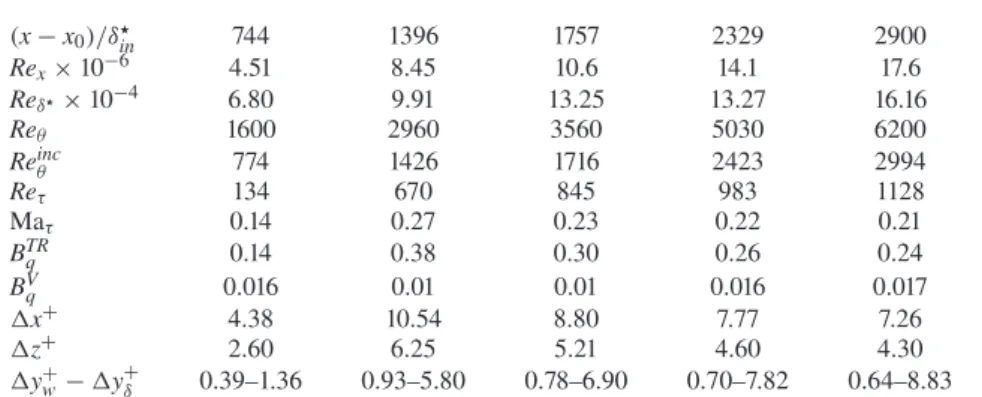
one located in the laminar region (for purpose of comparison), one in the transitional region and the last three in the turbulent portion of the domain.Table 1reports the values of the Reynolds number based on the distance from the leading edgeRe_x =ρeu_ex/μe at the selected stations and some boundary-layer properties. The Reynolds number based on the local momentum thicknessRe_θ =ρeu_eθ/μe(withθ =_δ

0 ρu/ρeu_e(1−ρu/ρeu_e)dy) reaches values close to ≈6000 in the fully turbulent region, corresponding to Re^inc_θ = Re_θμe/μw of approximately 3000. The displacement-thickness-based Reynolds number Re_δ=ρeu_eδ/μe and the friction Reynolds number Re_τ =ρwu_τδ/μw reach values up to ≈16×10⁴ and ≈1100, respectively. Of note, the grid spacings ensure a DNS-like spatial resolution everywhere. Here, the notation ‘•⁺’ denotes normalization with respect to the viscous length scalel_v =μw/(ρwu_τ). Unless otherwise specified, the wall-normal evolution of statistics is displayed in inner semi-local units y= ¯ρu_τy/μ¯, with u_τ =

√τw/ρ¯.

(x−x0)/δin 744 1396 1757 2329 2900

Rex×10⁻⁶ 4.51 8.45 10.6 14.1 17.6

Re_δ×10⁻⁴ 6.80 9.91 13.25 13.27 16.16

Re_θ 1600 2960 3560 5030 6200

Re^inc_θ 774 1426 1716 2423 2994

Re_τ 134 670 845 983 1128

Ma_τ 0.14 0.27 0.23 0.22 0.21

B^TR_q 0.14 0.38 0.30 0.26 0.24

B^V_q 0.016 0.01 0.01 0.016 0.017

Δx⁺ 4.38 10.54 8.80 7.77 7.26

Δz⁺ 2.60 6.25 5.21 4.60 4.30

Δy⁺_w−Δy⁺_δ 0.39–1.36 0.93–5.80 0.78–6.90 0.70–7.82 0.64–8.83

Table 1. Boundary-layer properties at five selected downstream stations. In the table,Ma_τ =u_τ/c_w is the friction Mach number,B^TR_q =q^TR_w/(ρwu_τh_w)andB^V_q =q^V_w/(ρwu_τh_w)are the roto-translational and vibrational dimensionless heat fluxes. Lastly,Δx⁺,Δy⁺w,Δy⁺_δ andΔz⁺denote the grid sizes in inner variables in the x-direction,y-direction at the wall and at the boundary-layer edge and in thez-direction, respectively.

3. Results

3.1. Global flow properties

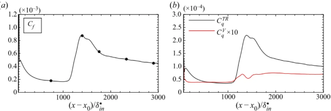
The streamwise evolution of selected quantities at the wall is first discussed.Figures 2(a) and 2(b) report the distributions of the skin friction coefficient C_f and the heat flux coefficientsC_qandC^V_q, defined as

C_f = 2τw

ρeu²_e, C_q^TR= q^TR_w

ρeu³_e, C_q^V = q^V_w

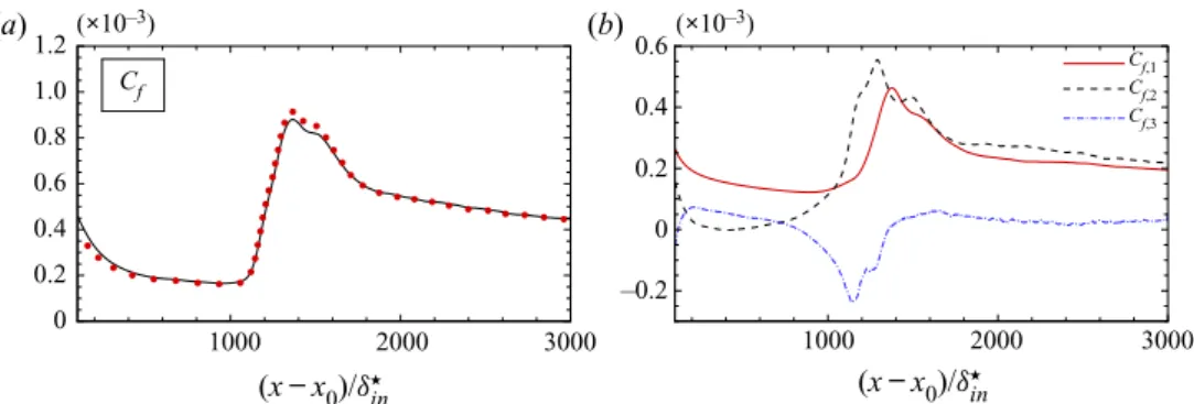
ρeu³_e, (3.1a–c) the net total heat flux being given by the sum of the two contributions. A ramp up starting at(x−x₀)/δ_in ≈1100 leads to a sharp overshoot in the C_f profile, with a peak of the wall shear stress almost five times larger than its corresponding laminar value. The flow achieves a turbulent regime starting from(x−x₀)/δ_in ≈1800, with a smoothly decreasing C_f up to the end of the computational domain. The roto-translational contribution of the wall heat flux C_q^TR is shown to be largely predominant with respect to the vibrational counterpartC_q^V(which is multiplied by ten to match the range offigure 2b), mainly because of the vibrational thermal conductivity λV, whose values are approximately one order of magnitude smaller than λTR. While C^TR_q closely follows the skin friction coefficient profile,C_q^V exhibits a different evolution. It rapidly decreases after the forcing strip and stays approximately constant up to the breakdown to turbulence; afterwards, the value in the turbulent region almost doubles the one in the laminar regime and keeps a constant value up to the end of the domain. The different trend of the heat fluxes is related to the evolution of vibrational temperature gradients across the boundary layer, as discussed later in §3.3. In order to isolate the contributions of the mean and fluctuating field to the skin friction, the decomposition of Renard & Deck (2016) (later extended to compressible flows by Liet al.2019) has been computed; of note, the general hypotheses under which it is derived allows a straightforward application even in presence of thermal and chemical non-equilibrium effects. The skin friction coefficient can then be rewritten under the

1000 2000 3000 0

0.2 0.4 0.6 0.8 1.0 1.2

(x−x₀)/δ_in ¹⁰⁰⁰(x−x₀)/δ_in^{2000 3000}

0 0.5 1.0 1.5 2.0 2.5 3.0

C_q^V ×10 C_f

(×10^–3) (×10^–4)

(a) (b)

C_q^TR

Figure 2. Evolution of (a) the skin friction coefficientCf (black line) and (b) the heat flux coefficientsC^TR_q andC^V_q (black and red lines, respectively). The filled symbols in (a) denote the streamwise location of the five stations selected intable 1.

following form:

C_f = 2 ρ_∞u³_∞

_δ

0 τxy∂u˜

∂ydy ! "

C_f,1

+ 2 ρ_∞u³_∞

_δ

0 −ρuv∂u˜

∂ydy ! "

C_f,2

+ 2 ρ∞u³_∞

_δ

0

(˜u−u_∞)

#

¯ ρ u˜∂u˜

∂x + ˜v∂u˜

∂y

− ∂

∂x

τxx− ¯ρu$u− ¯p% dy

! "

Cf,3

, (3.2)

where C_f,1, C_f,2 and C_f,3 represent the mean-field molecular dissipation, the turbulent dissipation and the effects related to boundary-layer spatial growth, respectively. The sum of the three terms and their separate contributions are displayed infigure 3. An excellent agreement with respect to the directC_f computation is observed in the pseudo-laminar and fully turbulent regions, with only minor deviations in the transition region. TheC_f,3 contribution is negligible everywhere but at the breakdown-to-turbulence location, where it takes negative values due to the abrupt thickening of the boundary layer. The decrease ofC_f,3is counterbalanced by a large increase of the Reynolds stress-related term, whereas the growth of the mean-field contribution,C_f,1, is slightly delayed with respect to the other two. In the turbulent region,C_f,1 andC_f,2 are almost superposed, differently from what observed by Passiatoreet al.(2021) where the former was shown to be predominant. Such a discrepancy can be ascribed to the much larger friction Reynolds numbers reached in the current configuration, leading to an increased turbulent contribution (Fan, Li & Pirozzoli 2019).

3.2. Mean flow analysis

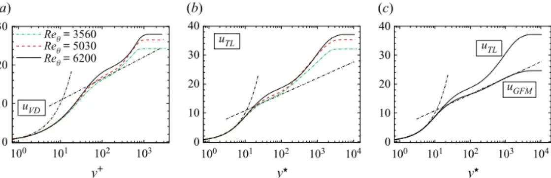
Different scalings for the profiles of the averaged streamwise velocity have been tested.

First, the transformations of Van Driest (1956) and Trettel & Larsson (2016) u_VD= 1

u_{τ u¯}

0

ρ¯ ρw

du, u_TL= _u¯

0

¯ ρ ρw

# 1+1

2 1

¯ ρ

dρ¯ dyy− 1

¯ μ

dμ¯ dyy

%

du (3.3a,b) are shown for the three turbulent stations infigures 4(a) and4(b), respectively. The former scaling has been shown to work reasonably well for adiabatic boundary layers, even at

1000 2000 3000 0

0.2 0.4 0.6 0.8 1.0 C_f

1.2(×10^–3) (×10^–3)

1000 2000 3000

–0.2 0 0.2 0.4 0.6

(x−x₀)/δ_in (x−x₀)/δin

C_f,1 C_f,2 C_f,3

(b) (a)

Figure 3. Evolution of (a) the skin friction coefficientCf(black line) and Renard–Deck decomposition (red symbols) and (b) separate contribution of each term of (3.2).

high speeds (Passiatoreet al.2021). On the other hand, it becomes inaccurate when highly cooled configurations are considered, whether they be boundary layers (Zhanget al.2018;

Huanget al.2020), pipe flows (Ghosh, Foysi & Friedrich2010) or channel flows (Modesti

& Pirozzoli 2016; Sciacovelli, Cinnella & Gloerfelt2017). Figure 4(a) confirms such a trend, both the linear and logarithmic regions being offset with respect to the analytical laws. Of note, in figure 4 the logarithmic region is described by (1/κ)logy⁺+C and (1/κ)logy^∗+C, with κ =0.41 and C=5.2. The semi-local scaling of Trettel &

Larsson, as expected, improves the near-wall prediction since it explicitly accounts for the stress-balance condition within the entire inner layer. A large scatter is, however, observed in the logarithmic region which shows aRe-dependence similar to the van Driest scaling.

Although such a scaling works reasonably well for internal flows, it is not as good for external configurations, most likely because of an interaction with the wake region which is shown to be over-stretched infigure 4(b). Recently, Griffin, Fu & Moin (2021) proposed a new total-stress-based transformation (called hereafter Griffin–Fu–Moin scaling,u_GFM) with a constant-stress-layer assumption, which reads

u_GFM = _δ

0

1 μ⁺

∂u⁺

∂y^∗ 1+ 1

μ⁺

∂u⁺

∂y^∗ −μ⁺∂u⁺

∂y⁺

dy^∗ (3.4)

whereμ⁺denotes normalization of the mean viscosity with respect to its wall value. Such a scaling has been shown to successfully collapse channels, pipe flows and boundary-layer configurations, even at large Mach numbers. A comparison betweenu_TLand u_GFM as a function ofy is shown infigure 4(c) for a velocity profile extracted at Re_θ =6200. In the inner layer, viscous stresses are predominant and roughly correspond to the total shear stress resulting in a very good collapse for both scalings. On the contrary, turbulent shear stresses become dominant in the logarithmic region, which effect is most correctly taken into account by the total-stress-based scaling. This results in a better collapse ofu_GFMonto the universal logarithmic profile with respect tou_TL, for which the slope of the logarithmic region is largely overestimated. Yet, theu_GFM transformation still predicts a higher slope and intercept in the logarithmic region compared with the classical incompressible values, in accordance with the recent study of Lee, Martin & Williams (2021). Finally, we verified that the transformation based on the constant-stress-layer assumption (i.e.τ/τw≈1 across the boundary layer, leading to (3.4)) and the one based on the actual total shear stress (extracted from DNS data) do not exhibit any discernible differences, confirming the

10⁰ 10¹ 10² 10³ 10⁰ 10¹ 10² 10³ 10⁴ 0

10 20

30 Re_θ = 3560 Re_θ = 5030 Re_θ = 6200

y⁺ y

10⁰ 10¹ 10² 10³ 10⁴ y

u_VD

u_TL

u_TL

u_GFM

0 10 20 30 40

0 10 20 30 40 (b)

(a) (c)

Figure 4. Wall-normal profiles of (a) the van Driest-transformed streamwise velocity, (b) Trettel & Larsson’s transformation and (c) comparison between Trettel & Larsson transformation and total-stress-based scaling of Griffinet al.(2021) atRe_θ =6200.

validity of the constant-stress-layer hypothesis. Neither chemical activity nor thermal relaxation process should substantially alter the validity of the transformation since a certain degree of decoupling is observed between the thermochemical and turbulent activities, as previously noticed by Passiatoreet al.(2021) and Di Renzo & Urzay (2021).

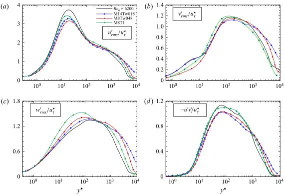
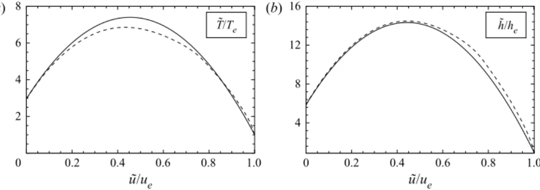
Figure 5 shows the Reynolds stress profiles at the turbulent station Re_θ =6200 normalized with respect to the semi-local friction velocity u_τ; results are compared with low-enthalpy configurations extracted from Zhang et al. (2018) (cases M14Tw018 and M8Tw048) and Xu et al. (2021) (case M8T1). Despite the important differences in the values of the free-stream Mach numbers, friction Reynolds numbers, absolute wall temperatures and wall-cooling rates, the turbulent intensity profiles are comparable and do not exhibit any marked influence attributable to TCNE effects. Consistently with previous observations (Duanet al.2011; Laghaet al.2011; Zhanget al.2018), the larger streamwise component and the smaller cross-flow one may indicate the presence of strong compressibility effects, as discussed later in §3.6. Another scaling often investigated in wall-bounded compressible turbulence is the one that relates the mean velocity to the mean temperature profile for zero-pressure-gradient boundary layers. The modified Crocco relation derived by Walz (1969) writes

T˜ T_e = T_w

T_e +T_aw−T_w T_e

˜ u u_e

+T_e−T_aw T_e

˜ u u_e

2

, (3.5)

withT_aw/T_e =1+r((γ −1)/2)M_e²andrthe recovery factor set equal to 0.9; the relation is shown in figure 6(a). In previous studies with high Mach numbers, wall-cooled, high-enthalpy boundary layers (Duan & Martín2011b), it was found that such a relation deviates from the exactT˜/T_e profile extracted from DNS data; a significant discrepancy is indeed shown in the range 0.2<u˜/u_e<0.7. This should not be surprising since relation (3.5) was derived under calorically perfect gas hypotheses. In order to remove the explicit dependence on thermal and chemical models, Duan & Martín (2011b) proposed an analogous enthalpy-based equation, which reads

˜ h h_e = h_w

h_e +h_aw−h_w h_e f u˜

u_e

−r u²_e 2he

˜ u u_e

2

, (3.6)

where h_aw=h_e+¹₂ru²_e. The function f(u˜/u_e) has to be independent of free-stream conditions, wall temperature and surface catalysis (if any). For calorically perfect gases,