Estimation of the composition of cosmic rays using the radio signal

(1)

HAL Id: tel-01427261

https://tel.archives-ouvertes.fr/tel-01427261

Submitted on 5 Jan 2017

HAL is a multi-disciplinary open access archive for the deposit and dissemination of sci-entific research documents, whether they are pub-lished or not. The documents may come from teaching and research institutions in France or abroad, or from public or private research centers.

L’archive ouverte pluridisciplinaire HAL, est destinée au dépôt et à la diffusion de documents scientifiques de niveau recherche, publiés ou non, émanant des établissements d’enseignement et de recherche français ou étrangers, des laboratoires publics ou privés.

radio signal

Florian Sylvain Gate

To cite this version:

Florian Sylvain Gate. Estimation of the composition of cosmic rays using the radio signal. High Energy Physics - Theory [hep-th]. Ecole des Mines de Nantes, 2016. English. �NNT : 2016EMNA0295�. �tel-01427261�

(2)

Florian GATÉ

Mémoire présenté en vue de l’obtention du

grade de Docteur de l'Ecole des Mines de Nantes

sous le sceau de l’Université Bretagne Loire

École doctorale : 3MPL

Discipline : Constituants élémentaires et physique théorique Spécialité : Cosmologie et astroparticules

Unité de recherche : Laboratoire Subatech UMR6457

Soutenue le 26/10/2016

Thèse N° : 2016EMNA0295

Estimation of the composition of cosmic rays

using the radio signal

JURY

Rapporteurs : M. Jacob LAMBLIN, MCF Université Grenoble Alpes, Laboratoire de Physique Subatomique et de Cosmologie de Grenoble. M. Gilles MAURIN, MCF Université Savoie Mont-Blanc, Laboratoire d’Annecy-le-Vieux de Physique des Particules.

Examinateurs : M. Pol-Bernard GOSSIAUX, Professeur Ecole des Mines de Nantes, Laboratoire Subatech de Nantes.

Mme Marianne LEMOINE-GOUMARD, Chargée de Recherche CNRS, Centre Etudes Nucléaires de Bordeaux Gradignan. Mme Isabelle LHENRY-YVON, Directrice de Recherche CNRS, Institut de Physique Nucléaire d’Orsay.

M. Vincent MARIN, Docteur en Physique, Incubateur de l’Ecole des Mines de Nantes. M. Ginès MARTINEZ, Directeur de Recherche CNRS, Laboratoire Subatech de Nantes. Directeur de Thèse : M. Benoît REVENU, Directeur de Recherche CNRS, Laboratoire Subatech de Nantes.

(3)

(4)

Acknowledgments

Je remercie Bernd Grambow, directeur du laboratoire Subatech, de m’avoir permis de réaliser cette thèse au sein de ce laboratoire. Je tiens également à remercier l’ensemble des personnes qui ont acceptés de faire partie de mon jury de thèse. Merci à Isabelle Lhenry-Yvon d’avoir présidé ce jury, merci à Marianne Lemoine-Goumard, Pol-Bernard Gossiaux et Ginès Martinez. Enfin, je remercie Gilles Maurin et Jacob Lamblin d’avoir chacun endossé le rôle de rapporteur.

J’ai découvert le groupe Astro de Subatech lors de mon stage de M2. Le courant est très vite passé avec l’ensemble de l’équipe et je tiens à remercier chacun d’entre eux pour leur disponibilité, leur franchise mais aussi pour leur amitié.

Je tiens à remercier tout particulièrement mon directeur de thèse Benoît Revenu. Travailler et apprendre à tes cotés au cours de ces trois années fut un réel plaisir. Merci pour tes conseils, ta patience et ton enthousiasme. Nos échanges quasi quotidiens m’ont apporté énormément. Je te remercie également pour la grande confiance que tu m’as accordée et pour la liberté dont j’ai pu profiter pour réaliser ces travaux.

Je veux remercier Vincent Marin qui m’a encadré depuis mon stage de M2 jusqu’à la première moitié de ma thèse. Merci pour cet enthousiasme qui te caractérise et qui est très communicatif. J’ai appris énormément à tes cotés. Nos échanges ont continué bien au-delà du cadre de la thèse même après ton départ du groupe. Les rendez-vous café du matin sont vite devenus indispensable, surtout en fin de thèse. Je te souhaite toute la réussite dans ta nouvelle aventure, tu le mérites.

Je remercie Richard Dallier, toujours disponible pour prêter une oreille attentive et formidable compagnon de voyage. Je garderai toujours un souvenir ému de nos assados en Argentine et de la collocation en péniche aux Pays-Bas.

Enfin je veux remercier Lilian Martin. Merci pour ta franchise et tes conseils lors de nos discussions ainsi que ton aide précieuse pour l’analyse des données CODALEMA. Merci au groupe Astro, ça sera très compliqué de vous rendre tout ce que vous m’avez donné durant ces trois années.

Merci à Jean-Luc Beney, Didier Charrier et Fréderic Lefèvre pour leur enthousi-asme. Merci Fréderic de m’avoir donné l’opportunité de participer au Café des Sci-ences, ce fut une super expérience.

Un grand Merci à Pol-Bernard Gossiaux d’avoir accepté de faire partie de mon jury de thèse et de m’avoir permis d’enseigner à l’Ecole des Mines de Nantes, qui a été une expérience très enrichissante.

Je voudrais également remercier Thierry Gousset, que j’ai eu la chance d’avoir comme enseignant de la première année de licence jusqu’à la dernière année de master.

(5)

Ses conseils m’ont été d’une grande aide lors de mes choix au cours du M2. Merci à Julien Masbou pour son aide et ses précieux conseils pour ma recherche de post doc. Merci à Rémi Maurice pour son aide sur la polarisabilité des molécules

I would like to address special thanks to the Auger Collaboration, in particular to Tim Huege, Julian Rautenberg, Sebastian Mathys, Qader Dorosti and Christian Glaser for the numerous discussions and advice related to AERA. Thanks for everything! I hope to see you during the next ICRCs.

Je remercie l’ensemble des personnes des services administratif et informatique de Subatech qui ont contribué à résoudre de nombreux problèmes et à me faciliter grande-ment la vie. Merci égalegrande-ment à Delphine Turlier et Michelle Dauvé pour leur aide et leur disponibilité.

Je voudrais remercier les personnes avec lesquelles j’ai partagé le bureau H125, les nouveaux comme les anciens. Merci à Jennifer, Guillaume, Zak, Fanny, Grégoire, Loïc, Antony. Je remercie également l’ensemble des thésards et post docs de Subatech pour leur bonne humeur et pour tous les bons moments partagés. Merci à Alexandre S., Thiago, Thorben, Loïck, Kévin, Daniel, Benjamin, Audrey, Gabriel, Florian et Flavia. Enfin merci à ceux qui avec le temps sont devenu mes amis et qui ont donné une saveur particulière à ces trois années. Merci à vous, Javier, Lucia, Lucile, Guillaume, José, Martin, Alexandre P., Christophe et Roland.

Merci à l’équipe de tennis ASPIR, Alexandre, Benoît, Vincent, Christophe, Mas-soud et Catherine avec qui nous avons disputé des rencontres d’anthologie.

Merci à Nicolas Thiolière, Fréderic Yermia et Baptiste ’la gagne’ Léniau d’avoir égayé avec autant de talent, la vie du bâtiment H. Merci à Arnaud Guertin pour ton ami-tié et ta bonne humeur. Je garderai un souvenir impérissable de cette soirée à Chicago.

Je tiens à remercier mes amis pour leur soutien et pour les très nécessaires phases de décompression. Merci, Pierre-Emmanuel, Brieuc, Edwige, Ségolène, Amaury, Thierry, Jean-Sébastien, Gauthier, Maxime, Zak, Nicolas.

Un grand merci à ma famille qui, depuis toujours, m’a apporté son soutien incondi-tionnel. Rien de tout cela n’aurait été possible sans vous. Je remercie aussi ma belle-famille, également venue en nombre le jour de la soutenance. Cela m’a fait très chaud au cœur.

(6)

List of Figures

1.1 Sketch of a torsion balance [1]. . . 9

1.2 Sketch of Wulf’s original electrometer [2]. . . 11

1.3 Dominco Pacini making a measurement of the air ionization [3]. . . 11

1.4 left: Victor Hess after the landing in 1912 [4]. - right: Werner

Kol-hörster during the flight of 1913 [5]. . . 12

1.5 left: Hess measurements up to 5300 m compared to Kolhörster’s results [6, 7]. - right: Kolhörster’s measurements up to 9200 m [7, 8]. - Both

plots are adapted from original papers [9]. . . 13

1.6 Latitude effect curves for the four seasons highlighted by Compton [10]. 14

1.7 Latitude effect caused by the geomagnetic field. The particle arriving towards the poles are represented by the green arrows, those arriving towards the equator, by the red arrows and the red line represents the

equator. . . 15

1.8 Picture of the track left by a positron in Anderson’s cloud chamber,

taken from [11] . . . 15

1.9 View of the north magnetic pole Earth. . . 16

1.10 The Observatoire du Pic du Midi (1937) taken from [12]. . . 17

1.11 Kinematics of a particle entering an interstellar magnetic cloud. A

par-ticle enters a magnetic cloud with a velocity vin and with a pitch angle

θin with respect to velocity of the cloud ~V . After exiting the cloud, the

particle have a velocity voutand under an angle θout. . . 18

1.12 Stochastic distributions of the pitch angle of a particle in a magnetic

cloud. . . 19

1.13 Galbraith and Jelley’s detector composed of a dustbin painted in black, a recycled 25 cm searchlight mirror and a 5 cm phototube, taken from

[13]. . . 20

1.14 Fig 1) Theoretical time between two collision interactions CMB for as

a function of the energy of the proton (107years for 1020eV proton).

-Fig 2) Expected suppression of the energy spectrum for a 5°K and 3°K photon background including the data point from the highest event of

Vulcano Ranch Experiment [14]. . . 23

1.15 Location of several major cosmic rays experiments. The dates are the

data taking periods. . . 24

1.16 Jablonski’s diagram for the fluorescence process. . . 25

1.17 left: picture of the Fly’s Eye experiment showing the 67 modules. -right: arrangement of the mirror along with the PMTs at the focal

(11)

1.18 left: event display for the detected air shower initiated by a 3.2 × 1020

eV primary. - right: longitudinal profile for this event with Xmax≃ 800

g/cm2_[16]. _{. . . 26}

1.19 Energy spectra for (top) Akeno, (middle) Haverah Park, (bottom) Yakutsk

[17]. . . 27

1.20 Energy spectrum obtained with monocular events with Fly’s Eye [17]. . 28

1.21 Energy spectrum obtained with stereoscopic events with Fly’s Eye [17]. 28

1.22 Final results of the energy spectrum from AGASA [18]. . . 29

1.23 Final results of the energy spectrum from HiRes [19]. . . 30

1.24 The atmospheric depth at which the number of secondary particles is maximum as a function of the energy, compared to the mean proton and iron nucleus behavior predicted by three high energy hadronic

in-teraction models [19]. . . 30

1.25 Schematic view of an extensive air shower initiated by a hadron [20]

(see text for details). . . 31

1.26 Left: Number of particles composing a shower initiated by a 3 × 1020

eV vertical proton as a function of the atmospheric depth, sampled by

13 g/cm2steps. - Right: Energy fraction of each type of particle [21]. . 33

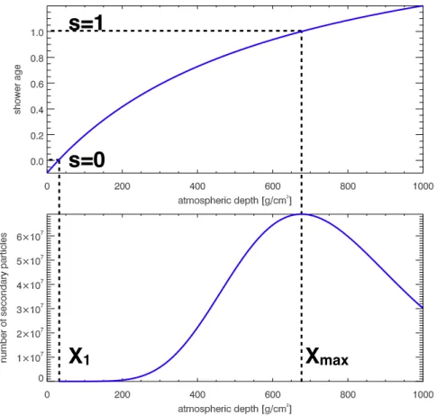
1.27 The geometry of an EAS with the key parameters X1, Xmax, Xinf. . . 33

1.28 Top: the shower age (s) as a function of the atmospheric depth - Bottom: number of secondary electrons and positrons calculated with the GIL

parametrization as a function of the atmospheric depth. . . 35

1.29 p-air and Fe-air probability of the first interaction depth for an energy

of 1017 _eV._{. . . 36}

1.30 Xmax as a function of X1 according to the GIL parametrization of the

longitudinal profile. . . 37

1.31 X1 distributions of 1076 protons and 1076 iron nuclei induced shower

at 1018_{eV, simulated with QGSJET-II.04.} _{. . . 38}

1.32 (Xmax− X1) distributions for the same set of events than in Figure 1.31. . 38

1.33 Xmaxdistributions of the same set of events. . . 40

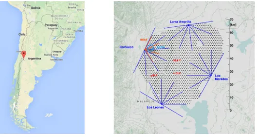
1.34 left: Location of the Pierre Auger Observatory. - right The detection

array. . . 41

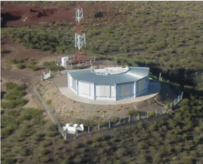
1.35 Aerial view of one of the four fluorescence sites.. . . 42

1.36 Schematic view of a fluorescence telescope of the Pierre Auger

Obser-vatory [22]. . . 42

1.37 Left: Picture of a camera completely assembled with all PMTs and light

collectors in place - Right: Picture of a PMT unit [22]. . . 43

1.38 Event in the field of view of HEAT (telescopes 1 and 2) and Coihueco

(telescope 5) [23]. . . 43

1.39 Schematic view of the conversion of the received light into the energy deposited as a function of the atmospheric depth, taken from [24]. The

(12)

List of Figures xi

1.40 Left: An example of the measured light at the telescope - Right: The energy deposit profile reconstructed from the measured light shown in on the left panel. The line shows a Gaisser–Hillas fit of the profile. The reconstruction of the energy of the primary that induced this shower

gives 3 × 1019eV [22]. . . 45

1.41 Schematic view of a Cerenkov tank, adapted from [25]. . . 45

1.42 An example of a SD event detected by the surface detector array. On the left: particle footprint on the array, the color scale accounts for the signal strength relative to each trigged tank. On the top right: the signal strength as a function of the axis distance, the blue curve is the adjusted NKG function. On the bottom right: zoom on the particle footprint, the color scale accounts for signal strength, thus the particle density at the

ground level. . . 47

1.43 Cosmic ray spectrum, compilation of experimental results. . . 48

1.44 Sketch of the shock acceleration mechanism, taken from [26] (see text

for details). . . 50

1.45 The Hillas diagram [27] (see text for details). . . 51

1.46 Results of the Telescope Array Project on the energy spectrum [28]. . . 52

1.47 Results of the Pierre Auger Observatory on the energy spectrum [29]. . 53

1.48 Sky map in equatorial coordinates highlighting the excess and the deficit of cosmic rays according to their arrival directions at the Telescope Ar-ray experiment, compared to isotropic expectations. The size of the

angular window is 20◦_[28]._{. . . 54}

1.49 Sky map in galactic coordinates highlighting the excess and the deficit of cosmic rays according to their arrival directions at the Pierre Auger Observatory, compared to isotropic expectations. The size of the

angu-lar window is 20◦_[29]. _{. . . 55}

1.50 Measured <Xmax> at the Pierre Auger Observatory [29].. . . 56

1.51 RMS(Xmax) at the Pierre Auger Observatory [29]. . . 56

1.52 Mass composition estimation at the highest energies from Telescope

Array [28]. . . 57

2.1 The main features necessary for a radio detection experiment and their logical interactions. In this sketch, the stations are equipped with two antennas. The signals recorded by the antennas with two polarizations

are represented by the red and blue arrows.. . . 62

2.2 The spherical coordinate system used to calculate the vector effective

length of an antenna. The VEL is indicated by the green arrow. . . 63

2.3 Left: setup of the antenna response calibration (see text for details). Right: Comparison of the measured (red dots) and simulated VEL of the LPDA station at 55 MHz. The error bars and the grey band account respectively for the statistic and systematic uncertainties. Both figures

(13)

2.4 Time series of the voltage recorded with the analog-to-digital converter of an AERA antenna. The signal is filtered to contain only the four beacon frequencies. The periodicity of the beacon beat (around 1.1 µs)

is indicated by the two arrows. . . 65

2.5 Sketch of a plane flying above the AERA array. The ADS-B packets signaling the position of the plane is received by a dedicated device and

the radio stations detect the radio pulses. . . 66

2.6 Left: the broadcasted positions of a plane flying above AERA. Right:

the reconstructed positions from the timing of the pulses at the antennas. 66

2.7 The detection array at CODALEMA with the scintillators represented by the red circles, the radio stations displayed as the black and white

squares and the stations of the compact array displayed as the triangles. 67

2.8 The map of AERA, showing the different deployment stages. The tri-angles are the 3D antennas developed at the Aachen University (upward

triangles) and at the KIT (right-facing triangles).. . . 68

2.9 Left: a logarithmic periodic dipole antenna (LPDA) installed at AERA (phase one). Right: butterfly antennas installed during phase two or

three. Both set up have two horizontal polarizations.. . . 69

2.10 Power spectra measured at AERA as a function of the azimuthal direc-tions for the horizontal polarization (left) and for the vertical polariza-tion (right) in the 1 to 120 MHz frequency band (see text for details). The color scale represents the spectral power in dBm/MHz. Plots are

taken from [31]. . . 70

2.11 Power spectra measured at AERA as a function of the local sidereal time for the north-south polarization (top) and east-west polarization (bottom) in the 1 to 100 MHz frequency band (see text for details).

Plots are taken from [31]. . . 71

2.12 Time series of the electric field induced by a shower event and recorded by an AERA antenna in the east-west polarization (black) and

north-south polarization (red), filtered in the band 30 - 80 MHz. . . 71

2.13 Time series of the electric field in the three polarizations. The total electric field is represented by the dashed line and is calculated as the square root of the quadratic sum of Hilbert envelops (see text for

de-tails). Taken from [32, 33]. . . 72

2.14 Correlation between the energy of the primary and the strength of the electric field as measured by the LOPES experiment [34] by energy bin

(left) and by the CODALEMA experiment (right) [35] . . . 73

2.15 A fit example of the energy fluence with the two dimensional model. The curves are the model values, fitted on experimental data displayed as points, for different directions around the shower axis as a function

(14)

List of Figures xiii

2.16 Deposited energy per unit area for radio stations together with the val-ues given by the model after the fit procedure, the color scale accounts

for the deposited energy [33]. . . 74

2.17 Left: Correlation between the calculated deposited energy from the ra-dio signal and the energy estimated by the particle detectors. The white points are events with 3 or 4 stations with signal and the green ones account for events involving 5 or more stations. The black line is the correlation curve [33]. Right: Scatter around the correlation curve of the left panel for events with five or more antennas [32]. See text for

details. . . 75

2.18 Left: Example of a LDF detected with LOPES, described by a one dimensional exponential decrease. - Right: Correlation of the lateral slope of the electric field and the muon pseudo rapidity measured at the

LOPES and KASCADE experiments. Both figures are taken from [36]. 76

2.19 Difference of the LDF depending on the mass of the primary. Two LDF are simulated with SELFAS, on the left induced by an iron nu-cleus, on the right induced by a proton. The vertical axis represents the atmospheric depth and the horizontal lines accounts for the relative

Xmax depth distributions for proton induced showers and iron nucleus

induced showers. . . 77

2.20 Schematic explanation of the geomagnetic effect. . . 78

2.21 Left: sky map of events detected at CODALEMA, the geographic north is located to an azimuth angle of 0° (top) and the east to an angle of 270° (right). The direction of the geomagnetic field is indicated by the red point. Right: the corresponding 10° gaussian smoothed sky map.

Both plots are taken from [37]. . . 79

2.22 Schematic explanation of the charge excess effect. . . 80

2.23 The experimentally observed core shift from CODALEMA data. The data set is composed of 216 events. The black dots are the radio core

positions with respect to the particle core positions [38]. . . 81

2.24 Constructive and destructive interferences of the two emission mecha-nisms and the resulting amplitude asymmetry around the shower axis

and core shift of the total electric field [38]. . . 82

2.25 Schematic view of the different quantities used in the calculation of the

polarization (see text for details). The figure is adapted from [39]. . . . 83

2.26 Distribution of the measurements of the parameters a at AERA24. The blue line represents the one σ confidence level of the most probable

value. The figure is taken from [39]. . . 84

2.27 Measured polarization angle at AERA as a function of the predicted ones for a pure geomagnetic emission (left) and a contribution of 14%

(15)

2.28 Electric field induced by a 1018 eV proton arriving from the east with a zenith angle of 30°. It is computed with SELFAS in the conditions of the CODALEMA experiment. The maximum electric field at each antenna is calculated as the maximum of the Hilbert envelop using the 3 polarizations and filtered in the band [1 100] MHz (left) and [100 -200] MHz (right). In both cases, the intersection of the shower axis on

the ground plane is located at the origin of the frame. . . 85

2.29 Power spectrum of the electric field simulated in the same conditions as

for Figure 2.28 for different distances to the shower axis. . . 86

2.30 A total particle track of 15 g/cm2 and the sub tracks of 0.3 g/cm2 as

defined in SELFAS. . . 90

3.1 Absolute radiation diagrams for different values of γ. X and Y are re-spectively the direction of propagation of the particle and the direction

transverse to the direction of propagation. . . 95

3.2 Normalized radiation diagrams for different values of γ.. . . 95

3.3 Normalized distribution of the electric field simulated with SELFAS compared to the model given by Equation (3.3) and fitted on SELFAS simulation. Each black cross represents a simulated antenna. The dis-persion at fixed axis distance are due to the asymmetry of the amplitude

of the electric field around the shower axis. . . 96

3.4 Normalized distribution of the electric field simulated with SELFAS and filtered in the frequency band [30 - 80] MHz, compared to the

model given by Equation (3.3). . . 97

3.5 The root mean square angle of the emission of radiation as a function

of γ for the model proposed in Equation (3.5) (see text for details). . . . 98

3.6 Geometry of the problem (see text for details). . . 98

3.7 Amplitude of the electric field of a simulated event as a function of the

angle of emission and the distance to the shower axis. . . 99

3.8 De values reconstructed for identical events but with different zenith

angles . . . 99

3.9 Reconstructed depth of the emission maximum, compared to the depth

of the first inflection point of the shower profiles (Xinf) used to simulate

the electric field with SELFAS. The simulated primaries have an energy

of 1018 eV.. . . 101

3.10 Density map of the maximum electric field received by several

anten-nas, projected into the plane perpendicular to shower arrival direction. . 102

3.11 The one dimensional model (green curve) is fitted on the simulated data points (black points) along the North - South direction. The two

dimen-sional fit is represented by the red curve. . . 103

(16)

List of Figures xv

3.13 Reconstructed Xinfvalues using the 2D model as a function of the

sim-ulated ones for different first interaction depths (X1). The blue line

rep-resents a one to one correlation. . . 104

3.14 Histogram of the differences of the simulated Xinfand the reconstructed

ones for different values of the first interaction depths (X1). . . 104

3.15 Reconstructed Xinf depths for showers induced by protons of 1017 eV,

for different zenith and azimuth angles. The East direction corresponds

to an azimuthal angle of 0° and the South to an angle of 270°.. . . 105

3.16 Left: Core position of the simulated events on the AERA frame, the black crosses refer to the antennas. - Right: Arrival direction of the sim-ulated events, the difference of zenith angle between two grey dashed

lines is of 10°. . . 106

3.17 Simulated Xinf values as a function of the energy of the primary. The

red points are the values of the proton-induced showers and the blue

points are the values of the iron nuclei-induced showers. . . 106

3.18 Left: Reconstructed Xinf values with the two dimensional model as a

function of the expected ones. Right: Histogram of the differences

be-tween the reconstructed values and the reconstructed ones. . . 107

3.19 Reconstructed Xinf values as a function of the energy of the primary.

The red points are the values of the proton-induced showers and the

blue points are the values of the iron nuclei-induced showers. . . 108

3.20 The reconstructed Xinfdistributions with errors propagation. . . 109

3.21 Reconstructed RMS(Xinf) distribution with errors propagation. . . 109

3.22 Simulated LDF with SELFAS for an azimuthal angle of 270° (South) and zenith angles from 5° to 75° with step of 10°. The red curves are the calculated LDF considering an air refractive index of η = 1 (no Cerenkov) and the blue ones with an index of η = 1.00029 (with

Cerenkov), corresponding to the mean value at sea level. . . 112

3.23 The electric field distribution in the east-west direction, induced by a

proton of 1018 eV with a first interaction depth of 5 g/cm2and a zenith

angle of 80° and an azimuth angle of 0° (North) in the frequency band

[30 - 80] MHz. . . 114

3.24 Diagram summarizing the steps of the radio method. . . 115

3.25 Sketch of the case where the low values of the simulated LDF (in blue)

are compared to the detected ones (in red). . . 118

3.26 Comparison of the electric field distributions at 2 tested core positions

and their associated χ2_{test values.} _{. . . 119}

3.27 χ2 density map calculated from the comparison of the experimental

LDF and the experimental data.. . . 120

3.28 Probability distribution of the reconstructed core position in blue

com-pared to the error bars from SD. . . 120

3.29 Probability distribution of the reconstructed energy in blue compared to

(17)

3.30 Agreement between data and simulation as a function of the Xmaxvalues

of the simulated events. . . 122

3.31 Probability distribution of the reconstructed Xmax depth value in blue

compared to the error bars from FD (black vertical lines). . . 122

3.32 Ground position of the fictive array used for the simulations and the

antennas used for the under sampling of the mock event in red. . . 123

3.33 Left: distribution of the differences between reconstructed core position and the simulated one along the East direction - Right: distribution of the differences between reconstructed core position and the simulated

one along the North direction. . . 124

3.34 Left: distribution of the relative differences between reconstructed and true energy. - Right: distribution of the differences of reconstructed and

true Xmax. . . 124

3.35 Left: The contours of the density map are represented by the black

lines. The color scale indicates the values of Log₁₀(χ2). Right: Zoom

on the area of the smallest contour of the density map. The coordinates

defining the contour are represented by the red and green circles. . . 125

3.36 Path finding procedure between two of points defining the contour. . . . 125

3.37 Local contour between two points defining the full contour obtained

with the pathfinding method. . . 126

3.38 The array of simulated antenna used for the comparison in the shower

frame. . . 127

3.39 Correlation plots between the reconstructed easting and northing core positions with the radio method and the SD data. The straight lines

account for a one-to-one correlation. . . 128

3.40 distributions of the differences between the SD core positions and RD

core positions. . . 128

3.41 Left: correlation plot between the reconstructed energy of the primary cosmic ray with the radio method and the SD data. The straight lines account for a one-to-one correlation. Right: distribution of the

differ-ences between the SD energy and RD energy. . . 129

3.42 Correlation plot between the reconstructed Xmax with the radio method

and the FD measurements. The middle straight line accounts for a

one-to-one correlation and the other two account for differences of ± 50g/cm2.130

3.43 Distribution of the differences between the reconstructed Xmaxthe radio

method and the FD measurements. . . 130

4.1 The former flat atmosphere geometry used by SELFAS. . . 135

(18)

List of Figures xvii

4.3 Differences of atmospheric depth calculation between the flat approxi-mation (using equation 4.2) and the spherical description (using equa-tion 4.4) for several zenith angles. The observer is located a the sea level and the shower impacts the ground at the position of the observer. The distance to the observer corresponds to the distance ℓ of the Figures 4.1

and 4.2. . . 137

4.4 Simulated power spectra with the flat approximation (blue curves) and the curved description (red curves) for different distances to the shower axis (50 m, 105 m and 160 m) in the vvv × B direction in the east-west polarization. The showers are induced by protons with a first interaction

depth of 10 g/cm2(left panels) and 100 g/cm2(right panels). . . 138

4.5 Top: Electric field amplitudes simulated with the flat approximation (blue curve) and the curved description (red curve) in the vvv ×BBB direc-tion in the shower frame. The showers are induced by protons with a

first interaction depth of 10 g/cm2and the electric field is filtered in the

band [30 - 80] MHz (left) and [120 - 200] MHz (right) using the three polarizations (maximum of the square root of the quadratic sum of the Hilbert envelop of each polarization). - Bottom: the corresponding rel-ative differences of the amplitude of the electric field at a maximum distance of 200 m from the shower axis, where the emission of the elec-tric field is coherent. The dotted lines account for a relative difference

of ± 10%. . . 139

4.6 Same as Figure 4.5 but for a first interaction depth of 100 g/cm2. . . 140

4.7 Daily variations of the relative humidity as a function of the altitude. . . 141

4.8 Daily variations of the temperature as a function of the altitude.. . . 141

4.9 Daily variations of the total pressure as a function of the altitude. . . 142

4.10 US Standard temperature profile compared to the GDAS profiles at Malargüe. The values are calculated from all the GDAS profiles along the year 2014. For each altitude, the mean, minimum and maximum

temperatures during this year have been computed. . . 144

4.11 Extrema of the differences between the US model air density profile

and all the GDAS profiles along the year 2014. . . 145

4.12 Sketch representing the air density integration along the shower axis up to a geometrical distance ℓ to an observer located at the position O for

different zenith angle θ . . . 146

4.13 Extrema of the atmospheric depth differences between the US Standard model and all GDAS profiles along the year 2014 as a function of source

to observer distance ℓ and for various zenith angles. . . 146

4.14 Gladstone-Dale constant; for Air at T = 288 K . . . 148

4.15 Air refractivity up to 100 km of height, calculated and interpolated from GDAS data in blue, considering a purely dry atmosphere in green and

(19)

4.16 Left: mean deviations along the year 2014 of the air refractivity from

the Gladstone law with ρUS. Right: extremums of the deviations for the

year 2014. . . 149

4.17 Comparison of the Cerenkov ring radius at the sea level for different simulation codes using the GDAS data for the year 2014 at 6 km of height on the left and 16 km of height on the right. In both plots, the

dashed lines account for the extrema obtained for year 2014 with SELFAS.151

4.18 Time series of the electric field simulated with Gladstone(ρGDAS) (blue

curves) and with the high frequency law for the air index with (P,T,PV)GDAS

(red dashed curves) for different distance to the shower axis (6 m, 35 m, 85 m and 160 m) in the vvv × B direction in the east-west polarization.

The first interaction is fixed at 10 g/cm2_. _{. . . 152}

4.19 Same as Figure 4.18 but for a first interaction depth of 100 g/cm2_. _{. . . 153}

4.20 Simulated power spectra with US std. atmosphere with Gladstone(ρUS)

(blue curves) and the a GDAS atmosphere and the high frequency law

for the air index with (P,T,PV)GDAS(red curves) for different distances

to the shower axis (50 m, 105 m and 160 m) in the vvv ×B direction in the east-west polarization. The showers are induced by protons with a first

interaction depth of 10 g/cm2(left panel) and 100 g/cm2(right panel). . 154

4.21 Top: LDFs simulated with US std. atmosphere with Gladstone(ρUS)

(blue curves) and the a GDAS atmosphere and the high frequencies

law for the air index with (P,T,PV)GDAS (red curves), computed with

several antennas in the vvv × B direction. The showers are induced by

protons with a first interaction depth of 10 g/cm2 _{and the electric field}

is filtered in the band [30 - 80] MHz (left) and [120 - 200] using the three polarization. - bottom: the corresponding relative differences at a maximum distance of 200 m from the shower axis, where the emission of the electric field is coherent. The dotted lines account for a relative

difference of ± 10%. . . 155

4.22 Same as Figure 4.21 but for a first interaction depth of 100 g/cm2. . . . 156

4.23 Geometric distance to the observer as a function of the atmospheric

depth using ρUS(black curve) and ρGDAS(dashed red line). See text for

details. . . 158

5.1 Distributions of the measured Xmaxfrom the FD (left) and reconstructed

by the radio method (right) with the same bin size of 70 g/cm2. . . 162

5.2 Top: reconstructed Xmax with the radio method as a function of the

FD measurements, the middle line accounts for a one-to-one

correla-tion and the others account for a deviacorrela-tion of ± 50 g/cm2. Bottom:

distributions of the differences between the radio method and the FD measurements. The plots on the left are obtained with the US Standard

(20)

List of Figures xix

5.3 Xmaxmean values as a function of the energy of the primary by energy

bins. The black dots are the mean Xmax measurements at the Pierre

Auger Observatory obtained with the FD. The green diamonds are the

results obtained with the radio method using the AERA data. . . 163

5.4 RMS(Xmax) mean values as a function of the energy of the primary by

energy bins. The black dots are the RMS(Xmax) measurements at the

Pierre Auger Observatory with the FD. The green diamonds are the

results obtained from the radio method using the AERA data. . . 164

A.1 An example of GDAS data after extracting the values corresponding to

(21)

(22)

List of Tables

1.1 The relative magnitude of the fluxes of the H, He, C, N, O and Z>10

nuclei measured by H. L. Bradt and B. Peters [40]. . . 17

1.2 Results of the gaussian fit of the (Xmax− X1) distributions. . . 39

1.3 Results of the gaussian fit of the Xmax distributions. . . 40

1.4 Energy at which the flux suppression is observed for HiRes, Telescope

Array and the Pierre Auger Observatory. . . 53

3.1 Mean deviations and dispersions of the reconstructed Xinfvalues to the

simulated ones for the 1D and 2D models and for different cuts of the

zenith angle. . . 113

3.2 Reconstructed core position with the radio method (RD) and with the

surface detectors (SD). . . 121

3.3 Energy of the primary cosmic ray reconstructed with the radio method

(RD) and with the surface detectors (SD). . . 121

3.4 Depth of the shower maximum (Xmax) reconstructed with the radio

method (RD) and measured with the fluorescence detectors (FD).. . . . 123

3.5 Mean and standard deviation of the distributions of the differences

be-tween the SD core positions and RD core positions. . . 128

3.6 Mean and standard deviation of the distribution of the differences

be-tween the SD energy and RD energy. . . 129

3.7 Mean and standard deviation of the distribution of the differences

be-tween the FD Xmaxenergy and RD Xmax. . . 131

4.1 Summary of the description of the atmosphere for SELFAS, ZHaireS

and CoRSIKA. . . 134

4.2 Relative differences of the refractivity for GDAS-based models with the US Standard atmosphere and the Gladestone-Dale law for the air index

for several altitudes of interest for air shower physics. . . 150

4.3 Summary of the description of the air refractivity for SELFAS, ZHaireS

and CoRSIKA. . . 151

4.4 Summary of the influence of the description of the atmosphere on the

reconstructed value of Xmax. . . 157

4.5 Improvement of the Xmax reconstruction using the new description of

(23)

(24)

Introduction

The Earth is constantly bombarded by a flux of particles which extraterrestrial ori-gin has been suggested by Domenico Pacini in 1911 and confirmed by Victor Hess in 1912. Many major progress in the fields of particle physics and astrophysics have been achieved thanks to the study of this radiation. The study of cosmic rays is a do-main of the “astroparticles”. Nowadays, the term “cosmic-ray” is used to qualify all charged particles detected on Earth, coming from extraterrestrial sources.

The comic rays energy spectrum extends on more than 32 orders of magnitude for the flux and 12 for the energy. It is described by a power law with a spectral index varying from 2.8 to 2.3. Thus, the number of cosmic-rays decreases very quickly as a function of the energy. The statistics is divided by a factor 100 for each decade in energy. Up to 1017 _{eV, the sources, the acceleration mechanisms and the mass}

compo-sition of the cosmic-rays are well known. In this energy range, the number of events is high enough to allow a direct detection (satellites, balloons . . . ). Above 1017 eV, indirect detection techniques are used and allow the statistical determination of several parameters, as the mass of the primary cosmic rays, with a large number of events.

The indirect detection consists in the observation of the development of the cascade of secondary particles created when a primary cosmic ray interacts with the constituents of the atmosphere. After entering the atmosphere, the cosmic ray interacts after cross-ing an atmospheric depth called X1: it is the first interaction point. The number of

secondary particles increases as long as the energy available in the shower front is suf-ficient, until it reaches the depth of the shower maximum: Xmax, at which the number of

particles is maximum. Beyond this point, the energy is too low to create new particles and their number decreases. Still above 1017eV, the statistics is close to one particle per km2per day, and reaches one particle per km2 per century at 1020 eV. Large detection areas are thus mandatory for the study of ultra-high energy cosmic rays.

It is the case of the Pierre Auger Observatory, in Argentina. This observatory is composed of 1660 Cerenkov tanks covering a surface of 3000 km2, 27 fluorescence telescopes spread across four sites, 153 radio stations and the construction of 61 muon counters has begun. The Cerenkov tanks sample the secondary particles distribution reaching the ground. The muons counters are buried at 2.5 meters under the ground, allows the measurement of the muonic component of the shower, as the electrons and positrons are stopped before reaching this depth. When the air shower crosses the atmo-sphere, the secondary particles that composed it, excite the nitrogen molecules. These molecules go back to their ground energy state by emitting fluorescence light that is received isotropically by the telescopes. The intensity of the light is proportional to the number of particles composing the air shower at the time of the emission. This method

(25)

allows a calorimetric measurement of the air shower development in the atmosphere and especially the direct measurement of the Xmax depth. This latter quantity is highly

correlated to the mass of the primary cosmic ray as it depends, at the first order, on the interaction cross section of the primary with the atmosphere.

At the Pierre Auger Observatory, the mass of the cosmic rays with an energy higher than 1017 eV is statistically determined. The mean measured Xmax by energy range

are compared to the results given by the ultra-high energy hadronic interaction models. This method is effective within the condition that the number of detected air showers is high, which is the case up to 1019 eV. For higher energies, the statistics is very low. A cut-off in the energy spectrum is observed at 6 ×1019eV with a confidence level higher than 20 σ. The GZK limit predicts this cut-off and attributes it to the interaction of the cosmic rays with the photons of the cosmic microwave background for which the energy threshold is estimated to be at 5 ×1019 eV. Moreover, the duty cycle of the fluo-rescence telescopes is around 14% as their sensitivity allow measurements during night without moon and without bad weather. Then, the number of detected events is too low above 4 × 1019_{eV to precisely determine the mass of cosmic rays with this technique.}

Nowadays, there is still some questions about ultra-high energy cosmic rays remain. The cut-off in the energy spectrum is experimentally highlighted but the reason is not clearly defined. The data from the Pierre Auger Observatory, in the Southern hemi-sphere, are compatible with an isotropic flux while the Telescope Array experiment, in the Northern hemisphere, observes an excess of events toward the Ursa Major galaxy cluster. The acceleration and propagation mechanism models at these energies are also poorly constrained due to the lack of data. Finally, at these energies, the main can-didates are the protons and the iron nuclei due to their high abundance and binding energy. The Pierre Auger Observatory data, at the highest energies, are compatible with a progressively heavier composition. The data of the Telescope Array experiment are compatible with protons at all energies. The precise determination of the mass would allow to constrain the acceleration and propagation models and the type of sources. It is then the priority of all experiments devoted to the detection of ultra-high energy cosmic rays. Ideally, measurement of Xmax should be done with a duty cycle, close to 100 %,

as it is the case using radio stations. The atmospheric air showers are mainly made of positrons and electrons (which contribute to 90 % of the total energy, with the photons). The temporal evolution of the net charge of the shower front induces the emission of an electric field in the range detectable in the MHz range of few hundreds of micro Volts per meter for a vertical shower induced by a primary of 1017 _{eV. This detection method}

is sensitive to the full air shower development as for the fluorescence method.

The radio stations of the Pierre Auger Observatory are located on the AERA (Auger Engineering Radio Array) experimental site, close to one of the four sites of fluores-cence telescopes. They allow the detection in coincidence with the telescopes and the Cerenkov tanks. These stations are equipped with two orthogonal antennas of butterfly

(26)

Introduction 3 type or logarithmic dipole antenna type (LPDA). The stations record the electric field in two polarizations (North-South and East-West) in the frequency band [30-80] MHz in order to avoid the radio anthropic emitters (AM frequency band below 20 MHz and FM frequency band above 80 MHz). A detection involving several antennas allow the reconstruction of the lateral distribution function (LDF) of the electric field, calculated as the maximum electric field received by each antennas as a function of their position relatively to the air shower axis.

During my PhD thesis, a reconstruction method of the Xmax depth with the radio

signals has been developed in order to estimate the mass of the cosmic rays at energies above 1017 eV, with a duty cycle close to 100 %. It is now established that the LDF is highly correlated to the Xmax depth. The electric field is highly beamed towards the

direction of propagation of the air shower. A high Xmax value gives a narrow

distribu-tion, as the emission of the electric field occurs close to the ground. On the contrary, a low Xmax value gives a LDF less intense and more spread. The reconstruction method

is based on the comparison of the LDF sampled by the radio stations to an LDF model. In a first step, I have developed a model of angular distribution function of the ra-diation in agreement with experimental observations of the electric field induced by the development of an extensive air shower. A first emission mechanism is due to an ex-cess of negative charges against the positive charges, predicted by Askaryan in 1962. Indeed, the positrons annihilate in the middle. The time variation of the current induced by the net charge of the air shower front produces an electric field radially polarized around the air shower axis. In 1967, Kahn and Lerche predicted another phenomenon. The presence of the terrestrial magnetic field causes a systematic and opposed deviation of the electrons and positrons under the effect of the Lorenz force. It induces a current oriented perpendicularly to the direction of propagation of the air shower. The time variation of this current creates an electric field polarized in the direction vvv × B, with vvv the direction of propagation of the air shower and BBBthe direction of the geomagnetic field. The total electric field emitted by an atmospheric air shower is a superposition of the two mechanisms, which can interfere in a constructive or destructive way depend-ing on the observer relative position around the air shower axis. The developed model takes into account these two mechanisms and has been parametrized with a simulation provided by the code SELFAS. This code uses a microscopic approach by summing up the individual contributions of all secondary particles to the total electric field. It appears that the maximum of emission can be associated to Xinf, the depth at which the

production rate of the secondary particles is maximum. The parametrized model is thus an image of the radiation emitted by an air shower at this depth.

This model has been tested on a set of simulated events. In order to compare several air showers with different zenith angles, the atmospherical effects have been taken into account to convert this distance into atmospheric depth. The used atmosphere model is a parametrization of the US Standard model, giving the crossed atmospheric depth

(27)

corresponding to an altitude.

The comparison of the reconstructed atmospheric depths to the simulated Xinfdepths

are in good agreement. However, this model which predicts an exponential decay of the intensity of the electric field as a function of the distance to the shower axis has some limitations. Indeed, the topology of the electric field at the ground level is more com-plex. An effect similar to the Cerenkov emission occurs. This effect is due to the time compression (secondary particles are relativistic), and is responsible for a boost of the electric field intensity which appears under a particular angle of emission. The value of the angle depends on the velocity of the particles and on the air refractive index.

Thus, another method has been developed, using the SELFAS code as prediction. This method aims to reconstruct all the parameters describing an atmospheric air shower: the air shower core position on the array, the primary energy and Xmax, allowing an

esti-mation of the primary mass. The radio data allow a precise reconstruction of the arrival direction by studying the relative arrival time of the electric field at each antenna posi-tion. The method consists in the simulation of a set of events composed of air showers initiated by iron nuclei and protons with the same arrival direction as the one exper-imentally deduced. The electric field is computed for all antennas of a dense fictive array. After interpolation, the computed LDFs are compared to the experimental data. The first interaction depth of each simulation is randomly drawn in a realistic way with the use of a ultra-high energy hadronic interaction model. Each simulation has a partic-ular Xmax value. The energy of the primaries is arbitrary fixed, as the amplitude of the

computed field varies linearly with the energy of the simulated primary particle. The best agreement is obtained for a particular core position of the air shower, a particular Xmax and amplitude factor. The three reconstructed parameters are compared with the

values obtained from the Cerenkov tanks and the fluorescence telescopes. However, a systematic shift of 17 g/cm2_{is observed.}

In order to explain and correct this deviation, improvements have been applied to SELFAS. The atmosphere geometry was previously computed within a flat Earth ap-proximation where the atmospheric layers were flat. Now, SELFAS uses a realistic and totally spherical description. Secondly, the data produced by the fluorescence tele-scopes take into account the daily and seasonal variations of the atmosphere density. The atmospheric conditions strongly affect the electric field distribution. It is then im-portant to take it into account in order to precisely reconstruct the Xmax depth. The

GDAS (Global Data Assimilation System) provides meteorological data of interest ev-erywhere on Earth every three hours. This database has been used in order to allow a dynamic simulation of the atmosphere, matching as much as possible the experimental conditions at the time of the event detection. Moreover, an estimation of the air refrac-tive index more adapted to the problem is proposed. Indeed, the most widely used law is the Gladstone and Dale law, which proposes a linear variation of the air index as a function of the density. The relative humidity of the air is not taken into account while

(28)

Introduction 5 it has an important influence on the calculation of the air index. In addition, this law is parameterized for optical wave lengths, which is not appropriate to the detection in the decametric range. Therefore, a law that has been specially parameterized for the high and very-high frequencies, taking into account the pressure, the temperature and the relative humidity, has been used. The improved version of SELFAS is finally used for the reconstruction of several events detected at the Pierre Auger Observatory. The estimation of the mass composition of the cosmic rays with energies above 1017 eV is proposed for both experiments.

(29)

(30)

C

HAPTER

1 A history of high energy cosmic rays

1.1 The radiation from above . . . 9 1.1.1 1785 - The very first observation . . . 9 1.1.2 1834 - The mystery of the ionization of the atmosphere . . . 10 1.1.3 1910’s - Time to go up! . . . 12 1.2 First steps towards the nature of cosmic rays . . . 13 1.3 The discovery of the extensive air showers. . . 16 1.3.1 1930’s - Pierre Auger and the discovery of the extensive air showers 16 1.3.2 1949 - Enrico Fermi’s "On the origin of cosmic radiation" . . . . 17 1.3.3 The 1950’s - The birth of gamma astronomy. . . 20 1.3.4 Exploring the highest energies. . . 21 1.4 The era of the ground detectors . . . 22 1.4.1 1960 - The detection of the secondary particles . . . 22 1.4.2 1967 - The ground particle detectors . . . 24 1.5 The fluorescence technique . . . 24 1.6 Physics of the extensive air showers . . . 31 1.6.1 The constituents of the EAS . . . 31 1.6.2 Geometry of the EAS. . . 33 1.6.2.1 The longitudinal profile . . . 33 1.6.2.2 The lateral profile . . . 35 1.6.3 Correlation to the primary cosmic ray . . . 36 1.7 The Pierre Auger Observatory . . . 41 1.7.1 The fluorescence telescopes . . . 41 1.7.2 The Cerenkov tanks . . . 45 1.8 Actual status of cosmic rays. . . 48 1.8.1 Energy spectrum . . . 48 1.8.2 Sources and acceleration mechanisms . . . 49 1.8.3 Flux suppression . . . 52 1.8.4 Anisotropy . . . 53

(31)

1.8.5 Composition . . . 55 1.9 Conclusions. . . 57

After a century of observations, the composition, the sources location and the accel-eration mechanisms of the ultra-high energy cosmic rays are still not clearly established. However, the study of these mysterious particles has led to major discoveries in astro-physics, particle physics and cosmology. In this first chapter, I give a review of the important discoveries that have led to the actual understanding of the cosmic rays at the highest energies, from the first detections to the modern giant experiments.

(32)

1.1. The radiation from above 9

1.1 The radiation from above

1.1.1 1785 - The very first observation

The first observation of the existence of cosmic rays happened back in 1785. At that time Charles Augustin de Coulomb formalized the interaction between two static charges, known nowadays as the Coulomb’s law, written in its scalar form as:

F = keq1_r.q₂1 (1.1)

Where ke= 8.99 × 109 N.m2 C−2 is the Coulomb’s constant, r is the distance

be-tween the charges and q1 and q2are their signed magnitudes. To quantify the

electro-static force, he used a torsion balance (Figure1.1).

Figure 1.1: Sketch of a torsion balance [1].

The device is composed of a bar with a metal coated ball attached to one end, and suspended from its middle by a thin fiber acting as a torsion spring. The electric charge of the ball is known and an other ball of the same polarity was brought near to it. The two balls eventually repelled each other, twisting the torsion spring. The distance

(33)

between the two balls could be read with a scale integrated to the device and knowing the necessary force to twist the spring, Coulomb could estimate the intensity of the force between the two balls. Nevertheless, he also noticed that the device spontaneously discharge, which was eventually due to the flux of cosmic rays in the device but he imputed it to the action of the air and not to the defective insulation of the device, as notified in a report to the France’s Royal Academy of Sciences [1].

1.1.2 1834 - The mystery of the ionization of the atmosphere

In 1834, Michael Faraday introduced the term of ion [41] to describe species that goes from one electrode to another in aqueous medium. One year later, Faraday con-firmed Coulomb’s observation with a better insulation of the device [42]. In 1850, Cano Matteucci followed by William Crookes [43] in 1879, observed that the rate of the dis-charge decreases at lower atmospheric pressure. Faraday’s work allowed Crookes to conclude that the discharge was due to the air conductivity, thus to its ionization. The knowledge of the cause of the discharge kindled the question that will lead to the dis-covery of cosmic rays: what is causing the ionization of the atmosphere? The disdis-covery of the radioactivity by Henry Becquerel in 1896 [44,45] was of great interest to explain the origin of the ionization.

In 1898, Pierre and Marie Curie discovered that polonium and radium undergo trans-mutation through radioactive decay [46], for which they received the Nobel prize in 1903 with Henry Becquerel [47]. They also demonstrated that these radioactive sub-stances can emit charged particles that cause discharge of electroscopes. The level of ionization was then used to gauge the amount of radioactivity [48]. At this point, the search for the main source of natural radioactivity began and the main candidates were the Sun, the soil and the atmosphere. The dominant belief were that the radioactive elements in the ground was the main source of the ionization of the atmosphere.

In the beginning of the 20th century, Wilson [49], Elster and Geitel [50] improved the sensitivity of the technique by putting the electroscope in a closed vessel to ensure a good insulation. In 1901, Wilson’s measurements in tunnels [51] showed no reduction of the ionization rate comparing to the surface and comforted the idea that the main source of radioactivity is in the soil. In 1909, Theodur Wulf perfected the electrometer making it transportable [52]. In 1910, during a holiday trip to Paris in which he brought few of his electroscopes, he measured the ionization of the atmosphere at the bottom and at the top of the Eiffel tower [53].

(34)

1.1. The radiation from above 11

Figure 1.2: Sketch of Wulf’s original electrometer [2].

Wulf’s measurements show that the ionization rate fell from 6 ions by cm3 _{at the}

ground level to 3.5 ions by cm3 at 330 meters above the ground. However if the ion-ization was due to γ rays from the ground, as commonly believed, the ionion-ization rate should have been halved before reaching 100 meters above the ground, following an ex-ponential decrease. These results are incompatible with a source of radiation from the ground and suggested a source from above. In 1911, Domenico Pacini made a serie of measurements, in particular over the sea surface and at 3 meters under water at Livorno and later in Bracciano.

Figure 1.3: Dominco Pacini making a measurement of the air ionization [3].

(35)

the confirmation of a 20% reduction of the ionization rate with a confidence level of 4.3σ [3]. Pacini concluded that "a sizable cause of ionization exists in the atmosphere, originating from penetrating radiation, independent of the direct action of radioactive substances in the soil."[54].

1.1.3 1910’s - Time to go up!

The same year of 1911 Victor Hess, who was working on measuring the absorp-tion coefficients of radioactivity in air, undertook two balloon flights (see Figure 1.4

(left) from Vienna up to 1300 meters to measure the possible variation of the radioac-tivity with the altitude using few Wulf’s electrometers. As no effect was found, seven flights were scheduled from April to August 1912. During the final flight he reached the altitude of 5300 meters [55].

Figure 1.4: left: Victor Hess after the landing in 1912 [4]. - right: Werner Kolhörster during the flight of 1913 [5].

Hess’ results, in Figure 1.5 (left), shows that the ionization rate is decreasing up to 1 km of height as expected. However, it increases as a function of altitude beyond this point. The flight took place during a nearly total sun eclipse. This experimental condition led him to conclude that, not only the ionization was caused by a source of radiation from above, but also that it was not coming from the sun, but further from outer space. The ionization rate reaches ten times the value at sea level. Hess’s results were confirmed by Werner Kolhörster in 1913 (see Figure1.5(left)). Kolhörster made a series of flights between 1913 and 1914 during which he reached an altitude of 9300 meters (see Figure1.4(right)).

(36)

1.2. First steps towards the nature of cosmic rays 13

Figure 1.5: left: Hess measurements up to 5300 m compared to Kolhörster’s results [6,7]. - right: Kolhörster’s measurements up to 9200 m [7,8]. - Both plots are adapted from original papers [9].

The second flight of Kolhörster took place on 28th June 1914 (at 9300 meters), the results, presented in Figure 1.5 (right), are in agreement with his previous measure-ments. The same day the assassination of Archduke Franz Ferdinand of Austria took place, leading to the start of World War I. During this period and the years after, no new measurement series have been achieved and investigations stopped.

1.2 First steps towards the nature of cosmic rays

Around 1925, researches started again, mainly in the USA. The data transmission tech-nology developed during the war was used by Millikan and Bowen to launch unmanned balloons carrying their newly engineered very light electrometer (around 200 g) and ion chamber. Throughout flights in Texas up to 1500 meters, they found a radiation inten-sity of one fourth the inteninten-sity reported by Hess and Kolhörster [56]. At that time they were unaware that a latitude geomagnetic effect exists and they explained this observa-tion as an inversion of the radioactivity intensity at higher altitudes. Millikan concluded that there was no extraterrestrial radiation and stated to the American Physical Society: "The whole of the penetrating radiation is of local origin.", which will be strongly ar-gued by Arthur Compton [57]. It was believed that cosmic rays were composed of γ rays due to their important penetrating power and also because the penetrating power of relativistic charges was unknown. In 1926, Millikan and Cameron reproduced Pacini’s experiment, stating that these particles shoot through space equally in all directions, and called them "cosmic rays" [58]. Millikan was skillful at handling medias and, in the United States, the discovery of cosmic rays quickly became an american success. The geomagnetic effect experienced by Millikan was accidentally discovered in 1927

(37)

by Clay [59] when carrying his detector on a trip from Java to the Netherlands. He ob-served that the ionization rate was minimum at the magnetic equator and higher farther south or north. He confirmed his results with multiple measurements [60, 61]. Comp-ton recognized the variation as a geomagnetic effect, giving evidence that the radiation consisted of charged particles [62,63].

Figure 1.6: Latitude effect curves for the four seasons highlighted by Compton [10].

Measurements at 69 locations from 1931 to 1933 demonstrated the dependence of cosmic radiation intensity on geomagnetic latitude [64]. The record of cosmic rays intensities measured during 12 trips between Vancouver, Canada and Sydney, Australia, led by Compton from March 1936, to January 1937 [10] are shown in Figure1.6. The charged particles approaching the Earth near the poles travel almost along the direction of the magnetic lines of force. They experienced no deviation and easily reach the surface of the Earth and hence maximum intensity at poles. But the charged particles that approach towards the equator have to travel in a perpendicular direction to the field and are deflected away. Only particles with sufficient energy can reach the equator, while the low energy particles are deflected back into cosmos and hence minimum intensity at the equator as depicted in Figure 1.7. This discovery put an end to the Millikan’s theory, which specified that cosmic rays were composed of γ rays.

(38)

1.2. First steps towards the nature of cosmic rays 15

E

W

S

N

Figure 1.7: Latitude effect caused by the geomagnetic field. The particle arriving to-wards the poles are represented by the green arrows, those arriving toto-wards the equator, by the red arrows and the red line represents the equator.

In 1932 and under the supervision of Millikan, Anderson began to investigate on cosmic rays in the frame of the preparation of its PhD thesis. During a course in which he was studying the tracks that cosmic particles produce in a Wilson chamber [65], he stumbled upon unexpected tracks that must have been created by a particle of the same mass as the electron but of opposite electric charge.

Figure 1.8: Picture of the track left by a positron in Anderson’s cloud chamber, taken from [11]

He interpreted correctly the first observation of the positron [11], the antiparticle asso-ciated to the electron and theoretically predicted by P. Dirac in 1932 [66].

(39)

In 1933, Rossi and others demonstrated that the intensity of the cosmic radiation is larger from the east than from the west [67]. The trajectory of cosmic rays is eventu-ally bended by the presence of the Earth magnetic field, as previously highlighted by Compton. As depicted in Figure1.9if more comic rays are detected from the east, it is because most of them are positively charged particles.

from the east, allowed trajectory

~

B

geo

from the west, forbidden trajectory

Figure 1.9: View of the north magnetic pole Earth.

In the 30’s Rossi [68] also noticed simultaneous discharge in two Geiger counters separated by several meters, far in excess to be chance coincidences. At the time he stated: "It would seem that occasionally very extensive groups of particles arrive on the equipment".

1.3 The discovery of the extensive air showers

1.3.1 1930’s - Pierre Auger and the discovery of the extensive air

showers

At the end of the 30’s, Pierre Auger and collaborators observed the same phe-nomenon when they undertook a systematic survey [69], first at the Observatoire du Pic du Midi (2876 m) in France and at the scientific station of Jungfraujoch (3500 m) in Switzerland. Two detectors located many meters apart horizontally (as far as 75 meters) both have detected the arrival of particles at exactly the same time. In the meantime the rate of coincident detections dropped drastically with the distance between the detectors from 10 cm to 10 m and decreased slowly at larger distances but once again the event rates were too high to be due to chance coincidences.

(40)

1.3. The discovery of the extensive air showers 17

Figure 1.10: The Observatoire du Pic du Midi (1937) taken from [12].

The results allowed Pierre Auger’s team to conclude that the detected particles are secondary charged particles produced by the interaction of a very energetic cosmic ray with the atmosphere constituents. They stated that the energy of the primary particles could exceed one million GeV, which is more energetic than the maximum energies that modern particle accelerators can reach, even with the Large Hadron Collider at CERN (Switzerland).

In 1940 and 1941, M. Schlein et al. determined that cosmic rays are mostly protons [70, 71]. In 1948, H. L. Bradt and B. Peters measured the relative flux of cosmic rays for different nuclei [40] and the distribution of atomic numbers among the primaries was determined without any energy cut:

nucleus H He C, N, O Z>10

relative ratio 4000 1000 35 10

Table 1.1: The relative magnitude of the fluxes of the H, He, C, N, O and Z>10 nuclei measured by H. L. Bradt and B. Peters [40].

They found that even if protons and helium nuclei are the main part of cosmic rays, heavy particles are a significant fraction of the total cosmic rays flux.

1.3.2 1949 - Enrico Fermi’s "On the origin of cosmic radiation"

The first description of the energy spectrum was introduced by Enrico Fermi in the article "On the origin of cosmic radiation" in 1949 [72], where he exposed his theories on the acceleration mechanisms. Fermi’s intuition, which led him to assume