RESEARCH OUTPUTS / RÉSULTATS DE RECHERCHE
Author(s) - Auteur(s) :
Publication date - Date de publication :
Permanent link - Permalien :
Rights / License - Licence de droit d’auteur :
Bibliothèque Universitaire Moretus Plantin
Institutional Repository - Research Portal
Dépôt Institutionnel - Portail de la Recherche
researchportal.unamur.be
University of Namur
System Requirements. Channel Model Prediction Vanderpypen, Joël; Schumacher, Laurent
Publication date:
2008
Document Version
Early version, also known as pre-print
Link to publication
Citation for pulished version (HARVARD):
Vanderpypen, J & Schumacher, L 2008, System Requirements. Channel Model Prediction: FP6 IST SURFACE
D2.2 v2.0..
General rights
Copyright and moral rights for the publications made accessible in the public portal are retained by the authors and/or other copyright owners and it is a condition of accessing publications that users recognise and abide by the legal requirements associated with these rights. • Users may download and print one copy of any publication from the public portal for the purpose of private study or research. • You may not further distribute the material or use it for any profit-making activity or commercial gain
• You may freely distribute the URL identifying the publication in the public portal ?
Take down policy
If you believe that this document breaches copyright please contact us providing details, and we will remove access to the work immediately and investigate your claim.
IST-4-027187-STP-SURFACE
Start date of project: 1st January 2006
Duration: 36 months
Project co-funded by the European Commission within the Sixth Framework Programme
D2.2 v2.0
System Requirements. Channel Model Prediction
Contractual date of delivery to the EC: December 2006 Actual date of delivery to the EC: January 2008
Editor (s): L. Schumacher
Author (s): J. Vanderpypen, L. Schumacher Workpackage: 2
Estimated person months: 15
Dissemination level1: PU
Nature: Report Version: 2.0
Total number of pages: 86
1 PU: Public, PP: Restricted to other programme participants (including the Commission Services), RE: Restricted to a group specified by the consortium (including the Commission Services), CO: Confidential, only for members of the consortium (including the Commission Services)
File: SURFACE_D2_2_v2_0.doc, January 2008 Page 2 of 86
EXECUTIVE SUMMARY
The SURFACE (Self Configurable Air Interface) project aims at studying and evaluating the performances of a novel generalised air interface capable of self-reconfiguring in order to satisfy global network QoS (Quality of Service) requirements. It considers Multiple Input Multiple Output (MIMO) technologies as an option.
Wireless MIMO channels are being investigated extensively nowadays. Their potential benefits for wireless communications, their higher throughput and the increase of their QoS is desired, and needed by new services of the third generation of cellular networks (3G) and its evolutions (Beyond 3G, B3G).
To improve wireless transmissions, the state of the channel should be known by the transmitter to adapt its transmission policies. So the receiver has to send feedback on the channel state to the transmitter. But when this feedback reaches the transmitter side, it is likely to be outdated, and therefore useless. However, if we use the current channel state to predict its likely future state, we are able to transmit more efficiently.
In this deliverable, we aim at extending existing SISO or MIMO simplified channel models that are suited for designing channel predictors. The document first presents the WINNER’s SCME channel model, which will be the reference channel for testing predictors. Afterwards it introduces the SURFACE channel model, which is derived from the WINNER’s SCME, with parameters adapted to the requirements of the other workpackages.
Several simplified channel models and predictors are then introduced. Two of them seemed particularly relevant for our research work, namely the original ESPRIT algorithm and a modified version by Andersen et al, as having limited computer power requirements. So we investigated and tested them thoroughly. Actually, these two predictors are only for SISO channels, so we extended them into MIMO models.
After several tests which revealed rather good performances, and low quantization feedback robustness, these two MIMO predictors were merged into a single one, taking best of both. The new predictor requires 5 channel observations for a 2x2 MIMO channel, and 17 if 4x4 MIMO. The feedback can be quantized on 2x 4 bits per complex MIMO coefficient without decreasing prediction accuracy. It means it requires 160 bits, collected during 18.75 ms (37.5 LTE TTI) to set up a 2x2 MIMO predictor, and 2,176 bits collected during 63.75 ms (127.5 LTE TTI) to set up a 4x4 one. As far as noise robustness is concerned, performances are similar at SNR of 20 dB and SNR of 100 dB. Performance decreases when SNR is only 3 dB. We finally investigate to topic of rank prediction of the MIMO channel matrix. For that goal, we use the MIMO predictor to get future MIMO channel matrices, and after their quantization, we compute its rank. It seems a floating point quantization is required to avoid zero matrices after rounding, and only 2x 4 bits per complex MIMO channel coefficient is optimal to get the best results.
Due to a late start, a first restricted version of this deliverable was released in January 2007, only reflecting the work of four person months. This final release reflects the work of fifteen person months.
File: SURFACE_D2_2_v2_0.doc, January 2008 Page 3 of 86
DISCLAIMER
The work associated with this report has been carried out in accordance with the highest technical standards and the SURFACE partners have endeavoured to achieve the degree of accuracy and reliability appropriate to the work in question. However since the partners have no control over the use to which the information contained within the report is to be put by any other party, any other such party shall be deemed to have satisfied itself as to the suitability and reliability of the information in relation to any particular use, purpose or application.
Under no circumstances will any of the partners, their servants, employees or agents accept any liability whatsoever arising out of any error or inaccuracy contained in this report (or any further consolidation, summary, publication or dissemination of the information contained within this report) and/or the connected work and disclaim all liability for any loss, damage, expenses, claims or infringement of third party rights.
File: SURFACE_D2_2_v2_0.doc, January 2007 Page 4 of 86 CONTENT LIST LIST OF FIGURES ... 7 LIST OF SYMBOLS... 9 LIST OF ACRONYMS... 11 1 INTRODUCTION... 12
2 THE WINNER’S CHANNEL SIMULATOR ... 13
3 THE SURFACE CHANNEL MODEL ... 14
3.1 INPUT/OUTPUT PARAMETERS... 14
3.2 REMARKS ABOUT THE MODEL... 15
3.3 PATHLOSS ASSUMPTIONS... 15
3.4 LINK LEVEL PARAMETERS... 17
3.5 SYSTEM LEVEL PARAMETERS... 18
4 MODELISATION AND PREDICTION - STATE OF ART ... 19
4.1 THE ROMANTIK MODEL... 19
4.1.1 The SISO model ...19
4.1.2 The MIMO model...20
4.1.3 Comments...20 4.2 APOLYNOMIAL ESTIMATOR... 21 4.2.1 Proposed scheme ...21 4.2.2 Comments...22 4.2.3 Results of computations...22 4.3 AMISO ESTIMATOR... 23 4.4 THE ANDERSEN ET AL. PREDICTOR... 23
5 THE ESPRIT PREDICTOR ... 25
5.1 CHANNEL MODEL... 25
5.2 BASIC IDEA... 25
5.3 THE ESPRIT TECHNIQUE (MATHEMATICAL BACKGROUND) ... 26
5.4 HOW TO COMPUTE THE CORRELATION MATRIX R? ... 29
5.5 COMPUTING THE AMPLITUDES... 30
5.6 PRODUCING PREDICTIONS... 30
File: SURFACE_D2_2_v2_0.doc, January 2007 Page 5 of 86
6 ANOTHER PREDICTOR BASED ON ESPRIT... 32
6.1 BASIC IDEA... 32
6.2 MATHEMATICAL JUSTIFICATION... 33
6.3 DIFFERENCES BETWEEN THIS ALGORITHM AND ESPRIT ... 34
6.4 SUMMARY ALGORITHM... 34
7 SISO COMPUTATIONS... 35
7.1 SAMPLE COMPUTATIONS... 35
7.2 PERFORMANCE INDICATOR... 38
7.3 PERFORMANCE OF THE PREDICTORS... 38
7.4 NOISY COMPUTATIONS... 39
7.5 SISO CONCLUSIONS... 41
8 MIMO PREDICTORS ... 42
8.1 THE MIMO EXTENSION OF ESPRIT... 42
8.2 THE MIMO EXTENSION OF THE ANDERSEN ET AL. PREDICTOR... 43
8.3 NUMERICAL COMPLEXITY OF THESE PREDICTORS... 44
9 MIMO COMPUTATIONS... 45
9.1 A TYPICAL COMPUTATION... 45
9.2 NMSE IN MIMO SCENARIOS... 47
9.3 PERFORMANCE OF THE PREDICTORS... 47
9.4 ADDING COLOURED NOISE... 48
9.4.1 Using 11 observations on 2x2 MIMO ...49
9.4.2 Using 20 observations on 2x2 MIMO ...51
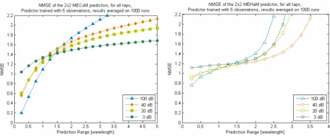
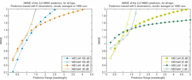
9.4.3 Using 5 observations on 2x2 MIMO ...52
9.4.4 Improving MEHaM ...52
9.5 TESTING 4X4MIMO SCENARIOS... 54
9.5.1 Noise free conditions on 4x4 MIMO...55
9.5.2 Adding coloured noise...55
9.5.3 Improving MEHaM in 4x4 scenarios ...56
9.6 CONCLUSIONS ABOUT MIMO COMPUTATIONS... 58
10 WORKING WITH QUANTIZED VALUES ... 60
10.1 QUANTIZATION LAW... 60
10.2 INFLUENCE ON 2X2MIMO PREDICTORS... 61
10.3 INFLUENCE ON 4X4MIMO PREDICTORS... 62
File: SURFACE_D2_2_v2_0.doc, January 2007 Page 6 of 86
11 AN INOVATIVE MIMO CHANNEL PREDICTOR... 65
11.1 WORKING SCHEME OF THE PREDICTORS... 65
11.2 CHOICE OF THE MATRIX CONTAINING CHANNEL INFORMATION... 65
11.3 COMPUTATION OF THE POLES... 66
11.4 SUMMARY ALGORITHM... 67
11.5 NUMERICAL COMPLEXITY OF THE NEW MIMO PREDICTOR... 68
11.6 PERFORMANCES OF THE NEW MIMO PREDICTOR... 68
12 PREDICTIONS ON THE RANK OF THE MIMO CHANNEL MATRIX ... 72
12.1 2X2MIMO SCENARIOS... 72
12.2 4X4MIMO SCENARIOS... 75
12.3 USING ANOTHER QUANTIZATION LAW... 76
12.4 CONCLUSIONS ON RANK PREDICTION... 81
13 REFERENCES ... 83
14 CONCLUSIONS... 84
File: SURFACE_D2_2_v2_0.doc, January 2007 Page 7 of 86
LIST OF FIGURES
FIGURE 3-1:URBAN MICRO ENVIRONMENT, POSITION OF BS AND MS... 16
FIGURE 3-2:URBAN MICRO ENVIRONMENT, ASSESSMENT ON POSITION OF BS AND MS ... 16
FIGURE 4-1:PREDICTIONS OF THE POLYNOMIAL ESTIMATOR... 22
FIGURE 6-1:A PLOT EXAMPLE OF COMPUTED POLES (GREEN PLOTS).THE GREEN CIRCLE IS THE UNITARY CIRCLE, AND THE RED CURVE STANDS FOR THE THRESHOLD... 32
FIGURE 7-1:A SAMPLE RESULT OF THE SISO PREDICTORS (E=14)... 35
FIGURE 7-2:ANOTHER SAMPLE RESULT OF THE SISO PREDICTORS (E=14)... 35
FIGURE 7-3:MORE SAMPLE RESULTS OF THE SISO PREDICTORS (E=14)... 36
FIGURE 7-4:SAMPLE RESULT OF OUR SISO PREDICTORS (E=20). ... 36
FIGURE 7-5:A RESULT SAMPLE OF OUR SISO PREDICTORS... 37
FIGURE 7-6:THE SAME RESULT SAMPLE OF OUR SISO PREDICTORS AS IN THE FIGURE ABOVE, WITH NORMALIZED POLES, FOR THE ANDERSEN ET AL. PREDICTOR... 37
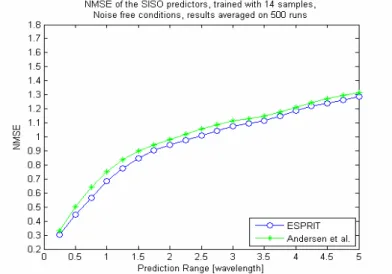
FIGURE 7-7:TIME EVOLUTION OF THE NMSE FOR THE SISO PREDICTORS IN NOISE FREE CONDITIONS (E =14) .. 38
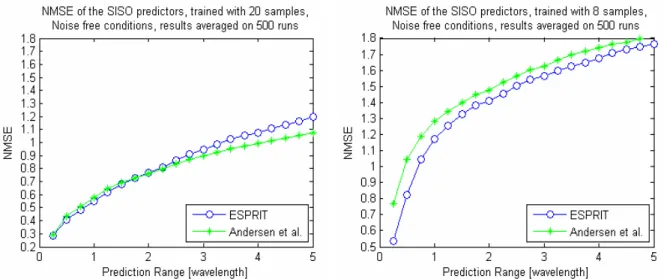
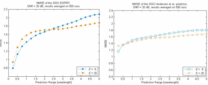
FIGURE 7-8:TIME EVOLUTION OF THE NMSE FOR THE SISO PREDICTORS IN NOISE FREE CONDITIONS(E =20 AND E =8) ... 39
FIGURE 7-9:TIME EVOLUTION OF THE NMSE FOR THE SISO PREDICTORS, NOISE FREE CONDITIONS... 39
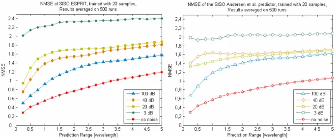
FIGURE 7-10:TIME EVOLUTION OF THE NMSE FOR OUR PREDICTORS IN NOISY SITUATIONS (E=20) ... 40
FIGURE 7-11:TIME EVOLUTION OF THE NMSE FOR OUR PREDICTORS IN NOISY SITUATIONS (E=8) ... 40
FIGURE 7-12:INFLUENCE OF THE NUMBER OF OBSERVATIONS IN NOISY CONDITIONS (SNR=20 DB) ... 41
FIGURE 9-1:A TYPICAL MECOM COMPUTATION... 45
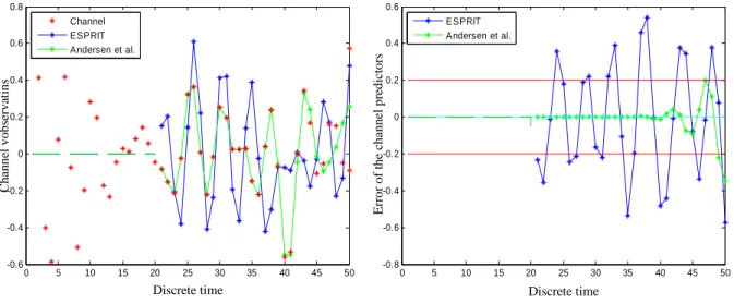
FIGURE 9-2:ERROR OF A TYPICAL MIMOESPRIT COMPUTATION... 46
FIGURE 9-3:A TYPICAL MIMOANDERSEN ET AL. PREDICTOR COMPUTATION... 46
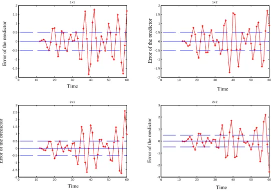
FIGURE 9-4:ERROR OF A TYPICAL MIMOANDERSEN ET AL. PREDICTOR COMPUTATION... 47
FIGURE 9-5:TIME EVOLUTION OF THE NMSE OF OUR MIMO PREDICTORS IN NOISE FREE CONDITIONS... 48
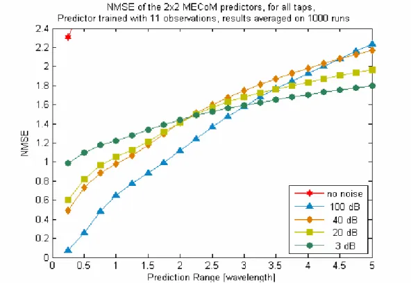
FIGURE 9-6:TIME EVOLUTION OF THE NMSE FOR MECOM IN NOISY SITUATIONS (E=11)... 49
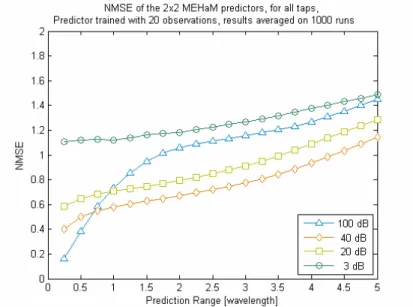
FIGURE 9-7:TIME EVOLUTION OF THE NMSE FOR MEHAM IN NOISY SITUATIONS (E=11) ... 50
FIGURE 9-8:RELIABILITY OF OUR TWO MIMO PREDICTORS (E=11,SNR=40 DB OR 3 DB) ... 50
FIGURE 9-9:TIME EVOLUTION OF THE NMSE FOR MECOM IN NOISY SITUATIONS (E=20)... 51
FIGURE 9-10:TIME EVOLUTION OF THE NMSE FOR MECOM IN NOISY SITUATIONS (E=20)... 51
FIGURE 9-11:TIME EVOLUTION OF THE NMSE FOR MECOM AND MEHAM IN NOISY SITUATIONS (E=5)... 52
FIGURE 9-12:INFLUENCE OF THE NUMBER OF COLUMNS ON THE MEHAM PREDICTOR (5 OBS,SNR=3,20,100 DB) ... 53
FIGURE 9-13:COMPARISON BETWEEN MECOM AND MEHAM, INFLUENCE OF THE LIMITED NUMBER OF COLUMNS ON MEHAM, AT SEVERAL NOISE LEVELS (E=5)... 54
FIGURE 9-14:TIME EVOLUTION OF THE NMSE FOR THE 4X4MIMO PREDICTORS, IN NOISE FREE CONDITIONS (E=17 AND 33)... 55
FIGURE 9-15:TIME EVOLUTION OF THE NMSE FOR THE 4X4MIMO PREDICTORS, NO LIMITATION ON THE NUMBER OF COLUMNS FOR MEHAM, WITH ADDITIVE GAUSSIAN NOISE (E=17)... 55
FIGURE 9-16:INFLUENCE OF THE NUMBER OF COLUMNS ON THE 4X4MEHAM PREDICTOR (17 OBS,SNR=3,20DB) 56 FIGURE 9-17:INFLUENCE OF THE NUMBER OF COLUMNS ON THE 4X4MEHAM PREDICTOR (17 OBS,SNR=40,100DB) ... 57
FIGURE 9-18:COMPARISON BETWEEN MECOM AND MEHAM IN 4X4MIMO SCENARIO, INFLUENCE OF THE LIMITED NUMBER OF COLUMNS ON MEHAM, AT SEVERAL NOISE LEVELS (E=17)... 58
File: SURFACE_D2_2_v2_0.doc, January 2007 Page 8 of 86
FIGURE 10-1:QUANTIZATION LAW, USING 3 OR 6 BITS... 60
FIGURE 10-2:INFLUENCE OF QUANTIZATION ON 2X2MIMO CHANNEL,SNR=3 DB... 61
FIGURE 10-3:INFLUENCE OF QUANTIZATION ON 2X2MIMO CHANNEL,SNR=20 DB... 61
FIGURE 10-4:INFLUENCE OF QUANTIZATION ON 2X2MIMO CHANNEL,SNR=100 DB... 62
FIGURE 10-5:INFLUENCE OF QUANTIZATION ON 4X4MIMO CHANNEL,SNR=3 DB... 63
FIGURE 10-6:INFLUENCE OF QUANTIZATION ON 4X4MIMO CHANNEL,SNR=20 DB... 63
FIGURE 10-7:INFLUENCE OF QUANTIZATION ON 4X4MIMO CHANNEL,SNR=100 DB... 64
FIGURE 11-1: COMPUTATION OF THE POLES, INFLUENCE OF THE PARAMETERS (4X4MIMO,SNR=20 DB,750 RUNS).. 67
FIGURE 11-2:EFFECTS OF QUANTIZATION ON 2X2 AND 4X4MIMO CHANNELS WITH SNR=3 DB ... 68
FIGURE 11-3:EFFECTS OF QUANTIZATION ON 2X2 AND 4X4MIMO CHANNELS WITH SNR=20 DB ... 69
FIGURE 11-4:EFFECTS OF QUANTIZATION ON 2X2 AND 4X4MIMO CHANNELS WITH SNR=100 DB ... 69
FIGURE 11-5:FLOATING POINT QUANTIZATION LAW, USING 6 BITS... 70
FIGURE 11-6:EFFECTS OF FLOATING POINT QUANTIZATION ON 2X2 AND 4X4MIMO CHANNELS WITH SNR=3 DB... 71
FIGURE 11-7:EFFECTS OF FLOATING POINT QUANTIZATION ON 2X2 AND 4X4MIMO CHANNELS WITH SNR=20 DB.... 71
FIGURE 11-8:EFFECTS OF FLOATING POINT QUANTIZATION ON 2X2 AND 4X4MIMO CHANNELS WITH SNR=100 DB.. 71
FIGURE 12-1:RANK PREDICTION OF 2X2MIMO CHANNEL (SNR=20 DB, QUANTIZATION ON 2X 6 BITS) ... 72
FIGURE 12-2:RANK PREDICTION OF 2X2MIMO CHANNEL (SNR=20 DB, QUANTIZATION ON 2X 3 BITS) ... 72
FIGURE 12-3:RANK PREDICTION OF 2X2MIMO CHANNEL (SNR=20 DB, QUANTIZATION ON 2X 32 BITS) ... 73
FIGURE 12-4:RANK PREDICTION OF 2X2MIMO CHANNEL (SNR=20 DB, NO QUANTIZATION)... 73
FIGURE 12-5:RANK PREDICTION OF 2X2MIMO CHANNEL, WITH EACH TAP CONSIDERED SEPARATELY (SNR = 20 DB, QUANTIZATION ON 2X 6 BITS)... 74
FIGURE 12-6:RANK PREDICTION OF 4X4MIMO CHANNEL (SNR=20 DB, QUANTIZATION ON 2X 6 BITS) ... 75
FIGURE 12-7:RANK PREDICTION OF 4X4MIMO CHANNEL (SNR=20 DB, QUANTIZATION ON 2X 3 BITS) ... 75
FIGURE 12-8:RANK PREDICTION OF 4X4MIMO CHANNEL, WITH EACH TAP CONSIDERED SEPARATELY (SNR = 20 DB, QUANTIZATION ON 2X 6 BITS)... 76
FIGURE 12-9:FLOATING POINT QUANTIZATION LAW, USING 3 TO 6 BITS... 77
FIGURE 12-10:PREDICTION RANK OF 2X2MIMO CHANNEL, FLOATING POINT QUANTIZATION ON 2X 3 BITS (SNR =20 DB)... 77
FIGURE 12-11:PREDICTION RANK OF 2X2MIMO CHANNEL, FLOATING POINT QUANTIZATION ON 2X 4 BITS (SNR =20 DB)... 77
FIGURE 12-12:PREDICTION RANK OF 2X2MIMO CHANNEL, FLOATING POINT QUANTIZATION ON 2X 5 BITS (SNR =20 DB)... 78
FIGURE 12-13:PREDICTION RANK OF 2X2MIMO CHANNEL, FLOATING POINT QUANTIZATION ON 2X 6 BITS (SNR =20 DB)... 78
FIGURE 12-14:PREDICTION RANK OF 4X4MIMO CHANNEL, FLOATING POINT QUANTIZATION ON 2X 3 BITS (SNR =20 DB)... 79
FIGURE 12-15:PREDICTION RANK OF 4X4MIMO CHANNEL, FLOATING POINT QUANTIZATION ON 2X 4 BITS (SNR =20 DB)... 79
FIGURE 12-16:PREDICTION RANK OF 4X4MIMO CHANNEL, FLOATING POINT QUANTIZATION ON 2X 5 BITS (SNR =20 DB)... 79
FIGURE 12-17:PREDICTION RANK OF 4X4MIMO CHANNEL, FLOATING POINT QUANTIZATION ON 2X 6 BITS (SNR =20 DB)... 80
FIGURE 12-18:PREDICTION RANK OF 2X2MIMO CHANNEL, FLOATING POINT QUANTIZATION ON 2X 4 BITS (SNR =3 DB)... 80
FIGURE 12-19:PREDICTION RANK OF 4X4MIMO CHANNEL, FLOATING POINT QUANTIZATION ON 2X 4 BITS (SNR =3DB)... 80
FIGURE 12-20:PREDICTION RANK OF 2X2MIMO CHANNEL, FLOATING POINT QUANTIZATION ON 2X 4 BITS (SNR =100 DB)... 81
FIGURE 12-21:PREDICTION RANK OF 4X4MIMO CHANNEL, FLOATING POINT QUANTIZATION ON 2X 4 BITS (SNR =100 DB)... 81
File: SURFACE_D2_2_v2_0.doc, January 2007 Page 9 of 86
LIST OF SYMBOLS
• nT- number of transmit antennas
• nR- number of receive antennas
• nSamples - number of time samples considered by the SURFACE channel model
• nSub - number of subcarriers considered by the SURFACE channel model
• nSymb - number of symbols per PRB
• nTaps - number of taps considered by the SURFACE channel model
• mn
h - SISO component of a MIMO channel, relevant for the link from the mth transmitting antenna to the nth receiving one.
• mn
hˆ - predicted value of hmn
• ak - amplitude for the k
th
path
•
φ
k - spatial Doppler shift for the kth
path
•
τ
k - tap delay for the kth
path
•
θ
k - angle between the motion of the receiver and the direction of waves impingingfrom the kth scatterer
• Ns- number of scatterers local to the receiver (and consequently, the number of NLOS
paths) • λπ λ 2 =
k - wave number, where λ is the wave length
• j k
k e
z = φ - signal poles
• Φ - diagonal matrix containing the signal poles
• Z - Vandermonde matrix containing the signal poles
• R - correlation matrix of the channel
• x(t) - transmitted signal
• y(t) - received signal
• w(t) - additive noise
• D - degree of the polynomial estimator
• E - number of observations used to compute a predictor
• H - n×mHankel matrix containing the channel observations
File: SURFACE_D2_2_v2_0.doc, January 2007 Page 10 of 86
• #
. - Pseudo inverse matrix operator • . - Conjugate transpose matrix operator * •
.
- Complex conjugate matrix operator• .UP - Matrix operation, removes the last row of a matrix
• .DOWN - Matrix operation, removes the first row of a matrix
File: SURFACE_D2_2_v2_0.doc, January 2007 Page 11 of 86
LIST OF ACRONYMS
• 3GPP 3rd Generation Partnership Program
• CPU Central Processing Unit
• CSI Channel State Information
• ESPRIT Estimation of Signal Parameters by Rotational Invariance Techniques
• IST Information Society Technologies
• LOS Line-of-sight
• MECoM MIMO ESPRIT based on Correlation Matrix
• MEHaM MIMO ESPRIT based on Hankel Matrix
• MIMO Multiple Input Multiple Output
• MISO Multiple Input, Single Output
• NMSE Normalized Mean Square Error
• NLOS Non Line Of Sight
• PRB Physical Resource Block
• QoS Quality of Service
• ROMANTIK ResOurce Management and AdvaNced Transceiver algorIthms for
multihop networKs
• Rx Receiving antenna
• SCM Spatial Channel Model
• SCME Spatial Channel Model Extended
• SISO Single Input Single Output
• SNR
( )
( )
2 2 10 10 Ratio Noise to Signal w mean h mean log ≡ ; in decibels (dB)• SURFACE Self Configurable Air Interface
• SVD Singular Value Decomposition
• TDD Time Division Duplex
• Tx Transmitting antenna
File: SURFACE_D2_2_v2_0.doc, January 2007 Page 12 of 86
1 INTRODUCTION
Multiple Input Multiple Output (MIMO) technologies are now really attractive because of their benefits: using several antennas both on transmitter and receiver sides can improve the amount of transmissible information if there is sufficient decorrelation between the antenna pairs. These benefits will be useful to propose new wireless multimedia services, because they require good quality channels, with high data rates.
To properly exploit time varying wireless channel, the transmitter needs to collect knowledge about the channel state, to use the right power level to transmit, or to wait a bit if the channel can not accept information currently, but in TDD modes. The transmitter can not collect knowledge about the state of the channel, unless the receiver feeds back some information. However, when the transmitter receives the Channel State Information (CSI) fed back by the receiver, this CSI can be outdated… So to evaluate the current channel state, the transmitter shall make “guesses”, to predict the channel state. Hence, this is the reason why predictions are so useful in wireless communication.
In this deliverable, we aim at extending existing SISO1 and MIMO simplified channel models in order to design a MIMO predictor of the channel state.
First, we will present the WINNER’s SCME channel model. WINNER2 is a European project [WIN], and it has implemented SCME in Matlab; which is an extension of the 3GPP Spatial Channel Model. We will use it to provide us reference CSI for our computer simulations. We will then present the SURFACE channel model, which is a wrapper of the WINNER’s SCME, where we updated a few parameters to match other SURFACE workpackages requirements.
An overview of relevant channel models and predictors will follow. Two of them revealed particularly interesting and appropriate for our working objectives. They are both based upon the ESPRIT4 algorithm. We will detail them, and explain their mathematical background. Following this description, we will give results of computations about these two predictors. Actually, these two predictors are only SISO predictors, so we will extend them into MIMO predictors, and then present some computation results. We will also investigate the robustness against limited feedback quantization used to train the MIMO predictors.
We will then merge the two predictors into a single one, using best of both techniques, and present its performance.
Finally, we will investigate the topic of rank prediction of the MIMO channel matrix. Actually, the whole matrices will be predicted by the MIMO predictor, and then their rank will be assessed.
The document ends with concluding remarks and future work items.
1 Single Input Single Output 2
Wireless World Initiative New Radio
File: SURFACE_D2_2_v2_0.doc, January 2007 Page 13 of 86
2 THE WINNER’S CHANNEL SIMULATOR
This section shortly introduces the WINNER’s SCME, a comprehensive spatial channel model we will use as reference during our Matlab computations.
WINNER is a European project, from the Sixth Framework Program effort [WIN]. Among its numerous contributions, it extended the 3GPP Spatial Channel Model (SCM) into a new model called SCME [Bau 05], [SCM 05].
The original SCM is a ray-based MIMO channel model, with a stochastic modeling of the scatterers. It is divided into several environment scenarios, both line-of-sight (LOS) and non-LOS. It models the received signal as 6 distinct delay paths (channel taps), and each one is the sum of 20 complex sinusoids. All the parameters (paths’ power, delay and angle of arrival/departure) are modeled as random variables, depending on given probability density and cross-correlations functions.
The main extensions brought by SCME are new environment scenarios and bandwidth of 100 MHz in both 2 and 5 GHz carrying frequencies, instead of only 5 MHz at 2 GHz.
The SCME channel model has been implemented in Matlab. Given the environment scenario and the antenna array configurations, it generates channel matrices, then multidimensional arrays containing a specified number (100 per default) channel impulse response samples for all links.
Here are the default parameters of SCME:
• 2 Tx, 2 Rx, 6 paths per Tx-Rx pair (so 2 x 2 MIMO channel, with 6 taps); • Urban Micro scenario;
• Mobile user velocity: 10 m/s ;
• Sampling : 2 samples per half wavelength,
so ∆t=3.75 ms=7.5 TTI (with LTETTI=0.5ms); • 100 time samples are computed;
• Center frequency: 2 GHz.
The resulting multidimensional array has therefore 2 x 2 x 6 x 100 dimensions.
For the purpose of the present work, we will feed our predictors with the channel impulse response samples produced by SCME.
To match other workpackages requirements, the WINNER’s SCME has been tuned. The next section presents the modifications we made on the channel model
File: SURFACE_D2_2_v2_0.doc, January 2007 Page 14 of 86
3 THE SURFACE CHANNEL MODEL
This section presents the SURFACE channel model, which is a wrapper to 3GPP Spatial Channel Model Extended (SCME) implementation provided by FP7 IST WINNER project v1.0 (May 30, 2005) [SCM 05]. Either existing SCME parameters or a few new ones are set in accordance with FP7 IST SURFACE D7.3 [SD 7.3].
Two main scenarios have been implemented, namely Micro-cell and Pico-cell scenarios, both for urban area. The Micro-cell scenario is derived from the 3GPP Micro cell scenario [3GPP 07], and proposes the choice between Outdoor to Outdoor and Outdoor to Indoor alternatives. The Pico-cell scenario is derived from the B1 scenario of the WINNER II IST project [WIN 6.13.7] and is only for outdoor-to-outdoor, with both LOS and NLOS coverage. Two modeling levels are proposed. The model can be run at link level, and perform simulations at PRB scale, or it can be run at system level where the whole channel bandwidth is considered and no pathloss nor shadowing is applied.
3.1 Input/Output parameters
The SURFACE channel model has been implemented as a MATLAB function with 5 input parameters, and 3 output parameters.
The input parameters are
1. The computation level : “link” or “system”;
2. The scenario : “micro_o2o”, “micro_o2i”, “pico_los” or pico_nlos”; 3. The terminal velocity, in km/h;
4. The number of transmit antennas; 5. The number of receive antennas;
The outcomes of the model depend on the level. Please note that there are three output variables, whether this is a link- or a system-level simulation. However, the meaning of these output variables differs.
For the link level, the output parameters are:
1. The MIMO channel matrix (channel response), where nT is the number of Tx, n R is the number of Rx, nSub is one (channel is computed for the full PRB, and not for each of its subcarriers), and finally nSymb is the number of symbols of a PRB;
2. C is a flag set up at 1 because we emulate one channel matrix per PRB; 3. T is a flag set up at 0 (no time compression).
File: SURFACE_D2_2_v2_0.doc, January 2007 Page 15 of 86 For the system level, the output parameters are:
1. The MIMO channel matrix, with size nT xnRxnTapsxnSamples, where nT is the number of Tx, n R is the number of Rx, nTaps is the number of taps (6 actually), and finally
Samples
n is the number time samples; 2. The channel covariance matrix;
3. A structure containing the delays and the powers of each tap, and some other parameters.
3.2 Remarks about the model
For link-level simulations, setting SCME parameters for typical PRB bandwidths leads to a non frequency selective channel. This is why subcarrier scale is useless, and we model the channel at PRB scale.
Still for link-level simulations, the carrier frequency is hard coded to the one of a PRB chosen randomly in the bandwidth of the channel. In Micro-Cell scenarios, there is a total of 50 PRBs in a 10 MHz bandwidth, whereas in Pico-Cell scenarios, there are 60 PRBs in a 20 MHz bandwidth.
For system-level simulations, SCME is hard coded to provide the channel model of a single link (one MS, one BS, whatever the number of antennas). It could however deliver such models for several links simultaneously.
WINNER B4 model is currently not supported in the Pico-Cell NLOS indoor MS scenario.
3.3 Pathloss assumptions
For Pico-cell scenario, the pathloss has been adapted, because it requires some parameters SCME does not have. According to [SD 7.3, Table 7-1], for LOS case, pathloss should be
[ ]
[ ]
bpLOS d m f GHz d R
PL =22.7log10( 1 )+41+20log10( /5), 1<
[ ]
bp[ ]
bpLOS d m R f GHz d R
PL =40log10( 1 )+41−17.3log10( )+20log10( /5), 1≥
with λ ) )( ( 1 1 4 − − = BS MS bp h h R and d1=10m...5km
and for NLOS case, pathloss should be
[ ]
) 20 12.5 10 log ([ ]
) (d1m n n 10 d2 m PLPLNLLOS = LOS + − j+ j
with nj =max(2.8−0.0024*d1
[ ]
m, 1.84) and d2 =w/2...2km, w=15mFile: SURFACE_D2_2_v2_0.doc, January 2007 Page 16 of 86 BS d1 d2 o MS d
Figure 3-1 : Urban micro environment, position of BS and MS
Actually, WINNER SCME only provides us with distance d, and no angles to derive distances
d1 and d2. So we imposed the following scheme to estimate the desired distances d1 and d2,
where angle θ worth 45° in NLOS case, or 6.4° in LOS case (if d=100m, θ = 6.4° implies d1=
90m and d2=10m) :
Figure 3-2 : Urban micro environment, assessment on position of BS and MS
The micro-cell pathloss has also been changed from the SCME settings, to match LTE pathloss assumption, according to [SD 7.3, Table 4-1], but it only depends on distance d, which value is known by SCME. So the LTE pathloss did not require any special assumption, unlike the WINNER II B1 pathloss of pico-cell scenarios.
The next two subsections details the parameters of the channel model, for each scenario. Then we will move to channel prediction and review a limited set of channel models and prediction strategies that revealed relevant for our prediction work.
d BS MS d1 d2 θ
File: SURFACE_D2_2_v2_0.doc, January 2007 Page 17 of 86
3.4 Link level parameters
Micro-Cell Pico-Cell
Parameters
Outdoor-to-outdoor
Outdoor-to-indoor LOS NLOS
Source
Level ‘link’ -
Scenario ‘micro_o2o’ ‘micro_o2i’ ‘pico_los’ ‘pico_nlos’ - Velocity [km/h] 3/30 nT User-defined User-defined input parameters nR User-defined Channel C 1 1 1 1 Output variables T 0 0 0 0 Internal SURFACE requirements following October 28, 2007 conference call Carrier frequency [GHz] Depends on simulated PRB, within [1.75 ; 2.25] Depends on simulated PRB, within [4.6 ; 5.4] TS 36.211 v8.0.0 MS-BS distance Random Original SCME MS height [m] 1.5 Original SCME BS height [m] 15 10 D7.3, Table 4-3 Number of paths in TDL 1 SCME flat over a PRB Delay sampling [µs] 5.67 (= 1/180 kHz) 3.2 (= 1/312.5 kHz) - Number of time samples 14 symbols or 1 ms 12 symbols or 0.3456 ms D7.3, Table 2-1 Time sampling [µs] 71.42 28.8 D7.3, Table 2-2 WINNER scenario B1 Pathloss D7.3, Tables 4-1 and 4-2 Internal SCME parameters Shadowing
File: SURFACE_D2_2_v2_0.doc, January 2007 Page 18 of 86
3.5 System level parameters
Micro-Cell Pico-Cell
Parameters
Outdoor-to-outdoor
Outdoor-to-indoor LOS NLOS
Source
Level ‘system’ -
Scenario ‘micro_o2o’ ‘micro_o2i’ ‘pico_los’ ‘pico_nlos’ - Velocity [km/h] 3 nT User-defined User-defined input parameters nR User-defined Channel C Covariance matrix Output variables T SCME’s FullOutput Internal SURFACE requirements following October 28, 2007 conference call Carrier frequency [GHz] 2 5 MS-BS distance Random MS height [m] 1.5 BS height [m] 15 10 D7.3, Table 4-3 Number of paths in TDL 6 Delay sampling [µs] 100 50 Number of time samples 100 Time sampling [ms] 135 54 WINNER scenario B1
Pathloss No pathloss from SCME (PathLossModelUsed = ‘no’)
Internal SCME parameters
Shadowing No shadowing from SCME (ShadowingModelUsed = ‘no’)
File: SURFACE_D2_2_v2_0.doc, January 2007 Page 19 of 86
4 MODELISATION AND PREDICTION - STATE OF ART
In this section, we will present some channel models and estimators we investigated. There are many more existing channel models, but we are limiting our scope to the ones that have been showed to perform predictions. We will first review the ROMANTIK parametric model and a polynomial estimator. Then we will go through a MISO estimator, and we will end this section with an ESPRIT-based technique, which seems to fit well into our approach.
Before introducing these models, we will say a word about Kalman filters. This kind of filters would be very useful to help our models and predictors to deal with noisy situations. Indeed, Kalman filters could perform smoothing to remove the effects of the noise and provide a better estimate of the channel state. But the main drawback of these filters is that they need significant computational power. We are rather aiming at designing a predictor which can be run on typical energy- and CPU-limited devices. In a word, we are looking for the best trade-off between prediction performance and computer requirements. So we will not discuss Kalman filters further on.
4.1 The ROMANTIK model
ROMANTIK is an FP5 IST project. Its name means ResOurce Management and AdvaNced Transceiver algorIthms for multihop networKs. As part of its contributions, it proposed a
channel model. The ROMANTIK model was initially a SISO parametric model [Bar 03a]. It has later been generalized into a MIMO model [Bar 03b]. These models also perform prediction of the channel state. It is worthwhile mentioning here that the ongoing FP6 IST project URANUS1 follows up ROMANTIK activities, in working towards a parametric model of channel estimation.
4.1.1 The SISO model
Here is the SISO channel model, from [Bar 03a], where the channel h depends on time t and delay
τ
This model contains 3
(
Ns+1)
parameters: ak, τk, φk ∀k. The ak are the amplitudes, thek
τ are the delays and the φk are the Doppler frequency shifts of each path of the channel. Actually, it’s a
(
Ns+1)
-order model; a sum of(
Ns +1)
weighted complex sinusoids. Toestimate these parameters, sounding is suggested in [Bar 03a].
Hence for the prediction, the scheme is first to estimate the 3
(
Ns +1)
parameters of the channel, then to run the model with the estimated parameters to predict future values. Because these parameters are time-varying, predictions will remain reliable only for a limited period of time. The prediction at time t+∆hence writes:
1 Universal RAdio-liNk platform for efficient USer centric access
) ( , k( t) N k t j k s k e a t h τ ) =
∑
φ δ τ −τ + = ( 1 1 ) ( , ˆ ) ( ) ∆ + + = ∆ + − = ) ∆ +∑
k t N k t j k s k e a t h(τ
φδ
τ
τ
1 1 (File: SURFACE_D2_2_v2_0.doc, January 2007 Page 20 of 86
4.1.2 The MIMO model
ROMANTIK further proposed a MIMO channel model ([Bar 03b]), considering that a
R T n
n × MIMO channel can be regarded as nT ⋅nRspatially correlated SISO channels.
The exploitation of the spatial correlation lead ROMANTIK to assume that the delays
τ
k and the Doppler shiftsφ
k are identical for all the nT⋅nRSISO components of a given MIMO channel. This assumption is motivated by the fact that antennas are relatively close with respect to the distance between the transmitter and the receiver, such that the variation of delay or Doppler shift from an antenna pair to another can be regarded as negligible.Indeed, the delays depend on the path lengths, and in front of the distance between the transmitter and the receiver, the few centimeters between transmit/receive antennas are quite negligible. The same applies to the Doppler shifts. They depend on the angle between the movement of the receiver and the direction of the waves impinging from the scatterers. If the scatterers are not too close, the variations of angle between receiving antennas are negligible too. However, despite delays and Doppler shifts are identical from one spatial link to the other, those links can appear uncorrelated due to the difference between their amplitudes. In the ROMANTIK MIMO channel model, the communication link between the mth transmitting antenna and the nth receiving one is given by:
)
(
,
k( t) N k t j k n mt
sa
e
kh
τ
)
=
∑
φδ
τ
−
τ
+ =(
1 1 n mThe prediction scheme is the same than in the SISO case: first estimate the parameters of the channel model by sounding, then run it to compute future values. For a given link, the MIMO prediction at time t+∆writes:
)
(
,
ˆ
) ( ) ∆ + + = ∆ +−
=
)
∆
+
∑
k t N k t j k n m s ke
a
t
h
(
τ
φ
δ
τ
τ
1 1 ( n m 4.1.3 CommentsAs we can see, ROMANTIK relies on a parametric model. From a feedback point of view, a parametric model has the advantage to be fully defined with a reduced set of parameters. Indeed, it’s easier to send a small amount of parameters than a lot of CSI. On the other hand, the predictions will remain reliable as long as the parameters remain constant.
The core of this parametric model is actually to estimate these parameters. To perform it, ROMANTIK suggest sounding, and documents [Bar 03a] and [Bar 03b] describe in details several sounding schemes.
As we do not know whether SURFACE will afford sounding, we considered other options. In the next section, we will review a simpler predictor, because it is polynomial.
File: SURFACE_D2_2_v2_0.doc, January 2007 Page 21 of 86
4.2 A Polynomial Estimator
4.2.1 Proposed scheme
This section is based on [Che 03]. The authors propose first to compute a polynomial model which fits a set of channel observations, then to run this model in order to predict future channel observations. In fact, the model is split into two separate models, one for the real part of the channel state, and the other for its imaginary part.
The polynomial, discrete time channel model, including an initial phaseϕk, writes:
)
(
.
)
(
)
(
n
a
e
( )I
n
j
Q
n
h
j kn k k2 1 N 1 k s
+
=
=
+ + =∑
πφ ϕWe have to compute the two polynomials I(n) and Q(n) such that
( )
(
)
≡ ℜ = ⋅ =∑
− = n h n c n I D k k k 1 0 )( Real part of the channel state
( )
(
)
≡ ℑ = ⋅ =∑
− = n h n d n Q D k k k 1 0 )( Imaginary part of the channel state
where D is the degree of the polynomial. Therefore, to derive the ck and the dk, we have to solve these linear systems:
(
)
(
)
(
)
1
1
1
1
1
1
1
1
1
1 1 0 1 1
+
−
ℜ
−
ℜ
ℜ
=
−
−
− − −)
(
)
(
)
(
D
n
h
n
h
n
h
c
c
c
)
(D
D
D
D
D D DM
M
L
M
O
M
M
K
L
;(
)
(
)
(
)
1
1
1
1
1
1
1
1
1
1 1 0 1 1
+
−
ℑ
−
ℑ
ℑ
=
−
−
− − −)
(
)
(
)
(
D
n
h
n
h
n
h
d
d
d
)
(D
D
D
D
D D DM
M
L
M
O
M
M
K
L
.More details about mathematical justification of the algorithm is given in [Che 03].
The predictions, l time instants later, are then given by:
∑
− = + = + 1 0 ) ( ) ( D k k k D l c l n Î and∑
− = + = + 1 0 ) ( ) ( ˆ D k k k D l d l n Q .∑
− = + ⋅ + = + ⇒ 1 0 ) ( ) i ( ) ( ˆ D k k k k d D l c l n hFile: SURFACE_D2_2_v2_0.doc, January 2007 Page 22 of 86
4.2.2 Comments
This polynomial channel model is very simple, with only two small matrices to invert, which additionally are always the same. Their inverse could therefore be precomputed, which would ease the process.
The model is also very simple because it does not need a lot of observations. We can aim at using polynomials with degree 3, 5 or at least 10. It means that we do not need more than
E = 3, 5 or 10 observations to produce predictions, where E is the number of channel
observations the predictor needs.
However, there are two main drawbacks: predictions are only reliable on very short term and this is a SISO model.
4.2.3 Results of computations
We have implemented this predictor in a Matlab script, and tested it with WINNER’s SCME. SCME was used with its default values listed in Section 2. Figure 4-1 shows two
representative runs of the predictor (real part only). The left subfigure is obtained with a polynomial of degree 2, and the right one with a polynomial of degree 7. In the first case, the warm-up, which is the initial period until E channel observations have been collected, is only 3 observations. It is 8 in the second case. During the warm-up period, no prediction is yet available.
Figure 4-1 : Predictions of the polynomial estimator
These predictions are not reliable with D = 2, and its gets worse when increasing the degree of the polynomial.
This model is actually too simple and it can not perform well with a too low sampling rate as the one used in Figure 4-1. Therefore, it cannot predict the oscillations of the channel state, and its predictions often fall much below or above the value it has to predict, resulting in a significant prediction error.
We will now review a MISO1 estimator, which represents the channel as a sum of weighted sinusoids. It is not as simple as the polynomial estimator is. Hence, it should be more accurate.
1 Multiple Input Single Output.
0 5 10 15 2 0 2 5 3 0 3 5 40 4 5 5 0 -4 -3 -2 -1 0 1 2 3 4 5 S C M E C h an n e l E s t im a tion (M = 7 ) W A R M U P 0 5 10 15 2 0 2 5 3 0 3 5 40 4 5 5 0 -3 -2 -1 0 1 2 3 S C M E C h an n e l E s t im a tion (M = 2 ) W A R M U P
Discrete Time (in steps) Discrete Time (in steps)
C h an n el o b se rv at io n s C h an n el o b se rv at io n s (D=2) (D=7)
File: SURFACE_D2_2_v2_0.doc, January 2007 Page 23 of 86
4.3 A MISO estimator
This subsection is based on the predictor described in [Arr 02]. This predictor is meant to be used with smart antenna base stations, e.g. several (nT) transmitting antennas, and only one receiving antenna. This is a MISO channel model. This is the model, with the l index standing for the transmitting antenna this ‘‘sub-channel’’ is related with:
k s t j N k l k l
e
a
t
h
φ 1 1∑
+ ==
)
(
As mentioned above, the channel model is a weighted sum of complex sinusoids. With the help of mathematical properties detailed in [Arr 02], it can be expressed as a weighted sum of itself at past instants:
∑
+ = − = 1 1 s N k l k l k t h b t h ( ) ( )such that we just have to compute the bk, to be able to predict future channel observations from a linear combination of past values. To derive the bk, one has to solve a huge linear system, with the pseudo inverse of a large matrix to compute. More details about this predictor and the way to compute the bk coefficients are to be found in [Arr 02].
To exploit the spatial correlation between the nTchannels, the authors of [Arr 02] suggest to
use the same bk coefficients for each transmitting antenna.
To draw a conclusion about this method, we can say that it seems complex. It deals with larger matrices, which contain future measurements. The non causality of the method and the heavy computations motivated our choice not to test it.
We will now shortly present a channel model which seems us to be really promising. The next two sections will dig deeper into this SISO channel model and the MIMO model we have derived from it.
4.4 The Andersen et al. predictor
This last subsection is based on the paper [And 99]. Its authors model the channel as follows:
. , ) (t a e a z z e k h k s k s j k t k N k k t j N k k = = ∀ =
∑
∑
+ = + = 1 1 1 1 φ φIt means that the channel impulse response h(t) is considered as a weighted sum of
(
Ns +1)
complex sinusoids. The ak are the weighting coefficients and the φk are the spatial Dopplerfrequencies. So, the main goal of this method is to find the zk, called signal-poles, and the ak (amplitudes).
File: SURFACE_D2_2_v2_0.doc, January 2007 Page 24 of 86 Actually, this model can be seen as a modified version of the ESPRIT technique1. We performed Matlab computations with this channel model and it seems to work great with WINNER’s SCME. So we have investigated it deeper,
The next two sections provide more details about the working scheme of this ESPRIT-based technique. In Section 6, we will review deeply the Andersen et al. predictor, but the next section will first review the original ESPRIT technique.
File: SURFACE_D2_2_v2_0.doc, January 2007 Page 25 of 86
5 THE ESPRIT PREDICTOR
This section will detail the working scheme of the ESPRIT method [Sto 05]. We will discuss about the channel model and its parameters, then we will give its mathematical background, and we will conclude this section with a summary algorithm.
5.1 Channel Model
This is the basic channel model we will use, depending on distance x:
) cos( ) ( k s x k i N k k e a x h
∑
λ θ + = = 1 1 ,whereNs is the number of scatterers, ak is the amplitude,
θ
k is the angle between the motionof the receiver and the direction of arrival of the received signal, k is the wave number, λ
depending on the wavelength (kλ =2π λ).
To reduce the problem of modeling the channel state to a classical frequency estimation problem, we will assume that velocity is constant (so constant sampling in time is constant sampling in space) and that amplitude variations may be neglected. We will also transform the model into a discrete time model.
So, we have ekλ∆xcos(θj), where ∆x is the move between two discrete time steps. Actually,
) cos( k x
kλ ∆
θ
is the spatial Doppler shift. We will write itφ
k. We will also write i kk e z = φ . Therefore, kn N k k n i N k k e a z a n h s k s
∑
∑
+ = + = = = 1 1 1 1 φ ) ( .For our predictions, we have to find the i k
k e
z = φ (so-called signal poles) and the ak (amplitudes). We will now discuss about a way to derive these parameters.
5.2 Basic idea
At first, we considerA , a E x Ns Vandermonde matrix such as
=
− − Ns s N s N i E i E i i i ie
e
e
e
e
e
φ φ φ φ φ φ ) ( ) (A
1 1 2 2 1 1 11
1
L
M
O
M
L
L
.Actually, A is linked to the channel matrix, because the i j
File: SURFACE_D2_2_v2_0.doc, January 2007 Page 26 of 86 Be JUP =
(
IE−1 ,(
0,K0)
T)
and JDOWN =(
(
0,K0)
T ,IE−1)
, where Ik-1 is the square (E-1) x (E-1) identity matrix. So JUP and JDOWN are (E-1) x E matrices such thatUP i E i E i i UP s N s N e e e e J A A ) ( ) ( ∆ − − = = ⋅ φ φ φ φ 2 2 1 1 1 1 L M O M L L , and DOWN i E i E i i i i DOWN s N s N s N e e e e e e J A A ) ( ) ( ∆ − − = = ⋅ φ φ φ φ φ φ L M O M L 1 1 1 1 2 2 .
Note that these matrices are (E-1) x Ns. Actually, AUP is the A matrix without its last row, and
ADOWN is A without its first row.
It’s easy to see that AUP⋅Φ=ADOWN means that
= Φ s N i i i e e e φ φ φ 0 0 2 1 O
5.3 The ESPRIT technique (mathematical background)
We will consider now the vector y(n) = h(n)⋅x(n)+w(n) which is the received signal from the channel to study; where x is the information to transmit, and w is the noise (n is
discrete time). Actually, because kn N k k z a n h s
∑
+ = = 1 1 )( , we have this matrix equation :
a E n n n h( , −1,K, − ) = A⋅ . So y(n) = A⋅a⋅x(n)+w(n) .
Be R the covariance matrix of the received signal, the * denotes the conjugate transpose of
the matrix.
{
y(n) y(n)*}
E{
A a x(n) x(n)* a* A*}
E{
w(n) w(n)*}
E R = ⋅ = ⋅ ⋅ ⋅ ⋅ ⋅ + ⋅{
( ) ( )* *}
; A* A P I whereP E a x n x n a R = ⋅ ⋅ + = ⋅ ⋅ ⋅ ⇒σ
2 ∆Please pay attention that we need the hypothesis that the noise is a white noise to write:
{
w n w n}
IE ( )⋅ ( )* = σ2
Notice too that we have to be in discrete time to compute our predictors, so in the matrices R, A, P, there are discrete time values.
File: SURFACE_D2_2_v2_0.doc, January 2007 Page 27 of 86 We will write l = rank(A⋅P⋅A*). In fact, l=Ns +1 , the number of paths.
Actually, A⋅P⋅A* has Ns+1 positives eigenvalues, and k -(Ns+1) zero eigenvalues. They are linked to the eigenvalues of R.
If we write λ~j for the eigenvalues of A⋅P⋅A*, and λjfor those of R, we have that
+ = ∀ + = ∀ + = E N j N j s s j j , , , , ~ K K 2 1 1 2 2
σ
σ
λ
λ
Now let’s make a Singular Value Decomposition (SVD) of the R matrix (a square E x E matrix). ( ) ⋅ ⋅ = + + * * G S G S R E N N s s λ λ λ λ O O 2 1 1 0 0
where S contains the eigenvectors of the Ns+1 greatest eigenvalues, and G contains the remaining eigenvectors. So . * * G G S S R E N N s s ⋅ ⋅ + ⋅ ⋅ = + + λ λ λ λ 0 0 2 0 0 1 1 1 O O Let’s calculate R⋅S: S R⋅ = O 123 I N S S S s = + ⋅ ⋅ ⋅ * 1 1 0 0
λ
λ
+ O 123 0 2 0 0 = + ⋅ ⋅ ⋅ G S G E Ns *λ
λ
= ⋅ +1 1 0 0 s N Sλ
λ
O ;(It’s because of the SVD: the eigenvectors are orthonormalised, and then S ⊥G.)
⋅ = ⋅ ⇒ +1 1 0 0 s N S S R
λ
λ
OBut because R also equals A⋅P⋅A* +
σ
2I, R⋅S also equals A⋅P⋅A*⋅S +σ
2S !S S P S R⋅ = ⋅ ⋅ ⋅ +
σ
2 ⇒ A A* Therefore, ⋅P⋅ ⋅S +σ
2S = A* A ⋅ +1 1 0 0 s N Sλ
λ
O ;File: SURFACE_D2_2_v2_0.doc, January 2007 Page 28 of 86 And then Λ ⋅ = − − ⋅ = ⋅ ⋅ ⋅ ∆ + S S S P s N 2 1 2 1 0 0 σ λ σ λ O A* A . So, S P S C C ⋅ = = Λ ⋅ ⋅ ⋅ ⋅ = ∆ − A A* A 14 24 4 341 C S = ⋅ ⇒ A and A = S⋅C−1.
Now remember that we proved that JUP⋅A⋅Φ=JDOWN⋅A. So, because A = S⋅C−1, 1 1 − − ⋅Φ = ⋅ ⋅Φ = ⋅ = ⋅ ⋅ ⋅ ⋅S C J J J S C JUP UP A DOWN A DOWN ;
And then JUP⋅S⋅C ⋅Φ⋅C = JDOWN ⋅S
∆ = − 43 42 1 D 1
Finally we have that SUP⋅D = SDOWN, where
≡
= J S
SUP UP (E-1) first rows of S, and
≡
= J S
SDOWN DOWN (E-1) last rows of S.
Because D = C−1⋅Φ⋅C, and C is nonsingular, D and Φ share the same eigenvalues. They are related by a similarity transformation. Their eigenvalues are actually the diagonal elements of Φ, i.e. eiΦ1,eiΦ2, K, eiΦNs, our signal poles. Therefore, to find the i k
k e
z = φ , we have to compute the SVD of R to derive S. From S we can get the D matrix, whose
File: SURFACE_D2_2_v2_0.doc, January 2007 Page 29 of 86
5.4 How to compute the correlation matrix R?
First, we have to fill H , a Hankel matrix with the received signal. Please note that we will
need E=m+n−1 observations to fill the matrix.
−
+
+
+
+
=
)
(
)
(
)
(
)
(
)
(
)
(
)
(
)
(
)
(
)
(
)
(
)
(
H
1
2
1
1
4
3
2
3
2
1
n
m
h
n
h
n
h
n
h
m
h
h
h
h
m
h
h
h
h
L
M
O
M
M
M
L
L
Then, we can get an estimation of R by computing m H* H⋅ . Indeed,