Improvement of the driving simulator control and comparison between driver-road-vehicule interaction in real and simulated environment

(1)

HAL Id: tel-03033387

https://tel.archives-ouvertes.fr/tel-03033387

Submitted on 1 Dec 2020

HAL is a multi-disciplinary open access

archive for the deposit and dissemination of sci-entific research documents, whether they are pub-lished or not. The documents may come from teaching and research institutions in France or abroad, or from public or private research centers.

L’archive ouverte pluridisciplinaire HAL, est destinée au dépôt et à la diffusion de documents scientifiques de niveau recherche, publiés ou non, émanant des établissements d’enseignement et de recherche français ou étrangers, des laboratoires publics ou privés.

comparison between driver-road-vehicule interaction in

real and simulated environment

Navid Ghasemi

To cite this version:

Navid Ghasemi. Improvement of the driving simulator control and comparison between driver-road-vehicule interaction in real and simulated environment. Signal and Image processing. Université Paris-Est; Università degli studi (Bologne, Italie), 2020. English. �NNT : 2020PESC2010�. �tel-03033387�

(2)

in cotutela con Università Paris-Est

DOTTORATO DI RICERCA IN

Ingegneria Civile, Chimica, Ambientale e dei Materiali

Ciclo XXXII

Settore Concorsuale: 08/A3 Infrastrutture e Sistemi di Trasporto, Estimo e Valutazione

Settore Scientifico Disciplinare: ICAR/04 Strade, Ferrovie ed Aeroporti

IMPROVEMENT OF THE DRIVER SIMULATOR CONTROL AND

COMPARISON BETWEEN DRIVER-ROAD-VEHICLE INTERACTION IN

REAL AND SIMULATED ENVIRONMENT

Presentata da:

Navid Ghasemi

Coordinatore Dottorato

Supervisore

Prof. Ing. LUCA VITTUARI

Prof. Ing. Andrea SIMONE

Supervisore

Prof. Ing. Hocine IMINE

Co-Supervisore

Dott. Ing. Claudio Lantieri Esame Finale anno 2020

(3)

(4)

1 Keywords:

Real-time vehicle simulation Motion cueing algorithm Surrogate safety measures Eye-tracking

(5)

(6)

1

List of Figures

Figure 1. Road Infrastructure management approach (D.Lgs 35) ... 19

Figure 2. Pyramid of Traffic Events (Hyden,1977) ... 21

Figure 3. Driver-Vehicle- Environment system ... 23

Figure 4. Driving Simulator Architecture and Connections ... 29

Figure 5. Visual cueing unit (View from the driver seat) ... 30

Figure 6. Vehicle Model sub systems ... 31

Figure 7. Vehicle Model Blocks ... 32

Figure 8.a. Vehicle Fixed Coordinate System; b. Earth Fixed Coordinate System. ... 33

Figure 9.a. Rolling effective radius; b. Forces acting on the wheel; c. contact and speed and angular speed... 34

Figure 10. Single-track lateral model (bicycle model) ... 36

Figure 11. Motion cueing algorithm implementation ... 37

Figure 12. Simulator cabin and motion cueing platform... 38

Figure 13. Classical Motion Algorithm for Translational Motion ... 39

Figure 14. Lead vehicle velocity profile ... 42

Figure 15. Allowed velocity and driver velocity profile ... 49

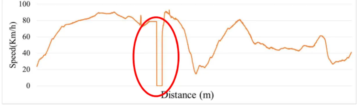
Figure 16. Velocity profile of one driver with a lost of GPS signal ... 50

Figure 17. a VBOX HD2 data recorder; b. IMU and GPS antenna (roof mounting) ... 50

Figure 18. IMU sensor ... 51

Figure 19. a eye-tracking picture and the software. b. spot cluster ... 51

Figure 20.a. Vbox HD2 video and velocity profile; b. eye-tracking frame ... 52

Figure 21. Visual attention rate of drivers after the intervention ... 54

Figure 22. Narrowing the street before and after the intervention ... 54

Figure 23. The average velocity of the drivers in the track before and after the intervention ... 55

Figure 24. vehicle velocity and position at the time of brake initiation in a lead vehicle stopped .... 61

Figure 25. pedestrian crossing elements ... 63

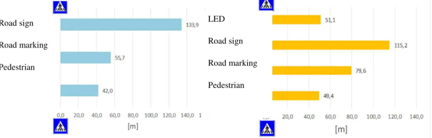
Figure 26. Pedestrian crossing element perception distance (Left OFF, Right LED) ... 63

Figure 27. a. The driver velocity profile in case of LED b. case of Control Situation ... 64

Figure 28 . Schematic view of dynamic driving task and different level of function ... 67

(13)

8

Figure 30 Test LAP: ACC ON and OFF events... 70

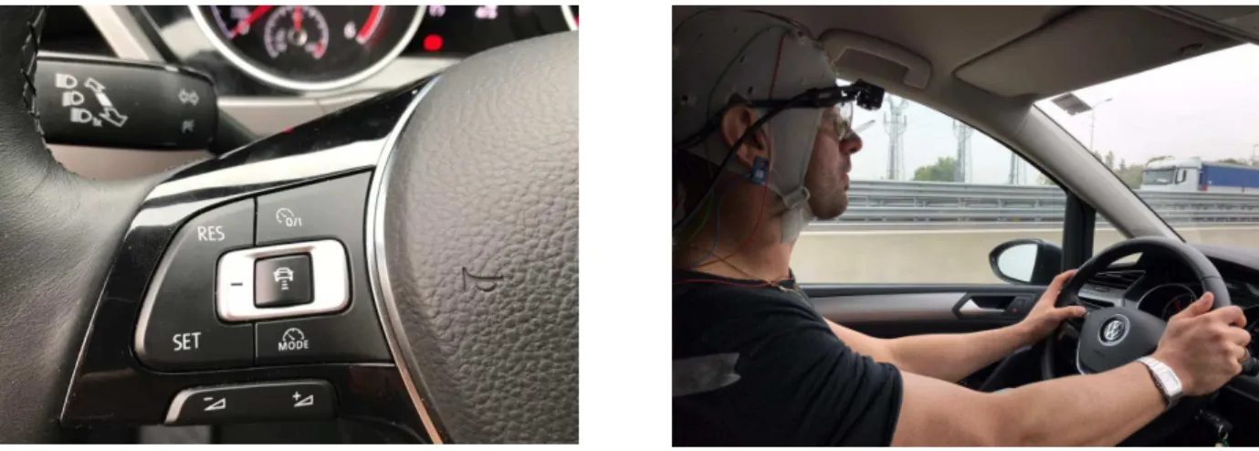
Figure 31 a. ACC system in the test vehicle ; b. EEG Helmet and ME during the test ... 71

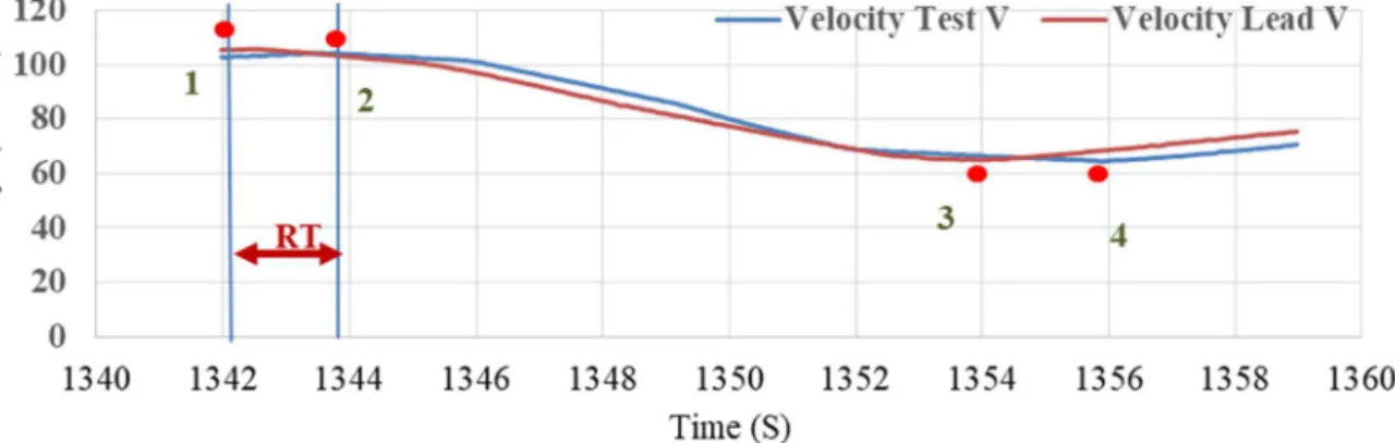
Figure 32.The velocity of test and lead vehicle vs Time –ACC OFF... 72

Figure 33.The velocity of test and lead vehicle vs Time –ACC ON ... 73

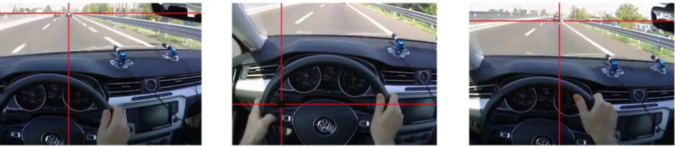
Figure 34. a. Driver gaze at the lead vehicle; b. driver gaze at dashboard; c. gaze back to lead vehicle ... 73

Figure 35. Driver attention and distraction percentage ACC ON and OFF ... 76

Figure 36 Braking reaction time during braking events-ACC OFF ... 76

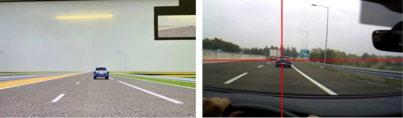
Figure 37 .a Driving simulator Virtual Environment; b. On- Road experiment Real Environment ... 80

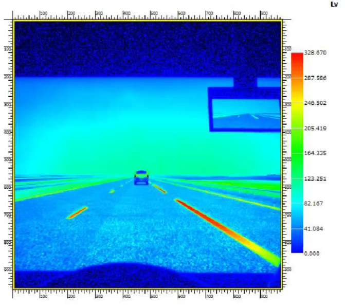
Figure 38. The luminance of the elements in the visual from 40 meters (cd/m) ... 81

Figure 39 . Adaptive Cruise Control activation switch ... 82

Figure 40 vehicle in front and braking light luminance from 40 meter (cd/m2) ... 82

Figure 41. Driving simulation Experiment Condition and Braking Events ... 83

Figure 42. a. Pupil core eye tracker, b. participant during the simulation with eye tracker ... 84

Figure 43. Eye-tracking calibration using 5 point ... 85

Figure 44 a. eye fixation segment; b. Excel file export of segment classification by software ... 86

Figure 45. Eye tracking Elements during the braking event ... 86

Figure 46. Driver Element distribution at an event with ACC OFF-MOTION ON ... 87

Figure 47. Driver Element distribution at event 2 with ACC ON_MOTION ON ... 88

Figure 48. Velocity profile of the test and lead vehicle- Event 1 ACC OFF ... 89

Figure 49. Velocity profile at event 1 during ACC on ... 90

Figure 50. Velocity during each event at condition with ACC OFF ... 91

Figure 51 Time to collision with ACC OFF ... 91

Figure 52. Reaction time with ACC OFF ... 92

Figure 53. Minimum Distance During Braking Event ACC OFF ... 93

Figure 54. Braking Distance with ACC OFF ... 93

Figure 55. Fixation Frame on attention element ACC On and OFF ... 94

Figure 56. Pupil diameter during the braking phases ... 95

Figure 57. Drivers visual attention during ACC OFF in real and simulator experiment ... 99

Figure 58. Drivers visual attention during ACC ON in real and simulator experiment ... 99

(14)

9

List of Tables:

Table 1 Vehicle Fixed Coordinate System ... 33

Table 2 Earth Fixed Coordinate System ... 33

Table 3 OBD available data from OBD II ... 49

Table 4. Driver performanc on-road experiment... 77

Table 5. Workload Index from EEG ... 77

Table 6. Self-evaluation workload index ... 78

Table 7. Eye-tracking gaze analysis ... 94

Table 8. T-test for the kinematic parameters ... 96

Table 9.Average and standard deviation of kinematic parameters during ACC OFF and ON ... 96

Table 10.Car following ACC OFF driver performance ... 97

(15)

(16)

11

List of Publications

This doctoral dissertation consists of the following publications that are referred to in the text by the case-study, all the papers are

Case Study I. N. Ghasemi “Investigating driver response to vehicle gear shifting system in motion

cueing driving simulator”, (Unpublished)

Case Study II. N. Ghasemi, H. Imine, A. Simone, C. Lantieri, V. Vignali, K. Finamore, “Longitudinal Motion Cueing Effects on Driver Behaviour: A Driving Simulator Study ”, Advances in Transportation Studies, Volume XLIX, Pages 91-102

Case Study III. N. Ghasemi, H. Imine, C. Lantieri, A. Simone, V. Vignali, E. Acerra “Innovative

technologies measurements to integrate Human Factor in Road Safety Review”, at International

Congress on Transport Infrastructure and Systems in a changing world, TIS ROMA 2019, Roma, Case Study IV. V. Vignali, M. Pazzini, N. Ghasemi, C. Lantieri, A. Simone, G. Dondi, “ The safety

and conspicuity of a pedestrian crossing at roundabouts: the effect of median refuge island and zebra

markings”, Transportation Part F Journal, Transportation Part F: Traffic Psychology and Behaviour,

Volume 68, Pages 94-104

Case Study V. M. Costa, C. Lantieri, V. Vignali, N. Ghasemi, A. Simone, “Evaluation of an

Integrated Lighting-Warning System on Motorists’ Yielding at Unsignalized Crosswalks During

Nighttime” Transportation Part F: Traffic Psychology and Behaviour, Volume 68, Pages 132-143

Case Study VI. N. Ghasemi, “Driver yielding behaviour at priority cyclist crossing using surrogate

measures”,(In progress)

Case Study VII. E.M. Acerra, M. Pazzini1, N. Ghasemi, V. Vignali1, C. Lantieri, A. Simone, G. Di Flumeri, P. Aricò, G. Borghini, N. Sciaraffa, P. Lanzi and F. Babiloni, “ EEG-based mental workload

and Perception-Reaction Time of the drivers while using Adaptive Cruise Control ”, 3rd International

Symposium on Human Mental Workload: Models and Applications, Roma, Italy

Case Study VIII. E. M. Acerra, N. Ghasemi, C. Lantieri1, A. Simone, V. Vignali1, F. Balzaretti, “

Perception-Reaction times of the drivers during the use of Adaptive Cruise Control ”, 28th annual

(17)

(18)

13

List of abbreviations and symbols

AADT Annual Average Traffic

ADAS Advanced Driving Assistant Systems

ACC Adaptive Cruise Control

BA Behavioural adaptation

DOF Degree of Freedom

DDT Dynamic Driving Task

EEG Electroencephalography

ET Eye Tracking

FFT Fast Fourier Transform

IAF Individual Alpha Frequency

MCA Motion Cueing Algorithm

PET Post Encroachment Time

PRT Perception Reaction Time

TTC Time to collision

(19)

(20)

15

Abst

ract

The present doctoral thesis discusses the ways to improve the performance of driving simulator, provide objective measures for the road safety evaluation methodology based on driver’s behavior and response and investigates the drivers’s adaptation to the driving assistant systems.

The related research activities were carried out in collaboration with the University of Bologna, Paris-Est University and Gustave Eifel university (IFSTTAR) in the form of a cotutelle PhD. The activities are divided into two macro areas; the driving simulation studies conducted in Gustave Eifel University (IFSTTAR) and on-road experiments organized by the University of Bologna.

The first part of the research is focused on improving the physical fidelity of the two DOF driving simulator with particular attention to motion cueing and vehicle dynamics model. The vehicle dynamics model has been developed in MATLAB-Simulink and has the ability of real-time calculation of the vehicle states and control the motion platform. During this phase of the research, motion cueing algorithms were developed to control the simulator movements and the effect of the motion cues on drivers’ behaviour was analysed through experimentation. The results of these studies are discussed in the case study I and II.

In the second part of the research, the driver performance and visual behaviour were studied on the road under different scenarios. The driver visual behaviour was recorded with the use of a head-mounted eye-tracking device, while the vehicle trajectory was registered with an instrumented vehicle equipped with Global Positioning System (GPS). During this phase, several case studies were developed to monitor drivers’ behaviour in the naturalistic environment. Case study III aims to integrate the traditional road safety auditing with an innovative driver behaviour monitoring system. The real road experiment with drivers was carried out in an urban arterial road in order to evaluate the proposed approach through innovative driver monitoring techniques. These same driving monitoring instruments were used for evaluating the improvement of a pedestrian crossing at the roundabout in case study IV. The eye-tracking data were evaluated in both studies in order to identify a driver visual attention indicator based on the participants gaze position and duration.

Significant attention is given to the safety of vulnerable drivers in urban areas during the naturalistic driving behaviour study. Case study V analyzed the driver yielding behaviour in approach phase to a bicycle priority crossing with the use of surrogate safety measures. The drivers’ performance

(21)

16 measures such as perception reaction time and gaze behaviour were used to assess the safety level of the crossing equipped with standard and innovative signalling systems. The improvement on the driver’s yielding behaviour towards an un-signalized crossing during nighttime and their reaction to an integrated lighting-warning system was evaluated in the case study VI.

The last phase of the thesis is dedicated to the study of Adaptive Cruise Control (ACC) with on-road and simulator experimentation. The on-road experimentation investigated the driver assistant system influence on the drivers' adaptation with objective and subjective assessment, in which an eye-tracking instrument and EEG helmet were used to monitor the drivers on a highway. The results are presented in Case studies VII and VIII and drivers’ visual attention was reduced due to adaptation to the ACC in the car following scenario. The results of the on-road test were later used to reproduce to the same scenario in the driving simulator and the adaptation of drivers’ behaviour with the use of ACC was confirmed through experimentation.

(22)

17

CHAPTER I

INTRODUCTION

(23)

18 Road safety engineering is a set of measures that aim to ensure safety on road networks, with the final goal of reducing the number of road accidents and injuries. These measures address the implementation of integrated actions considering all the components of the road network environment, driver, and vehicle.

According to the 2018 global status on road safety, road traffic injuries are the leading cause of death of children and young adults with the total fatality of more than 1.35 million around the world and about 50 million people seriously injured (World Health Organization, 2018). Accidents have a major impact also on the economy as a recent study of the word bank group shows that by reducing the road crash by half, the long term Gross Domestic Product (GDP) could increase up to 22% in some countries (Bose, et al.,2018).

Considerable steps have been made towards reducing the road fatalities, mainly with the implementation of safety systems in the vehicles (i.e. airbag, seatbelts), However, human errors are the main reason in occurring accidents. Studies on the crash causation by showed that in more than 94% of the crashes, the main accident contributor was the driver, from which 41% identified to have recognition error, 33 % decision error and 11% was the performance error (NHTSA, 2015).

Road safety analyses consider the concept of the driving task including control, guidance and navigation. The complexity of the information process increases from basic control to navigation task, whereas the safety impact of each level decreases from navigation to control. The driver controls the vehicle base on the visual sensory input from the road environment and the vehicle feedback. These skills are mainly learned by experience and executed automatically by the driver. The guidance and navigation skills, However, requires cognitive activity and the use of long-term memory. The first step to analyze the driving behaviour is to consider the physiological and mental capabilities of the driver such as visual field, reaction time, memory, task prioritization and anticipation. According to these models, the errors can be classified into different groups. The resource overflow error which is due to fatigue, stress and loss of vigilance may cause from the saturation of information. The failure of execution of the task might also occur due to poor coordination of task, poor perception of distance or misunderstanding of the road infrastructure. The error as a fault in the reasoning step is usually induced from an unexpected event, which the driver had not experienced before.

(24)

19 The road safety engineer is responsible for applying specific measures on the road environment component during the design, maintenance and during the daily operation of the road infrastructure. For example, in order to allow safe traffic operation, road infrastructure should provide adequate quality (visibility, self-explaining, durable pavement, protection) and must be consistent over space (consistency of the road elements and signaling with the environment) and should be also consistent overtime for the drivers (i.e. visual information adapting to operating velocity). Therefore there is a need for a procedure to measure the safety of the road since there is a significant gap between objective and subjective safety perceived level of risk from the road users. This problem is addressed in chapter 3, by introducing a methodology to integrating the driver behaviour (visual and velocity) with the existing road safety assessment methods.

The road infrastructure management approach is the systematic procedure for the examination of a road project or an existing road by a qualified technical expert (auditor), independent of the designer and the administrators. The increase in accident rate or accident severity is one of the main indicators. These guidelines define criteria and to carry out regular audits on the road, inspections on the existent infrastructures, implementation of the project and classify the roadways. Moreover, these guidelines have the main goal to direct, coordinate activities involved in the safety process.

The standard method for road infrastructure safety management starts with the ranking of the road sections, based on accident statistics and crash records. The analysis of road safety is a set of checklists on projects and inspections on existent infrastructures. The final aim is to identify sites which could potentially carry to accidents, verify the new infrastructure's safety or adjust existing roads, targeting investments to the road sections with the highest accident rate or highest accident reduction potential. Regular audits are not independent ones concerning the other, and they are part of a cycle where activities are consequential and iterative aimed to obtain safety improvement through optimized management of the road infrastructure. The complete cycle of activities by grouping all activities in macro activities is shown in Figure 1:

(25)

20 The Road Safety Review is an analysis of the current state of the road infrastructure by identifying the sections with highest accident rate and critical issues in order to plan the type of intervention for improving the safety level of the infrastructure. Considering the Italian legislation, the operating to assess of the Road Safety Review is composed of four steps (D.Lgs 35): network analysis, inspections, classification and intervention. The network analysis consists of the state of the motorway, road type, traffic data and accident analysis. This will be followed by an examination of the geometrical and functional structure of the road. The inspection program consists of the programming and assigning the expert for the realisation of the examination. During this phase, several parameters of the infrastructure will be investigated depending on the stage of the project. Among investigated parameters is visibility condition of the road, approach sight distance, junctions location, number of lanes, meteorological conditions, operating velocity, horizontal and vertical signs, road signing, roadside barrier condition, emergency parings, etc. (Ghasemi et al. 2019).

1.1. Measuring road safety with surrogate events

The standard method for road infrastructure safety management is based on the accident statistics and crash records. This method has some drawbacks, such as under-reporting accidents, lack of details in the police report and more importantly, it requires long observation periods. Estimating safety is one of the greatest challenges faced by those involved in safety research and management. It still is not possible to confidently attribute a resulting safety improvement to any implemented countermeasure because of the fundamental difficulty in measuring the countermeasures. Surrogate safety measures are new method designed to study road safety based on identification and examination of near miss events that with the growing use of intelligent systems in the vehicles, can be easily implemented to estimate the risk of road infrastructure.

The fundamental idea of the Traffic Conflict Theory (TCT) is that near-miss events can be used to investigate road safety instead of accidents. This TCT potentially will reduce the time of observation for assessing road safety and use objective measures such as operative velocity, distance and other time-based Surrogate measures for quantifying the riskiness of the event. The word conflict defined as when two or more road users approach each other in a way that a collision is about to happen if their movements remain unchanged. In order to investigate the surrogate event, usually, the events are being recorded and then analysed later using post hoc video analysis. The conflicts can be recorded stationary or in-vehicle by using video-based observation, semi-automated or fully

(26)

21 automated video analysis (Laureshyn 2010). The technological development made these data more accessible than before with a relatively low cost. The surrogate safety measures are also being used in driving simulator studies, in a controlled and safe environment that can provide robust data. Vulnerable road users such as pedestrians, cyclists suffer severe injuries more than protected road users (i.e. car, bus). The angle of the approach before the collision may have changed the patterns from head-on to rear-end. For collisions involving a protected road user, the point of impact influences the gravity of injuries. For example, head-on collisions are less dangerous than right-angle collisions. Collision at higher velocity produces more severe injuries than collisions at lower velocity due to a larger amount of kinetic energy released. There are indications that the relative velocity of the involved road users is a more important variable than the absolute velocity values.

Researchers obtained that the riskiness level changes in the reverse order to the frequency of traffic interactions. The concept as a pyramid of traffic event is that the pyramid is divided into several levels, each one representing the frequency of these events. According to this model, the higher the severity, the lower would be the frequency of the events. Therefore, dangerous and less frequent are accidents at the top of the pyramid (Figure 2).

A well known surrogate safety measure is the time to collision (TTC). The TTC is the expected time for two moving objects to crash if they remain at their present velocity and on the same collision course. The collision course is the necessary condition for calculating the TTC, and it can be used to evaluate the collision risk of various types of collisions. The minimum calculated TTC value used represents the riskiness of the event recorded during the entire event, rather than the value recorded at the time of evasive action. The lower TTC value corresponds to a higher conflict severity.

(27)

22 Post Encroachment Time (PET) is another surrogate conflict measure refers to the time lapse between the end of encroachment of passing the vehicle and the time that the through vehicle arrives at the potential point of collision (conflict zone). The main difference between PET and TTC is the absence of the collision course criterion. PET is easier to extract using a stationary camera as no relative velocity and distance data is needed.

1.2. Human factor in road safety

Human Factors was introduced as a technical term since 1930 with the growing use of man-machine systems in automation. The term human factor defined as the contribution of human to develop an error or failure in the machine function. As also mentioned before, the human factor plays a crucial role in road safety, since the critical reason for more than 90 % of road crashes in the motorways is driver recognition, decision, and performance error (Singh 2015).

The road design engineer should not only comply with the requisites of the vehicle (i.e. curve radius, stopping distance), but also should consider the driver behaviour towards the road infrastructure, and anticipate the reaction of different road users. Some of these are related to the traffic situation and maybe investigated using traffic analysis techniques; others are related to the human visual capacity, spatial perception and sense of orientation which are essential to detect obstacles, road sign and traffic lights.

The road transport system can be described with the model of the three key components: Driver (human), vehicle and the road environment (Figure 3). The study of the interactions between these components can be used to investigate the effect of each of these components on a traffic accident and to design assistant systems to increase road safety. A systematic approach to investigate the human-vehicle-environment should consider the human physiological and psychological capabilities and limitations in the design of road infrastructure and traffic management. These interactions can be listed as:

(28)

23 Figure 3. Driver-Vehicle- Environment system

• The interaction between vehicle and road environment: Described in several technical guidelines used by road engineer for designing slope, road radius, etc. which are mostly calculated based on the vehicle dynamic and road surface properties

• The interaction between driver and vehicles (man-machine interface). The ergonomic and response time of drivers and are taken into consideration by the car industry.

• The interaction between the driver and the road environment: This is the field of human factor specialists. These interactions are not well described in existing technical guidelines. However, they are crucial for driving; such as velocity, distance and depth estimation from the human sensory system

Road engineering standards should consider human behaviour, capabilities, and limitations since the design of the road environment affect the driver’s choice of velocity and position in the road significantly. For example, the reduction on the road width found useful to reallocate drivers towards the centre of the road, which gives them a recovery area for steering errors (Mecheri et al, 2017). The curb extension in the crosswalk could decrease the driver’s velocity and increases pedestrian visibility (Bella et al., 2015). The decrease in the visual contrast in the fog condition can reduce the ability of the drivers to estimate velocity and drivers underestimate their speed (Pretto et al., 2008) (Caro et al., 2009).

Drivers actively search for information to adapt their behaviour (velocity, position) according to the road characteristics and perceived signals. During a trip, drivers should be able to quickly recognize the main function of the travelling road and signals. The correct application of the road signs and road markings ensures road safety and affect the situational awareness of road users. Road marking characterises by properties such as retro-reflection, colour, skid resistance and durability A recent

(29)

24 study in Switzerland, where the yellow marking was used at the zebra crossings, illustrated that the use of glass beads material in road marking can improve the retro-reflectivity of the zebra crossing at night (Burghardt et al. 2019). The colour of the road markings and the retro-reflectivity of the pavement materials also can improve the conspicuity level of the vulnerable user (Costa et al., 2018). Additional lighting features can be used at night such as flashing LED curb and found useful to reduce the velocity of the drivers (Bella et al., 2015) (Samuel et al., 2013).

The workload level of the driver might influence their performance. The workload is a multidimensional phenomenon and can affect the driver in many ways. Having a low amount of information or overload of information both may lead to significant errors. Information underload decreases the driver’s attention and awareness that may lead to increasing velocity. On the contrary, high workload leads to perception error or reaction delay. Various measures are being used to study the workload such as driver's eye glancing patterns, Number of glances, duration and the location of glances made while performing a driving task or directly by measuring the activity of the brain using the electroencephalographic technique (EEG).

1.3. Driving simulator and road safety

Driving simulation development started in the 60s using analogue computers and electronic circuits. In 1965, the American Society of Mechanical Engineers published a report outlining the development of a driving simulator in which drivers were seated in a stationary vehicle cab in front of a projection system re-playing colour video recorded from a real-world scene (Fisher et al., 2011). Driving simulators can vary from very simple simulators using a joystick or keyboard control with a primary road environment displayed on a PC screen to multi-million-dollar Simulators with full-size vehicle cabin and motion restitution, 6 degrees of freedom and a 360° field of view.

Driving simulators are powerful tools which allow testing complex tasks at a relatively low cost. They are useful to study driving behaviour and represent an efficient alternative to test track evaluations. Repeatability of experimental conditions, safety and cost-effectiveness of the tests are some of the motivating factors for using driving simulators. Driving simulators make it easy to test and compare different existing or new road configurations or equipment. Thus, they are powerful tools to investigate driving behaviour, allowing them to determine how road design perceived and understood by the drivers and how they may respond to them.

(30)

25 Experimenting high-risk scenario in the virtual environment is the main advantages of driving simulators. They provide total control over the simulated events in a safe environment. It is possible to present the participants with driving tasks that would be challenging to study on a test track or the road, either because they are dangerous, or they rarely occur. For instance, driving simulators can be used to study populations at risks such as elderly pedestrians or scenarios with traffic congestion. They can also be used to investigate the driver’s fatigue, impairment and medical issue. The driving situations can be reproduced as many times as needed, and this facilitates behaviour comparisons of several participants in the same scenario. Driver feedback to the virtual environment and driving performance measures such as steering wheel, pedals, gear change can be recorded using high-frequency sensors.

When it comes to a driving simulator, the advantages are related to the possibility of bypassing road tests with real vehicles. However, the fidelity of the simulator must be ensured, so that results in the driving simulator are comparable with those obtained with a real vehicle. In other words, the driving simulator needs to be validated. This is a very important step for generating meaningful test and the credibility of the simulator experiments for road safety studies. This validity can be investigated by comparing the behaviour of the drivers in the simulator (behavioural validity) by comparing with a similar scenario in another simulator or a real road experiment (relative validity). Another validation method could be done by comparing the physical variable (i.e. velocity) in a real and simulated environment. Statistical methods such as analyse of variance (ANOVA) or correlation analysis must be used to find the statistical significance between the simulated and real road test results. In the last chapter of the thesis, some of these aspects were discussed using surrogate safety measures.

1.4. Thesis Contribution

This thesis advances the state of the art in the human-vehicle-road interaction and proposes design solutions for enhancing road safety based on the drivers’ performance and objective measures. The main focus being on the drivers’ braking and yielding behaviour and the thesis aimed to enhance the understanding of the drivers’ performance through various designs and stimuli on road and followed up by simulation. Another major contribution of this thesis is the experimental work on the motion cueing platform and the impact on human depth/distance perception in the virtual environment.

(31)

26 The drivers' adaptation to the automation solutions is another topic covered by this thesis, in particular for the car following/braking scenario with the use of Adaptive Cruise Control (ACC). An original approach for estimating the human visual distraction was used in the thesis and the proposed methodology was applied to the real road and simulation experimentation.

1.5. Thesis outline

The thesis is structured in five chapters and eight case studies at the end. Chapter 1 is an introduction to the thesis. chapter two is focused on the vehicle dynamic model and the motion cueing platform and presents two original case study on the motion perception of drivers in the simulator. In chapter 3, Innovative road safety measures and the advanced monitoring technologies for road safety audit is presented with two case studies. In chapter 4, the surrogate safety measures were used to compare design solutions at pedestrian and bicycle crossing with two case studies And n Chapter 5, the driver adaption to ACC in a car following scenario was investigated, using a microscopic traffic simulator and on-road investigation with two case studies.

(32)

27

CHAPTER II

VEHICLE DYNAMICS AND 2DOF MOTION

PLATFORM IMPROVEMENT IN THE

(33)

28 Driving dynamic task (DDT) is defined as all the real-time operations and tactical functions required for operating a vehicle on the road, excluding the selection of itinerates and trip scheduling that are strategic. The operations such as lateral vehicle motion control via steering wheel (operational), Longitudinal vehicle motion control with pedals (operational), Monitoring the driving environment (via object and event detection), recognition, classification, and response preparation (operational and tactical), object and event response execution (operational and tactical), Manoeuvre planning (tactical), enhancing conspicuity via lighting and signalling (tactical) are all considered as the dynamic driving task (SAE J3063, 2015).

Vehicle dynamic model (VDM) is in charge of simulating in real-time the entire vehicle states that during dynamic driving task are necessary for the driver. This information later is being displayed on the dashboard (i.e. velocity, rpm), through a Human-machine-Interface (HMI) or use as input for visual, sound or motion cueing systems. The vehicle dynamic model depends on vehicle characteristics such as the engine, braking system, gear shifting system, suspension and even driving assistant system or cabin control. This makes driving simulator an important research tool for vehicle manufacturing companies to test their vehicle design and provide useful information for improving the design of the road infrastructure.

The visual cue is the primary source of information for monitoring and event detection; however, the motion and proprioceptive feedback of the vehicle to the input signal is giving information to the driver to adapt his control input according to the vehicle performance. The movement of the simulator can enhance the driver perception in the virtual environment with the correct motion according to the visual stimuli. However, reproducing the full-scale accelerations of the real vehicle is very costly if not impossible, and therefore, motion cueing algorithms should be used to reproduce the motion in driving simulators. The motion cueing algorithm uses the vehicle states (in real-time) from the vehicle dynamic model and performs calculation considering human vestibular perceptual limitations. This chapter first explains the simulator architecture and the vehicle dynamic model used for the simulation. Different gear shifting systems were implemented to investigate driver behaviour. Finally, experimentation involving participants conducted to test the simulator motion in different sessions. All the activities in this chapter are case-study I that you can find in the annexe.

(34)

29

2.1. Simulator architecture

The choices of the structure and motion bases for the SIMU-LACET driving simulator are motivated by the necessity to produce sufficient perception while driving as well as by financial design constraints. Thus, the objective of the simulator project is not to reproduce all of a real vehicle’s motions, but only the longitudinal movements or surge, and yaw, which makes this a 2DOF driving simulator.

The component of the simulator and connections between them is illustrated in Figure 4. The acquisition system is composed of an industrial microcontroller and has both analogic and digital input/output. This allows the control of the actuators in the desired position, velocity or torque (used for the steering wheel force feedback). A bidirectional information exchange protocol is defined between this electronic board (I/O) and the PCs dedicated to dynamic simulation and traffic simulation. The communication is performed through CAN port between the electronic board and the XPC target.

1. XPC Target: This PC is connected through a CAN interface directly to the I/O board. This board communicates to the MATLAB PC and the actuators. It is also linked through an Ethernet connection to the Traffic model PC.

2. MATLAB-Simulink PC: The Simulink interface is installed on this PC with the vehicle model and the real-time simulations are being controlled from this PC.

3.

(35)

30 4. Sound cueing PC: The sound cues such as road-noise, engine, other traffic during the simulation is simulated using this PC which consists of software managing the sound effects during the simulation. It works with a sound card mounted under the platform, while the speakers which are mounted in the motion cabin reproduce the sounds;

5. Traffic Model PC (Dr2): This computer simulates the road environment, traffic and the driving scenario. The software ArchiSim2 is used for the programming of the traffic and allows different time, distance or velocity criteria to be used for the simulation of the events. 6. Visual Rendering Unit: Three Computers are connected directly with PC Dr2 and broadcasts The pictures on three fixed screens visual cueing mounted on the cabin. The screens are 4K resolution and 100 Hz frequency (Figure 5) providing 180° of horizontal and 36° of vertical Field of view (FOV).

2.3. Vehicle dynamic model (Matlab-Simulink)

The vehicle dynamics model, responsible for calculating the response of the vehicle based on the driver control input, is implemented on MATLAB-Simulink software and can be modified and controlled with the same interface software. The Vehicle Dynamic Model shows the relations between the different parts of the vehicle model in a graphical format. In this way, the various inputs can be traced graphically and the relations between the inputs are in MATLAB script format. Each of the different models has sub-layers to make the simulation work and to show the relative outputs of the different parts of the model. As mentioned before, this model should represent vehicle motions and control feel conditions in response to driver control actions, road surface friction conditions and aerodynamic disturbances. All required vehicle feedback is computed in real-time for commanding the visual, motion and sound simulation systems. In addition to the vehicle model, the motion cueing algorithms and the commands to the actuators are also controlled and can be adjust/modified in the MATLAB-Simulink model.

(36)

31 The proposed dynamic vehicle model is nonlinear. The vehicle model allows the determination of the virtual vehicle states according to the driver’s control input. The vehicle dynamic model concerns the computation of the dynamics and the kinematics as a function of the driver input and the road characteristics. The model contains as main inputs the commands (Throttle, Clutch, Brake, Gear.) which influence the longitudinal control of the vehicle and the steering as the lateral control input. The kinematic elements can greatly influence the vehicle dynamic behaviour. This is due to the existing interconnection between different parts of the vehicle. Due to the complexity of a complete vehicle, the model is limited to four interconnected subsystems: the chassis, the suspensions, the wheels and their interaction with the ground. The vehicle characteristics used in this simulator belong to the Peugeot 406. The engine is simulated using the real engine dataset from the Peugeot 406 engine characteristics (engine torque curves, clutch pedal position, accelerating proportioning, etc.). After updating the vehicle’s state, the relevant resulting information is sent to the cabin’s dashboard and to the traffic model server. The platform is equipped with several sensors and electric board in order to have information feedback on the control system states. The vehicle model based on the Peugeot 406 and is implemented in the MATLAB-Simulink. The model after compiling computes the states of the vehicle with the frequency of 1000 Hz. The output of the vehicle model is necessary to send the location of the vehicle to the virtual environment (visual) and the longitudinal acceleration and yaw rate are also necessary to reproduce the cabin motion.

In this model, the vehicle is considered as one body with 6DOF (surge, sway, heave, roll, pitch and yaw). The engine part is modelled by a combined mechanical and behavioural approach based on the vehicle’s general characteristics (engine torque curves, clutch pedal position, throttle, etc.). Each of the blocks in the Simulink model is for modelling a different part of the vehicle dynamics as shown in Figure 6.

(37)

32 The modelling of all the processes that take place inside an internal combustion engine is very complex and it requires many parameters which are not easy to obtain. Moreover, the objective of the research does not require high precision in that direction. The choice is to use the cartography of the engine given by the constructor. This kind of 3-D table requires at the input, the acceleration rate and the rotational velocity of the motor and provide at its output, the engine torque.

The engine model needs to consider the clutch, braking torque, gear transmission and throttle position. The clutch and throttle model are shown in figure 7. Two thresholds are set on the clutch pedal rate. These two values have been defined directly on the simulator. The rate of pressure is measured in percentage, where 100% corresponds to the clutch fully pressed. Between the two threshold values, a linear relationship between the percentage of pressure and the transmitted torque is supposed.

Figure 7. Vehicle Model Blocks

2.3.1 Vehicle Trajectory calculation

The vehicle motions are defined concerning a right-hand coordinate system (fixed with the vehicle) which originates at the centre of gravity and travels along with the vehicle. Vehicle motion is described by the velocities (forward, lateral, vertical, roll, pitch and yaw) concerning the vehicle fixed coordinate system, where the velocities are referenced to the earth fixed coordinate system (Figure 8).

(38)

33 Vehicle attitude and trajectory tough the course of manoeuvre are defined concerning a right-hand orthogonal axis system fixed on earth which is usually selected in the way that coincides with the vehicle fixed the coordinate system at the point where the manoeuvre is started.

Table 1 Vehicle Fixed Coordinate System

Table 2 Earth Fixed Coordinate System Earth Fixed Coordinates (R0) Definition

X Forward travel

Y Travel to the right

Z Vertical travel (+ downward)

ψ Heading angle (angle between x and X in the ground plane)

ν Course angle (angle between the vehicle’s velocity and X-axis)

β Sideslip angle (angle between x-axis and vehicle’s velocity

vector)

The relationship of the vehicle fixed coordinate system and the earth fixed coordinate system is defined by Euler angles. Euler angles are given by a sequence of three angular rotations. Beginning

Vehicle Fixed Coordinates (RC) Definition

x Forward and on the longitudinal vehicle plane of the symmetry

y Lateral out the right side of the vehicle

z Downward with respect to the vehicle

P ( ) Roll velocity about the x-axis

q ( ) Pitch velocity about the y-axis

r ( ) Yaw velocity about the z-axis

(39)

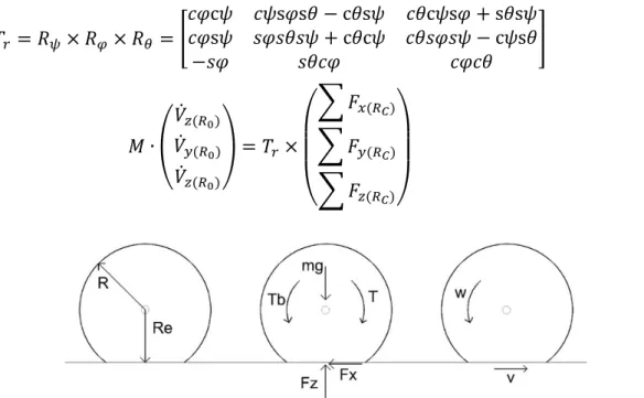
34 at the earth fixed system the axis system rotates around the yaw (z-axis), then in pitch (y-axis) and then in pitch (x-axis). In order to transform the fixed coordinate system “R0 to the centre of gravity coordinate system “Rc”, a transformation matrix must be constructed “Tr”.

= × × = cs s s − c s+ c c c s + s s− c s − (3-1) ∙ !( )( ) ( ) " = × # $ $ %& '(( )) & '!( )) & '( ))* + + , _(3-2)

Considering a simplified motion dynamics of a quarter vehicle, the longitudinal dynamics may get calculated for braking and acceleration phase using the effective rolling radius (Re) assumed the same for all the wheels (Figure 9). The single-wheel braking model is composed of a single wheel of radius R which moves longitudinally with a contact velocity of “ν” and angular velocity of “ω”. The longitudinal force “Fx”, is calculated from the vertical reaction force ”Fz” which balances the weight on the wheel, The breaking torque “Tb” and the traction torque “T” from the motor. Applying Newton’s law to the wheel dynamic model gives us the following equations of the motion for the quarter vehicle, Where “Jw” and “Re” are the inertia and effective rolling radius of the wheel respectively:

-./( = '/( (3-3)

012/ = ( /− 3/) − '/(∙ 4 (3-4)

'/5− -/. 7 = 0 (3-5)

(40)

35

2.3.2 Vehicle Longitudinal sliding model:

The generation of the forces in the wheel road model is always leads to some sliding in part of the contact zone between the wheel and the road surface. A longitudinal tractive force produces at wheel/road contact point when the tractive torque is applied on the wheel and respectively a longitudinal braking force may apply by applying the braking torque on the wheel. This relative motion determines the wheel slip properties, which in longitudinal motion can be characterized by:

9(= : =2/(∙_;4− ;/(

/( => (;/( > 2/(∙ 4) Braking

9( = : =;/(− 2_; /(∙ 4

/( => (;/( < 2/(∙ 4) Accelerating

(3-6)

The longitudinal slip “κ” is negative in case of braking and positive in case of traction. “ κ=0”, implies the steady-state free roll situation and if it reaches “ κ=1” means that the wheel is completely locked. Very large values of “ κ” may happen when driving on very slippery roads. Lateral slip is also defined as the ratio of the lateral velocity to forward velocity of the wheel. Where “α” is the lateral slip angle for each wheel and the νiy and νix are wheel lateral and forward velocities.

9! = tan(L/) = −;_;/! /(

(3-7) To take into account the combined slip condition, when of the braking (or accelerating) slip effects integrate with the lateral slip, some modifications are needed in the tyre model. This is done using the elliptic approximation; the wheel slip ratio is as follow:

9 = M9(N+ 9!N (3-8)

Several types of research developed to describe the tire behaviour with two main approaches; physical and empirical models. Physical models are more complex and use finite element methods (FEM) which are time-consuming and are not suitable for real-time simulation. In this model, the Burckhardt model is being used with the dry condition, with the possibility of changing the pavement condition. Burckhardt method is based on a set of factors, which vary according to the type of the road surface type. The friction or adhesion coefficient is defined as the ratio of the frictional forces acting on the wheel plane depending on the normal wheel force:

'(9) = ' ∙ O(9) = ' ∙ (PQ∙ (1 − STUV∙W) − PX∙ 9) ∙ STUY∙W∙Z∙ (1 − P['N) (3-9)

(41)

36 C1: the maximal value of the friction curve: C1=1.28

C2: corresponds to the shape of the friction curve: C2=23.99

C3: the difference between the maximal value of the friction and 1. : C3= 0.52 C4: depends on the maximal velocity of the wheel. : C4=0

C5: represents the influence of the vertical load on the wheel. C5=0

2.3.3. Vehicle lateral sliding model

The steering wheel block computes the angle of the front wheel based on the commands from the cabin. To have a realistic simulation, the steering angle and the wheel angle from a real vehicle was estimated as follows:

δ], = (Steering Angle/10) (3-10)

In order to calculate the side slip angle, the single-track model (bicycle model) is developed in order to find the geometrical variables of the lateral dynamics model (Figure 10). Using this simplified model, only a single tire sideslip angle is calculated for the left and the right wheels, given as:

L_] = a − ( !+ b ( ) (3-11) L = −(cde cf ) (3-12) -(. − ;. b) = '(g+ '( + '(4 -(; + .. b) = '!g∙ cos a + '! + '(g ∙ sin a (3-13) 0 ∙ b = iQ∙ '!g∙ cos a − iN∙ '! + 4+ iQ∙ '(g∙ sin a

(42)

37 The equations of the motion are based the single-track model in planar motion. Where r is the yaw rate, u and v are longitudinal and lateral velocity in Rc frame. The equilibrium must hold in lateral, longitudinal and yaw direction with the force of the tires and the moment acting on the vehicle

2.4. Motion cueing platform:

The motion cueing platform is composed of two separate structures and drives. The longitudinal rail is located on the top of the rotating circular platform. The longitudinal upper structure can move linearly along the rail. A pulley-belts system is being used to move the cabin powering from a brushless servo motor (SMB 80). The lower structure provides yaw angle cabin rotation by using a circular platform in which the servomotor directly rotates the upper structure with wheel support in the front of the cabin. The vehicle motion simulation structure is shown in Figure 12. The participant in the driving Simulator cabin gives control input from the steering wheels and pedals to the vehicle dynamics model which generating the vehicle states. These states then will be used to mock the desired motion cues on the platform using the motion cueing algorithm. Two actuators generate the motion in the two degrees of freedom space of the cabin (yaw and longitudinal) using the desired platform states.

Motion cueing algorithms (MCA) render the physical motion of the simulated vehicle in real-time to provide a multi-sensory environment for the driver (Figure 11). The MCA goal is to: Keep the motion platform within the physical boundaries, stimulating the motion cue within the driver perception threshold and return the platform to its neutral position

(43)

38

2.4.1. Motion cueing algorithm

The classical algorithm was the first motion cueing algorithm for simulators, initially used in the 6DOF flight simulators at NASA Ames Research Centre. The first motion cueing algorithm only rendered the high-frequency domain, whereas the second version introduced the cueing of the low-frequency domain through the tilt-coordination. Nonetheless, the physical limitations of these first hexapods were considerable, and because of that the maximal displacement was very poor and since all the motion had to be cued, the parametrization of the algorithm was highly conservative and made considering the worst-case scenario, penalizing the rest of motion cueing. Nowadays, technological progress and advance knowledge of this algorithm overcame these problems.

A non-linear scale factor was introduced and implemented for both surge and yaw motion The non-linear scale factor is then obtained as:

j'/(=klmn(, j'm/o, p/) = S(T(∗nr) (3-14)

Where _=kl_mn(= Maximum input;_j'_m/o = Minimum scale factor;,_p_/ = Input Acceleration;, x = Scale parameter and the scaled input j skl is, where, p_/ = Acceleration input at i-time and j'_/ = Scale factor calculated for the input p_/.

j skl = j'/ ∗ p/ (3-15)

(44)

39 In this way, fixing the maximal acceleration and the minimal scale factor to be applied to this acceleration, the procedure generates each time a new non-linear exponential equation to calculate the scale factor to be used for each input.

For calculating the longitudinal acceleration input, considering_p _mn( _{= 0.8 7, being O}_mn( in the dynamic model 0.8; j'_m/o = 0.5. As a result, the exponential form to calculate the scale factor is:

j'/ = S(Tu.uvvX∗nr) (3-16)

And for the yaw motion input, with the absolute maximum yaw rate for the limit case of ISO chicane at 100 km/h is 22.11 o_{/s, and using SF}

min = 0.5 the scale factor is

j'/ = S(Tu.uXQX∗!w) (3-17)

The classical algorithm is developed by the combination of the washout and tilt coordination algorithm. The filters separate the frequencies of the linear acceleration for the displacements and rates for the rotations in high-frequency components and low-frequency components. It is by treating those that the classical algorithm cues a motion compatible with the limits of the platform. First, high-pass filter F1 passes the high-frequency components of the scaled signal. These components represent the transitory component of the signal, namely the variation of acceleration. A typical representation of the filter through the transfer function of a second-order problem is the following:

x = _N _{+ 2ξ}NyQ

Q2Q+ 2QN x . =kl.|

(3-18)

where:, k1 = Gain;, ω1 = Second-order system undamped natural frequency;ξ1 = Damping ratio.

Figure 13. Classical Motion Algorithm for Translational Motion

The first high pass filter F1 only collects the transitory acceleration; This signal is then double integrated for the acceleration of integrated once for the rate to obtain the position. A second high-pass filter F2 is then applied to this signal, which is called a washout filter. This filter allows the platform to bring back the cabin to its initial position after each transitory acceleration. It is by regulating the parameters of both filters which is possible to control the time needed to bring back

(45)

40 the platform to its initial position, the amplitude of the signal and therefore also the space used by the platform.

When adjusting the MCA, it is important to define the parameters so that the perceived accelerations are not inconsistent with the rest of the motion, the so-called false cues. These reduce the quality of immersion and create a degradation of simulated vehicle control. This incoherence in motion perception can be removed by regulating the filters. In general, it is possible to distinguish three principal sources of false cues:

• Post-filter acceleration exceedance:

After applying the high-pass filter to the simulated acceleration or rate, the filtered signal tends to follow the simulated signal in the transitory phase, whereas it vanishes when it comes to continuous accelerations. However, when the acceleration vanishes, an incoherent perception could be generated because of the motion conflicting with the rest of the simulation. Therefore, the overflow must be under the perceptive motion threshold of the vestibular system.

• Platform return to the neutral position

The washout filter purpose is to bring back the platform to its neutral position when continuous components of the input occur. However, the platform displacement to its neutral position might alter the perceptive coherence on the simulator. If the platform is moved in the opposite direction of the vehicle simulated motion with higher amplitude than the perceptive threshold of the vestibular system, a sensorial incoherence between visual perception and motion perception might occur;

• Sudden changes in input acceleration:

This is a case typical of the longitudinal motion. Generally, in this driving situation, protracted braking is generated. In the stopping manoeuvre, the acceleration goes from zero to a negative value, while the filter allows the driver only to perceive the transitory component. In the continuous acceleration phase, the acceleration remains negative, and the driver does not perceive any inertial effect. However, at the end of braking, the vehicle’s simulated acceleration is characterised by a relevant jerk, going from negative to positive. The virtual world of the simulation displays a vehicle perfectly still, while the platform cues a negative acceleration. This situation might be perceived as incoherent and creates unpleasant feelings in the driver.

(46)

41

2.5. Case- Study I

The vehicle modelling is a very important part of the driving simulation studies. The longitudinal and lateral sliding models, type of the surface, engine power and the assistant systems in the vehicle can change the driving simulator experience and driving performances.

The case study I aimed to describe in brief the vehicle modelling used in the simulator and focused in particular the effect of different gear change system on driving behaviour in the motion cueing simulator. The motivation of the experiment found after observing that drivers had difficulties to use the correct gear in the simulator. Therefore different gear shifting scenarios were developed in the simulator to see if the various gears shifting scenario would alter the motion perception of the participants. In addition to the manual gear shift, Sound gear shift assistant (Beep session) was developed. A beep sound is implemented to be activated when engine rpm was more than 4800. In this way, not only very high RPMs are avoided, but the driver was instructed to change the gear when changing the gear. The automatic gear change is implemented, that was automatically changing the gears so that the RPMs stay in the identified ideal range of 2000 > rpm > 4300.

The following scenarios were tested with 19 participants in the driving simulator with the driving task involving car following and braking, 2 chicanes and one overtaking manoeuvre.

1. Manual Session: in this session, the participant is free to adopt the gearing strategy 2. Assisted Session: in this session, the sound gear shift assistant is activated;

3. Automatic Session: in this session, the participant uses the automatic gear change

2.5.1. Discussion:

Drivers were adapting their behaviour with different gear shifting system in the simulator study. The result of the experiment did not show a significant difference by the repeated measure ANOVA significant test between the sessions for the studied indicator, namely maximum lateral, longitudinal acceleration or the RPM of the engine. The same adaptation might be seen when drivers using different vehicles in the real road, meaning that despite different performance and features of the vehicles, the drivers can control the vehicle in the road environment. The results are essential for the authors for the validation of the simulator performance and the 2DOF motion platform.

(47)

42

2.6. Case Study II:

This experiment focuses on the driver’s evaluation of the longitudinal motion in the car following scenario. The test features three sessions, and in each one of them, one of the MCA is implemented to reproduce the motion cues. The whole experiment lasts about 40 minutes, including 10 minutes of familiarization with the test. During the test scenario, the participant has to follow the lead vehicle in two lanes highway After 4 acceleration and 3 deceleration phases, the simulation ends when the subject reaches again the lead vehicle (as shown in figure 14).

Figure 14. Lead vehicle velocity profile

Three different algorithms, featuring three different transfer functions of the scaled acceleration, have been implemented for the longitudinal case. The algorithms structures are shown below. Each session on the driving simulator is evaluated concerning motion cueing by nineteen subjects employing two questionnaires. Both the questionnaires use a Likert scale, a psychometric scale usually involved when the rating is questionnaire-based. It aims to let the participants specify their level of agreement or disagreement on a usually symmetric agree-disagree scale for a series of statements, capturing the intensity of their feelings. By the strength of their agreement, it is possible to evaluate the sessions. Likert scale is also used featuring other characteristics, as in the first questionnaire. This one is the Simulator Sickness Questionnaire (SSQ) developed by Kennedy, featuring a four-points Likert scale to evaluate how much a symptom is affecting the participant after the session (R.S. Kennedy et al., 2003).

(48)

43

2. Motion Cueing Algorithm II: Fourth-order transfer function with non-linear Reymond

3. Motion Cueing Algorithm III: Third-order transfer function

2.6.1. Discussion:

The results of the case study II showed that longitudinal motion cues might affect the driver’s perception of the distance in the car following scenarios using independent T-test statistical test. The use of different motion cueing algorithm did not affect the driver’s performance in the driving simulator; however, the drivers were more satisfied with motion algorithm III and the Friedman statistical test confirmed the significance of the difference in the answers of the questionnaires. It is worth mentioning that the preference of the motion cueing in the simulator was different from the participants and might be affected by their expectations.

The result of the case study II was found very important for the choice of motion cueing algorithm and parameters in the simulator and showed the importance of motion cueing for the distance perception and immersion of the participants in the driving simulator study. The driver’s braking distance had a significant variation in the absence of the motion with comparison to the motion cueing sessions.

The reaction time of the drivers was investigated in the car following scenarios but no significant difference was found in the result. This is suggesting that the driver’s cognitive and motor skill was not influenced by the motion and therefore the simulator remains effective with different motion cueing condition to study the human performance measures in the man-machine interface system. The outcome of the case study II, motivated the author to study the driver visual behaviour in the simulator to investigate driver visual and performance in the car following scenario in the last chapte

(49)

(50)

45

Improvement of the driving simulator control and comparison between driver-road-vehicule interaction in real and simulated environment

HAL Id: tel-03033387

https://tel.archives-ouvertes.fr/tel-03033387

comparison between driver-road-vehicule interaction in

real and simulated environment

Navid Ghasemi

To cite this version:

in cotutela con Università Paris-Est

DOTTORATO DI RICERCA IN

Ingegneria Civile, Chimica, Ambientale e dei Materiali

Ciclo XXXII

IMPROVEMENT OF THE DRIVER SIMULATOR CONTROL AND

COMPARISON BETWEEN DRIVER-ROAD-VEHICLE INTERACTION IN

REAL AND SIMULATED ENVIRONMENT

Presentata da:

Navid Ghasemi

Coordinatore Dottorato

Supervisore

Supervisore

Co-Supervisore

Contents

List of Figures

List of Publications

List of abbreviations and symbols

Abst

ract

CHAPTER I

INTRODUCTION

1.1. Measuring road safety with surrogate events

1.2. Human factor in road safety

1.3. Driving simulator and road safety

1.4. Thesis Contribution

CHAPTER II

VEHICLE DYNAMICS AND 2DOF MOTION

PLATFORM IMPROVEMENT IN THE

2.1. Simulator architecture

2.3. Vehicle dynamic model (Matlab-Simulink)

2.3.1 Vehicle Trajectory calculation

2.3.2 Vehicle Longitudinal sliding model:

2.3.3. Vehicle lateral sliding model

2.4. Motion cueing platform:

2.4.1. Motion cueing algorithm

2.5. Case- Study I

2.5.1. Discussion:

2.6. Case Study II:

2.6.1. Discussion:

Chapter III

THE INTEGRATION OF HUMAN FACTOR IN

ROAD SAFETY USING INNOVATIVE