Evaluation of the effect of geometrical parameters on stope probability of failure in the open stoping method using numerical modeling
Shahriyar Heidarzadeh1, Ali Saeidi2, Alain Rouleau3 Correspondence
Shahriyar Heidarzadeh, Department of Applied Sciences, University of Quebec at Chicoutimi, Chicoutimi (Quebec) G7H 2B1, Canada, Tel : +1 (418) 545-5011 ext. 2589, Email : [email protected]
Present address
Department of Applied Sciences, University of Quebec at Chicoutimi, Chicoutimi (Quebec) G7H 2B1, Canada
Abstract
Stress-induced failure is among the most common causes of instability in Canadian deep underground mines. Open stoping is the most widely practiced underground excavation method in these mines, and creates large stopes which are subjected to stress-induced failure. The probability of failure (POF) depends on many factors, of which the geometry of an open stope is especially important. In this study, a methodology is proposed to assess the effect of stope geometrical parameters on the POF, using numerical modelling. Different ranges for each input parameter are defined according to previous surveys on open stope geometry in a number of Canadian underground mines. A Monte-Carlo simulation technique is combined with the finite difference code FLAC3D, to generate model realizations containing stopes with different geometrical features. The probability of failure (POF) for different categories of stope geometry, is calculated by considering two modes of failure; relaxation-related gravity driven (tensile) failure and rock
1 PhD Candidate in Geomechanics, Department of Applied Sciences, University of Quebec at Chicoutimi, Chicoutimi
(Quebec) G7H 2B1, Canada
2 Professor, Eng., Ph.D. Department of Applied Sciences, University of Quebec at Chicoutimi, Chicoutimi (Quebec)
G7H 2B1, Canada
mass brittle failure. The individual and interactive effects of stope geometrical parameters on the POF, are analyzed using a general multi-level factorial design. Finally, mathematical optimization techniques are employed to estimate the most stable stope conditions, by determining the optimal ranges for each stope’s geometrical parameter.
KEYWORDS: Stope stability, stope geometrical parameters, probability of failure, general
factorial design, numerical modeling, Sublevel open stoping.
1. Introduction
The stability of underground excavations has become a critical issue in the mining industry due to the growing trend of extracting deeper mineral resources. Open stoping underground excavation method is the most widely practiced technique in Canadian underground mines [1–4]. Open stoping creates large underground openings called “Stopes” whose level of stability must be assessed. Maintaining stope stability not only provides safety for the workforce and underground equipment, but also contributes to the mines production capacity and profitability by minimizing unplanned ore dilution [4–7].
Although the open stope stability state is significantly affected by external parameters such as the applied natural and mining-induced stresses, and the surrounding rock mass geomechanical characteristics [8–12], the stope geometry plays a key role in defining the level of stability [3] [12] [13].
Underground instability and the probable failure conditions, for open stopes located in deep hard rock, occur as a result of high magnitude mining-induced stresses [14]. Effects of open stope geometry (shape, size and inclination) on the state of stability, can be evaluated by using different analytical, empirical and numerical approaches. Numerical methods offer more advantages and less drawbacks compared to the other two methods [15], therefore they are widely used to analyze the stability of underground open stopes.
Numerical evaluation of the effects of stope geometrical parameters on various instability modes has been investigated by several important studies. The effect of open stope height on the stability was studied by Chen et al. [16] , Perron [17], Yao et al. [18] and Henning [19]. These studies indicated that increasing the stope height results in increasing the overbreak of stope walls and consequently contributes to unplanned ore dilution. The effect of stope strike length variations on stability were also studied by Henning et al. [10], Hughes et al. [20] and El Mouhabbis [21], showing that longer strike lengths create greater ore dilution compared to shorter strike lengths, thereby reducing the stability level. Studies on the effect of stope span width variations on stability have demonstrated that narrower stopes result in higher dilutions, thus increasing the stope span width provides more stability [21] [22]. Many studies also investigated the effect of stope hanging wall dip on stability (e.g. Henning et al. [10], Yao et al. [18], Hughes [20], El Mouhabbis [21] and Urli [23]), and concluded that a shallower hanging wall dip contributes to a larger overbreak extent due to the significant effect of gravity on hanging wall at low inclinations. Moreover, the effect of stope hanging wall size and shape [defined through the parameter hydraulic radius (HR)], on the stope stability was assessed comprehensively in some studies (e.g. Milne [24], Germain et al. [25], Clark [26] and Wang
et al. [27]). It was reported that increasing the stope hanging wall HR adversely affected the hanging wall stability, by generating a greater extent of overbreak.
In a review of previous studies, Villaescusa [12] identified a general assumption that open stopes with high vertical and short horizontal dimensions, and/or long horizontal and short vertical dimensions have a higher degree of wall stability compared to square-shaped geometries, which are considered to generate the most unstable open stopes.
No comprehensive evaluation, however, has been made on the combined effects of open stope size, shape and inclination on their state of stability. In other words, the previous studies mainly focused on the effects of individual parameters while not considering the simultaneous variation of other geometrical parameters. Therefore, the aforementioned studies and their corresponding assumptions present a number of drawbacks. Firstly, most previous studies were case specific, and thus the variation ranges for selected geometric parameters were limited. Therefore, obtaining a comprehensive interpretation of the effect of selected geometric parameters on the stope stability seemed to be difficult. Secondly, in previous studies, single or multiple parameter(s) were evaluated individually, and therefore the interferences caused by variation of other stope geometric parameters have been underestimated. Finally, in previous studies either relaxation-related tensile failure, or rock mass brittle mode of failure, were selected to evaluate the state of stability; however, in real conditions the occurrence of different modes of stress-driven failure are possible depending on the applied in situ stress regime and rock mass geomechanical characteristics. Thus it would be more reasonable to consider all possible failure scenarios when evaluating the state of stope stability.
The present study uses a methodology to assess the individual and combined effects of stope geometrical parameters [i.e., stope hanging wall HR, stope span width and stope hanging wall dip] on the “probability of failure” (POF). The POF is calculated considering both relaxation-related gravity driven (tensile) failure, and rock mass brittle failure mode, respectively through stability
indicators of (1) minimum principal induced stress (σ3) and (2) rock mass BSR. The variation range of each geometrical parameter is derived from a survey of numerous open stopes [2] located in the Canadian Shield. A Monte-Carlo simulation technique combined with the finite difference code FLAC3D [28] are utilized to simulate a large number of stopes, grouped in categories with different ranges of span width, hanging wall HR and hanging wall dip. The individual and interactive effects of the aforementioned geometrical parameters are evaluated by using a general multi-level factorial analysis. Mathematical optimization techniques are ultimately used to predict the most stable stope states (in terms of the POF) by determining the optimal ranges for each geometrical input parameter.
2. Methodology
Figure. 1 proposes the methodology and the sequential steps we utilize to evaluate the individual and combined effects of stope geometrical parameters on the POF.
2.1. Determination of rock mass parameters
The objective of this study is to evaluate the effect of open stope geometrical parameters on the POF by numerical modeling, and as such the rock mass geomechanical parameters should be assigned deterministically. To determine the rock mass geomechanical parameters, the unconfined compressive strength (UCS) of intact rock, the Hoek-Brown material constant (mi) and the
Monte-Carlo uniform distribution technique to build modeling scenarios for
each group
Determination of rock mass geomechanical
parameters Determination of in
situ stress state
Determination of the open stope geometry scenarios
Numerical modeling by FLAC3D and assessment of the tensile and brittle modes of failure to calculate POFs
Use of general factorial analysis to determine significant individual and interactive effects
Determination of the optimal conditions for
inputparameters
Model generation and boundary setup by
FLAC3D
Geological Strength Index (GSI) of the rock mass are defined in accordance with the typical rock mass quality of the Canadian Shield. Deep underground mines in the Canadian Shield are generally located in moderate to high strength metamorphic and igneous Precambrian rocks (e.g. andesite, rhyolite, basalt and granite) [3] [4]. Hence, the mean value of the parameters GSI, UCS and m
i are assigned accordingly (Tables 1–2).
Table 1- Intact rock properties.
Property (units) Value
UCS (MPa) 120
Young’s modulus (GPa) 80
mi 13
Poisson’s ratio 0.2
The UCS and mi values of the intact rock and the GSI value for the rock mass, are used to calculate the geomechanical rock mass properties using the following equations (Eqs. 1–6) [29]:
100 exp( ) 28 14 b i GSI m m D − = − (1) 100 exp( ) 9 3 GSI s D − = − (2) 20 15 3 1 1 ( ) 2 6 GSI a e e − − = + − (3) a cm cis σ =σ (4) ci t b s m σ σ = (5) 60 15 1 2 (0.02 ) rm i D GSI D E E + − − = + (6)
where D represents the degree of disturbance of the rock mass due to the excavation method and blasting; ranging from 0 for undisturbed in situ rock masses to 1 for highly disturbed rock masses [29]. The value of 0.8 is selected for the parameter D in this study, as the rock mass is assumed to be disturbed by blasting effects. The parameters mb, s and a are the Hoek-Brown failure criteria constants defining the rock mass properties; σcm and σt stand for the compressive and tensile strengths of the rock mass respectively; and Erm is deformation modulus of the rock mass. The parameter σci represents the uniaxial compressive strength (UCS) of the intact rock. Rock mass strength and deformability parameters with their corresponding values are given in Table 2.
Table 2- Rock mass geomechanical parameters.
Property (units) Value
GSI 70
Bulk modulus, K (GPa) 4.684
Shear modulus, G (GPa) 9.760
Tensile strength,
σ
t (MPa) 0.57m
b 2.18s
0.01a
0.5012.2. State of in situ stress
Excavating an opening causes the existing in situ stress regime of the surrounding rock mass to be perturbed. The magnitude and orientation of the in situ stress components have a significant
influence on the stability of any underground excavation [29]. Arjang et al. [30], stated that the major and intermediate principal stress components (σ1 and σ2) in the Canadian Shield are oriented almost horizontally, plunging by 10° or less, while the minor principal stress component (σ3) is vertical. For near vertical deposits in the Canadian Shield, Zhang et al. [3], mentioned that the maximum horizontal stress component is normally inclined perpendicular to the strike of the ore body and the minimum horizontal stress component oriented parallel to the ore strike.
In this study, the average mining depth of 1400 m is considered as representative of deep underground stopes for estimating the deterministic values of in situ stress components (Table 3).
Table 3- The values of in situ stress components.
Depth (m) σH (MPa) σh (MPa) σV (MPa)
1400 60.0 39.5 29.0
The magnitudes of in situ stress components are estimated using the Eqs. 7-9 as suggested by Maloney et al. [31]: 1(MPa) 0.026 ( ) 23.636z m σ = + (7) 2(MPa) 0.016 ( ) 17.104z m σ = + (8) 3(MPa) 0.020 ( ) 1.066z m σ = + (9)
The stope hanging wall hydraulic radius (HR), the stope span width and the stope hanging wall dip are selected as appropriate input parameters, to define stope size, shape and inclination (Fig. 2).
Figure 2- An open stope geometrical parameters (Adopted from Wang [2]).
Realistic ranges of values for each parameter, are obtained from the database compiled by Wang [2] and the study by Zhang et. al [3], reporting the typical open stope dimensions and inclinations in Canadian underground mines. According to the provided distribution functions for stope span width, hanging wall HR and dip in our reference datasets (Fig. 3), three categories of stopes are defined having hanging wall HR ranges of below 5 m, between 5 and 7 m and between 7 and 10 m. Although, it should be noted that the minimum reported value for hanging wall HR in our reference dataset, is equal to 2.5 m; therefore first hanging wall HR category is defined having the range between 2.5 to 5 m. For each category of hanging wall HR, four classes of stopes are considered, respectively having hanging wall dip ranges of 20°-45°, 45°-60°, 60°-75° and 75°-90°.
(a) (b)
(c) (d)
(e)
Figure 3- Distribution plots of (a) stope strike length, (b) stope height, (c) stope hanging wall HR, (d) stope hanging wall dip and (e) stope span width; for 150 open stope cases adopted from Wang [2].
For each class of hanging wall dip in each hanging wall HR category, Monte-Carlo simulation with uniform distribution function is utilized to generate 100 realizations as a combination of random stope geometrical parameters respecting the predefined ranges of hanging wall HR and dip. Monte-Carlo simulation is reported as the most accurate method of its kind in the case of a large number of realizations of a simulation model [15]. However, as reported by Idris et al. [15] a small number of realizations (e.g. 100 realizations) is also able to provide a fair approximation of the output variables. Therefore, a total of 400 realizations (mining scenarios) are generated for each hanging wall HR category, i.e. 100 realizations for each one of the four classes of hanging wall dip (Table 4). All 1200 realizations for three hanging wall HR categories are repeated for three mean values of stope span width equal to 4 m, 8 m and 12 m (Table 4). Ultimately, 3600 realizations are generated for numerical analysis.
Table 4- Stope geometrical categories the corresponding number of Monte-Carlo simulation for each category.
Number of simulations
Stope span width (m)
Stope HW HR (m)
Stope HW dip range (°)
400 4 2.5-5 20-45 45-60 60-75 75-90 400 4 5-7 20-45 45-60 60-75 75-90 400 4 7-10 20-45 45-60 60-75 75-90 400 8 2.5-5 20-45 45-60 60-75 75-90 400 8 5-7 20-45 45-60 60-75 75-90 400 8 7-10 20-45 45-60 60-75 75-90 400 12 2.5-5 20-45 45-60 60-75 75-90 400 12 5-7 20-45 45-60 60-75 75-90 400 12 7-10 20-45 45-60 60-75 75-90
In the case of underground open stopes located in deep, hard rock mines or for a brittle rock mass context, the high magnitude of mining-induced stresses could cause rock mass damage initiation and sometimes failure in the areas close to the excavation walls [14] [32] [33]. Failure as a generic term, could be identified in many forms [e.g., plastic yielding, macroscopic boundary cracks, spalling or complete collapse of the excavation] [15]. Hence, recognizing the damage process and subsequent failure modes plays an important role in assessment of underground stope instability. In general, under low confinement conditions, stress-induced instability occurs by two dominant processes, namely; (1) stress-induced spalling and slabbing failure, and; (2) structurally-controlled, gravity-driven failure [14]. The damage process commences with the creation of extension micro fractures within the intact rock bridges in the rock mass as a result of high compressive stress regime. These compression-induced tension cracks normally form parallel to the major principal induced stress (σ1). Accumulation and propagation of these cracks finally leads to the development of macro-fractures and release surfaces. As a result, tangential and radial stresses decrease drastically, creating an unconfined area, or a relaxation zone, around the opening. In the case of spalling failure, the magnitude of the minor principal induced stress (σ3) near the excavation walls undergoes a significant reduction, whereas the tangential stress increases to its maximum. However, in the case of gravity-driven, structurally-controlled failures, relaxation in the walls reduces the minor principal induced stress to zero or less and creates tensile stress [14] [32] [34]. It should be noted that according to Kaiser et al. [34], relaxation in excavation walls is attributed to the reduction of tangential stresses (the major and/or intermediate principal stress) parallel to the walls, not to the radial stress component which leads to low confinement [19]. Therefore, in this study, two different stability indicators are used to determine the brittle and tensile modes of failure in the rock mass. The potential rock mass brittle damage surrounding an
open stope can be estimated by the “brittle shear ratio” (BSR) [14] [33]. The BSR (Eq. 10) is defined as the ratio of differential induced stress (σ1 - σ3) around the stope over the uniaxial compressive strength (UCS) of an intact rock.
1 3 int act BSR UCS σ σ− = (10)
Castro et al. [14] described the rock mass damage level based on the BSR. To obtain the maximum BSR value of each model, a built-in program in the FISH-language code [28] was developed to use the maximum shear stress of each zone and calculate the BSR for each zone of the model. The maximum BSR value around the stope for each model was selected as the output variable. The potential of gravity-driven failure due to the presence of tensile stress near the opening surface, is determined by comparing the magnitude of minor principal induced stress (σ3) to the rock mass tensile strength. Since the tension is positive in FLAC3D, if the magnitude of σ3 exceeds the tensile strength threshold, the excavation is considered to be failed.
2.5. Determination of the probability of failure
The probability of stope failure (POF) is selected as the parameter of interest to assess the effect of stope size, shape and inclination on its stability.
In a deterministic approach, the POF can be calculated as the proportion of stopes having either the magnitude of minimum principal induced stress (σ3), and/or the maximum BSR value exceeded the corresponding allowable threshold, when considering either the relaxation-related gravity driven or the brittle failure mode. The stability thresholds (maximum allowable limit) for the BSR was reported to be equal to 0.7 by Castro et al. [14]. The threshold for tensile stress is considered
to be the tensile strength of the rock mass, estimated by Eq. 5 as equal to 0.57 (MPa). Thus, the number of failed models for each hanging wall dip class of every hanging wall HR category, are counted and the probability of failure is calculated using Eq. 11.
𝑃𝑃𝑃𝑃𝑃𝑃 (%) =𝑁𝑁𝑁𝑁𝑁𝑁𝑁𝑁𝑁𝑁𝑁𝑁 𝑜𝑜𝑜𝑜 𝑜𝑜𝑓𝑓𝑓𝑓𝑓𝑓𝑁𝑁𝑓𝑓 𝑁𝑁𝑜𝑜𝑓𝑓𝑁𝑁𝑓𝑓𝑚𝑚 (𝜎𝜎3≥𝜎𝜎𝑡𝑡 (𝑟𝑟𝑟𝑟𝑟𝑟𝑟𝑟 𝑚𝑚𝑚𝑚𝑚𝑚𝑚𝑚) 𝑜𝑜𝑁𝑁 𝐵𝐵𝐵𝐵𝐵𝐵≥0.7) in each class
𝑇𝑇𝑜𝑜𝑇𝑇𝑓𝑓𝑓𝑓 𝑛𝑛𝑁𝑁𝑁𝑁𝑁𝑁𝑁𝑁𝑁𝑁 𝑜𝑜𝑜𝑜 𝑁𝑁𝑜𝑜𝑓𝑓𝑁𝑁𝑓𝑓𝑚𝑚 𝑓𝑓𝑛𝑛 𝑁𝑁𝑓𝑓𝑒𝑒ℎ 𝑒𝑒𝑓𝑓𝑓𝑓𝑚𝑚𝑚𝑚 × 100 (11)
2.6. Numerical modeling
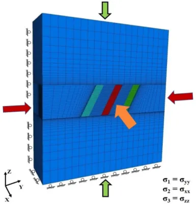
The finite difference code FLAC3D [28] is employed to build models based on the geometry setup obtained by Monte-Carlo simulation (Fig. 4). The transverse stope configuration [12] is selected to generate planar symmetrical models, with multiple neighboring primary stopes having identical dimensions. Stopes are excavated in sequence. The rib pillar W/H ratio is set at 0.4 for all the models according to a database reported by Hudyma [35] that contains 135 rib pillar size parameters observed from 17 different Canadian open stope mines. Different mesh sizes are tested to obtain the most reliable and accurate numerical results. To increase accuracy, a finer mesh size is adopted near the stopes and pillars, while the coarser mesh is applied for the homogeneous isotropic rock mass surrounding the area of interest. To avoid any adverse effect on the obtained results, the roller conditions for external boundaries are positioned far enough from the region of interest, based on different stope dimensions for each model. The identical in situ stress state is applied to the models of all geometrical categories using the magnitudes reported in Table 3. The stopes in each model are excavated in separate single steps from left to right, and after each excavation step, the model is allowed to reach equilibrium.
Figure 4- Model boundary conditions and the state of in situ stress. 3. Results and discussion
The POF is calculated for each class of hanging wall dip in all categories of hanging wall HR for the two considered failure modes. The possibility of brittle failure for each model is evaluated by plotting BSR contours and determining the zone with maximum BSR value (Fig. 5); and the possibility of structurally-controlled gravity driven failure is assessed by comparing the highest magnitude of minimum principal induced stress of each model (as an output of FLAC3D), with the obtained value of rock mass tensile strength (Fig. 6 a–b). The ratio of the number of failed model realizations, over 100 realizations for each hanging wall dip class, provides the POF in percentage. It should be noted that for the presumed state of in situ stress and rock mass quality, no brittle failure condition is observed. Thus, the main failure mechanism is determined to be the structurally-controlled gravity driven (i.e. tensile) failure.
Figure 5- Contour of the brittle shear ratio (BSR).
(a) (b)
Figure 6- Contour of (a) minimum principal induced stress – σ3 (MPa), (b) minimum principal induced stress – σ3 ≥ 0.
In order to have a better understanding about the way each input parameter affects the POF, and/or whether interaction effect exists between the parameters or not, a general factorial design with 36 experiments is generated by Design Expert 7.0 [36] trial software. The general (multi-level) factorial design allows categorical factors to be defined with different numbers of levels and
experiment design and the values of response (POF), obtained from numerical modellings, are presented in Table 5. The process takes place by fitting different regression models (i.e., mean, main effects, 2FI and 3FI) to the response data (POFs). Consequently, ANOVA is used to determine the level of significance for the applied regression models. The final equation (Eq. 12) expresses the relationship between the POF value (response variable), and the individual/interactive effects of independent variables:
( )
[ ] [ ] [ ] [ ] [ ] [ ] [ ] [ ] [ ] [ ] [ ] [ ] [ ] [ ] [ ]
[ ] [ ] [ ] [ ] [ ] [ ] [ ] [ ] [ ] [ ] [ ] [ ]
% ƒ 1 , 2 , 1 , 2 , 3 , 1 , 2 , 1 1 , 2 1 , 1 2 , 2 2 , 1 1 , 2 1 , 3 1 , 1 2 , 2 2 , 3 2 ( ) POF A A B B B C C A C A C A C A C B C B C B C B C B C B C = (12)Where POF is the “probability of failure” in percentage; A, B and C refer to the coded values of stope span width, stope hanging wall dip and stope hanging wall HR, respectively; [n] represents the corresponding level (range) for each input variable.
Table 5- The 36-full factorial experimental runs and the corresponding values of POF obtained from numerical modellings.
Run Span width (m) HW dip (°) HW HR (m) POF (%)
1 8 75-90 7-10 49 2 8 45-60 7-10 47 3 8 60-75 2.5-5 21 4 4 75-90 7-10 14 5 4 60-75 5-7 26 6 8 60-75 7-10 36 7 4 60-75 7-10 6 8 8 60-75 5-7 49 9 4 45-60 7-10 26 10 4 45-60 5-7 32 11 8 20-45 5-7 43 12 4 60-75 2.5-5 23 13 12 75-90 7-10 56 14 8 45-60 2.5-5 55 15 12 60-75 5-7 45 16 8 20-45 2.5-5 36 17 12 45-60 2.5-5 76 18 8 45-60 5-7 34
19 12 20-45 7-10 36 20 4 20-45 2.5-5 28 21 4 20-45 7-10 15 22 12 75-90 2.5-5 50 23 8 75-90 5-7 59 24 12 75-90 5-7 64 25 12 45-60 5-7 37 26 12 60-75 7-10 50 27 8 20-45 7-10 29 28 12 20-45 2.5-5 47 29 12 45-60 7-10 47 30 12 20-45 5-7 40 31 4 45-60 2.5-5 48 32 4 75-90 5-7 42 33 8 75-90 2.5-5 44 34 12 60-75 2.5-5 25 35 4 20-45 5-7 36 36 4 75-90 2.5-5 34
ANOVA results of the general factorial design are presented in Table 6. The applied regression model is statistically significant (p ≤ 0.0001), and the parameter “adequate precision” which reflects the signal to noise ratio [38], has the value well above the minimum desirable limit of 4.0 (Table 7).
Table 6- ANOVA results of the regression model applied to POF data.
Source Sum of
squares
Degree of freedom
Mean
square F-value p-value
Model 6823.97 17 401.41 10.61 < 0.0001 A 2602.06 2 1301.03 34.39 < 0.0001 B 1433.64 3 477.88 12.63 0.0001 C 427.56 2 213.78 5.65 0.0125 AC 613.61 4 153.40 4.05 0.0162 BC 1747.11 6 291.19 7.70 0.0003 Residual 681.00 18 37.83 Cor total 7504.97 35
model is the proximity of the predicted determination coefficient (R2) value and the adjusted R2 (R2adj), which indicates that unnecessary variables are eliminated from the model. If the values of these two parameters fall within approximately 0.20 of each other, a reasonable agreement would be achieved (Table 7).
Table 7- The values of determination coefficient (R2), adjusted and predicted determination coefficients.
Adequate
precision R
2 Adjusted R2 Predicted R2
14.0 0.91 0.82 0.64
Regression coefficient values reflect the way each independent variable impacts the response variable; however, it should be noted that in the case of a general factorial design with multi-level categorical factors, these coefficients do not imply a physical meaning. Since these coefficients are calculated according to a mathematical algorithm, it is strongly recommended [37] to use the model graphs, instead of coefficient values, to develop a better interpretation of the model. Significant model terms influencing the POF are individual parameters of A (span width), B (hanging wall dip), C (hanging wall HR) and interactions of A*C and B*C (Table 6).
3.1. Effect of open stope hanging wall HR on the probability of failure
Dimensions of the stope hanging wall “exposed surface” is one of the most important factors influencing the hanging wall stability, since it directly contributes to the extent of the hanging wall relaxation zone [26]. The stope strike length and height characterize the exposed surface of a hanging wall. According to previous studies [10] [20] [21] longer strike lengths cause a greater degree
of relaxation-related dilution, whereas, decreasing the strike length provides more stability. It is also reported [10] [16] [18] that increasing the stope height contributes to greater instabilities and according to Henning [19], even imposes a stronger effect on hanging wall overbreak, compared to the strike length. Furthermore, to account for the combined effect of hanging wall size and shape, the hydraulic radius (HR) is used as a common measure, and as reported by many studies, increasing the hanging wall HR leads to a higher extent of hanging wall instability [12] [26] [23]. Despite the aforementioned assumptions corresponding to the effect of hanging wall size and shape on stability, the actual role of hanging wall HR has not been fully understood yet, since the interferences caused by variation of other stope geometric parameters such as span width and hanging wall dip have been largely underestimated. Therefore, the effect of the stope hanging wall HR is investigated for three categories of stope with different values of span width; each category contains model realizations with four different classes of hanging wall dip. Figures. 7 a–d illustrate the POFs corresponding to HR variations for each stope hanging wall dip class.
(a) (b) 0 10 20 30 40 50 2.5-5 5-7 7-10 P ro b . o f fa il u re (% ) Hanging wall HR (m) HW Dip 20-45 (°)
Span width 4m Span width 8m
Span width 12m 0 20 40 60 80 2.5-5 5-7 7-10 P ro b . o f fa il u re (% ) Hanging wall HR (m) HW Dip 45-60 (°)
Span width 4m Span width 8m
(c) (d)
Figure 7- POF plots for hanging wall HR variations for three average span width groups. (a) hanging wall dip range 20-45°; (b) hanging wall dip range 45-60°; (c) hanging wall dip range 60-75°; (d) hanging wall dip range 75-90°.
In the case of shallow dipping stopes having hanging wall dip ranging between 20-45°, and span width between 4 m and 8 m, increasing the hanging wall HR range from 2.5-5 m to 5-7 m increases the POF from 30% to 32%, and from 36% to 44%, respectively. Whereas, increasing the HR to its ultimate range (7-10 m), decreases the POF dramatically to 8% and 33%, respectively. However, for stopes with 12 m of span width, increasing the hanging wall HR range, causes the POF to reduce from 46% to 40% (Fig. 7a).
For shallow to moderately dipping stopes (45-60°), with a span width equal to 8 m and 12 m, increasing the hanging wall HR range from 2.5-5 m to 5-7 m, decreases the POF from 58% to 38% and from 69% to 39%, respectively, while increasing the HR to its maximum range (7-10 m), increases the POF to 46% and 53%. However, stopes having span width equal to 4 m became more stable by increasing the hanging wall HR range, resulting in a decrease of the POF from 52% to 21% (Fig. 7b).
In the case of moderately to steeply dipping stopes (60-75°) with a span width of 4 m, increasing the hanging wall HR range from 2.5-5 m to 5-7 m, significantly increases the POF (from 16% to
0 10 20 30 40 50 2.5-5 5-7 7-10 P ro b . o f fa il u re (% ) Hanging wall HR (m) HW Dip 60-75 (°)
Span width 4m Span width 8m
Span width 12m 0 10 20 30 40 50 60 70 2.5-5 5-7 7-10 P ro b . o f fa il u re (% ) Hanging wall HR (m) HW Dip 75-90 (°)
Span width 4m Span width 8m
32%), while increasing the hanging wall HR to its highest range (7-10 m), causes a rapid reduction in the POF (decreased to 12%). For the stopes with a span width equal to 8 m, the POF increases first (from 21% to 44%) by increasing the range of hanging wall HR from 2.5-5 m to 5-7 m, and then decreases to 37% while HR reaches its maximum range (7-10 m). In addition, 12 m-wide stopes have their POF continuously increasing (from 32% to 44%), by increasing the hanging wall HR range (Fig. 7c).
Finally, increasing the range of hanging wall HR from 2.5-5 m to 5-7 m for steeply dipping (75-90°) stopes increases the POF from 35% to 47%, 41% to 59% and 52% to 60%, for span width of 4 m, 8 m and 12 m, respectively, while increasing the HR range to 7-10 m, causes the POF to decrease to 21%, 46% and 53%, for span widths of 4 m, 8 m and 12 m, respectively (Fig. 7d). The obtained results of the stope hanging wall HR effect on the POF, challenges the conventional previous assumptions, since hanging wall HR variation does not show similar patterns of effect depending on differences in span width and hanging wall dip ranges. Thus, these observations strongly suggest the presence of significant interaction effects between hanging wall HR and the two other aforementioned parameters.
3.2. Effect of open stope span width on the probability of failure
The effect of open stope span width on relaxation-related dilution has previously been investigated by some studies, and accordingly as a general notion, it is reported that narrower stopes undergo a larger extent of dilution and therefore are more prone to be unstable [21-22]. However, to obtain a clearer understanding about the effect of span width on stope stability, a more comprehensive assessment is accomplished by considering the influence of other geometric parameters in different ranges.
Figures. 8 a–c plot the effects of stope span width on the POF for three hanging wall HR categories in different hanging wall dip classes. As observed in Figure. 8a, stopes whose hanging wall HR ranges between 2.5 and 5 m, increasing the span width from 4 m to 12 m continuously increases the POF for all four hanging wall dip classes respectively from 30% to 46%, 52% to 69%, 16% to 32% and 35% to 52%. Where stopes had their hanging wall HR range between 5-7 m, increasing span width from 4 m to 8 m raises the POF in all four classes of hanging wall dip, respectively from 31% to 44%, 26% to 38%, 32% to 44% and 47% to 59%; whereas, increasing span width to 12 m causes almost no change in the values of POF for neither of the four hanging wall dip classes. It is also found that stopes with hanging wall dip ranges of 20-45° and 60- 75° have almost identical POFs in every stope span width category (Fig. 8b). Finally, increasing the span width from 4 m to 12 m for the large stopes with a hanging wall HR range of 7-10 m, increases the POF from 8% to 40%, 21% to 53%, 12% to 44% and 21% to 53%, respectively, for hanging wall dip classes of 20- 45°, 45- 60°, 60- 75° and 75- 90°. Here, almost identical POF values are observed in hanging wall dip classes of 45-60° and 75- 90° (Fig. 8c). The results of the stope span width effect on the POF, do not support the previous reported assumptions, since wider stopes show less stability (in terms of POF) than narrower ones.
(a) (b)
(c)
Figure 8- POF plots for span width variations for four hanging wall dip classes. (a) hanging wall HR range 2.5-5 m; (b) hanging wall HR range 5-7 m; and (c) hanging wall HR range 7-10 m.
3.3. Effect of open stope hanging wall dip on the probability of failure
According to Henning [19], greater hanging wall overbreak occurs for shallower dips, since vertical stresses (σ3) are shed onto the surrounding orebody, leading to the creation of larger relaxation zones. Hence, shallow dipping stopes are considered to be more unstable. However, the effect of hanging wall dip may be altered when it is combined with the effect of other stope geometric parameters. 0 20 40 60 80 4 8 12 P ro b . o f fa il u re (% ) Span width (m) Hanging wall HR 2.5-5 (m) HW dip 20-45 (°) HW dip 45-60 (°) HW dip 60-75 (°) HW dip 75-90 (°) 0 20 40 60 80 4 8 12 P ro b . o f fa il u re (% ) Span width (m) Hanging wall HR 5-7 (m) HW dip 20-45 (°) HW dip 45-60 (°) HW dip 60-75 (°) HW dip 75-90 (°) 0 10 20 30 40 50 60 4 8 12 P ro b . o f fa il u re (% ) Span width (m) Hanging wall HR 7-10 (m) HW dip 20-45 (°) HW dip 45-60 (°) HW dip 60-75 (°) HW dip 75-90 (°)
The impacts of open stope hanging wall dip on the POF are presented in Figures. 9 a–c, with three values of span width, in various categories of hanging wall HR ranges. In stopes with a hanging wall HR in the range 2.5-5 m, increasing the hanging wall dip results in similar variation trends on the POF for all the span width groups. Accordingly, for stopes with span widths of 4 m, 8 m and 12 m, increasing the range of hanging wall dip from 20-45° to 45-60°, increases the POF from 30% to 52%, from 35% to 58% and from 46% to 69%, respectively. Moreover, increasing the hanging wall dip to the range of 60-75°, causes a significant decrease in the POF to 16%, 21% and 32%, respectively. Ultimately, reaching a hanging wall dip range of 75-90°, results in 35%, 41% and 52% of POF for stopes with span widths of 4 m to 12 m, respectively (Fig. 9a).
In the case of stopes having hanging wall HR ranging from 5 to 7 m, similar patterns of POF variation are observed for all the span width groups, especially for span widths of 8 m and 12 m, in which almost identical POFs are obtained for each hanging wall dip range. For stopes with a span width equal to 4 m, increasing the range of hanging wall dip from 20-45° to 45-60°, decreases the POF from 31% to 26%, while increasing the hanging wall dip range to 60-75° and ultimately 75-90°, increases the POF to 47%. For stopes with 8 m and 12 m span widths, POFs of 44%, 39%, 44.3% and 59% are obtained for dip ranges of 20-45° to 75-90°, respectively (Fig. 9b).
The effect of increasing the hanging wall dip on the POF shows a similar pattern for all three span width groups with 7-10 m hanging wall HR. Thus, for stopes having span widths of 4 m, 8 m and 12 m, increasing the range of hanging wall dip from 20-45° to 45-60°, increases the POF from 8% to 21%, from 33% to 46% and from 40% to 53% respectively. Moreover, increasing the hanging wall dip range to 60-75°, reduces the POFs to 12%, 37% and 44% respectively. Ultimately, increasing the dip range to 75-90°, results in POFs of 21%, 46% and 53% for span width groups of 4 m to 12 m, respectively (Fig. 9c).
(a) (b)
(c)
Figure 9- POF plots for hanging wall dip variation for three span width groups. (a) hanging wall HR range 2.5-5 m; (b) hanging wall HR range 5-7 m; (c) hanging wall HR range 7-10 m.
3.4. Interaction effect of open stope geometric and inclination parameters on the
probability of failure 0 10 20 30 40 50 60 70 80 20-45 45-60 60-75 75-90 P ro b . o f fa il u re (% )
Hanging wall dip (°)
Hanging wall HR 2.5-5 (m)
Span width 4m Span width 8m
Span width 12m 15 25 35 45 55 65 20-45 45-60 60-75 75-90 P ro b . o f fa il u re (% )
Hanging wall dip (°)
Hanging wall HR 5-7 (m)
Span width 4m Span width 8m
Span width 12m 0 10 20 30 40 50 60 20-45 45-60 60-75 75-90 P ro b . o f fa il u re (% )
Hanging wall dip (°)
Hanging wall HR 7-10 (m)
Span width 4m Span width 8m
As indicated by the results for individual parameters in previous sections, the POF is significantly controlled by strong interactions between certain geometrical parameters. The presence of synergistic effects between the geometrical parameters complicates a general conclusion on the influence of stope size, shape and inclination on the POF. Based on the results of previous studies, it can be assumed that stopes, either with high vertical and short horizontal dimensions or with long horizontal and short vertical dimensions, are considered more stable in comparison to square-shaped stopes [12].
Figures. 10 a–d illustrate the interaction effects of stope span width and stope hanging wall HR, for the hanging wall dip ranges of 20-45°, 45-60°, 60-75° and 75-90° respectively. As previously discussed, it is observed that regardless of the stope hanging wall dip range, increasing the stope span width increases the POF for all three hanging wall HR categories (Figs. 10 a–d).
In shallow dipping stopes (HW dip between 20-45°), increasing the hanging wall HR for stopes with low and moderate span widths (4 m and 8 m), firstly elevates the POF and then reduces the POF to their minimums. However, for large span widths (12 m), a global decreasing trend of POF is observed (Fig. 10a). The most stable condition (POF = 8%) occurs with narrow stopes (span width of 4 m), having the maximum range of hanging wall HR (5-7 m). In contrast, when the horizontal dimensions of the stope becomes closer to its vertical dimension (the category of span width equal to 12 m and HR ranges between 2.5 and 5 m), the POF increases to its maximum level of 46%.
(a) (b)
(c) (d)
Figure 10- General factorial analysis plots showing interaction effects between stope span width and stope hanging wall HR in (a) hanging wall dip range 20-45°; (b) hanging wall dip range 45-60°; (c) hanging wall dip range 60-75°; (d) hanging wall dip range 75-90°.
For shallow to moderately dipping stopes (HW dip between 45-60°) with the span width of 4 m; increasing the hanging wall HR, sharply decreases the POF. In this case, the most stable condition occurs in the group of stopes with span widths of 4 m and hanging wall HR between 7 and 10 m. For stopes with span widths of 8 m and 12 m, increasing the HR decreases the POF in the beginning (at HR range of 5-7 m), and then increases it considerably for larger HR values. It is also observed that reducing the difference between stope’s horizontal and vertical dimensions (the category of span width equal to 12 m and HR ranges between 2.5 and 5 m), results in the most unstable condition in terms of POF (69%) (Fig. 10b).
In the case of moderately to steeply dipping stopes (HW dip between 60-75°), increasing the hanging wall HR first increases the POF (at HR range of 5-7 m), and then decreases it for all the span width categories. Again, the most stable condition in term of POF (11%) is achieved for stopes with hanging wall HR between 7 and 10 m and span width of 4 m (Fig. 10c).
A similar pattern of POF variation is observed for steeply dipping stopes (HW dip between 75-90°), in that increasing the hanging wall HR first increases the POF (at HR range of 5-7 m), and then decreases it across all span widths. In addition, the lowest POF (21%) was observed for stopes with high vertical (HR ranges between 7 and 10 m), and short horizontal (span width of 4 m) dimensions (Fig. 10d).
Across the hanging wall dip classes, the highest level of stability (the lowest POF values), is achieved for the category of stopes with the hanging wall HR ranging between 7-10 m, and span width of 4 m. This result supports the previously stated assumption that high vertical and short horizontal dimensioned stopes are more stable than square-shaped stopes. Moreover, it provides a general pattern for POF variations; where in all the hanging wall dip classes (except the dip class of 45-60°), increasing the hanging wall HR and span width simultaneously, causes the POF to increase. In stopes dipping between 45-60°, increasing the hanging wall HR and span width simultaneously, at first causes the POF to decrease significantly, and then to increase by the same value.
The interaction effect of stope hanging wall HR and stope hanging wall dip, for span widths of 4 m, 8 m and 12 m are presented in Figures. 11 a–c, respectively. Regardless of the stope span width, the POF for the stopes with hanging wall HR ranges between 2.5 and 5 m and 7 and 10 m, follows an increase/decrease/increase pattern as the stope hanging wall dip range is increased. While for
the stopes with a hanging wall HR range of 5-7 m, the POF decreases at first and then continuously increases with increasing stope hanging wall dip ranges (Figs. 11 a–c).
(a) (b)
(c)
Figure 11- General factorial analysis plots showing interaction effects between stope hanging wall dip and stope hanging wall HR for (a) span width of 4 m; (b) span width of 8 m; (c) span width of 12 m.
Where stope span widths equaled 4 m, the POF for the stopes with hanging wall dip ranges of 20-45°, 60-75° and 75-90°, increases to its highest level by increasing the hanging wall HR range from 2.5-5 m to 5-7 m. Consequently, the POF decreases to its minimum when the hanging wall HR is increased to 7-10 m range. However, for stopes with hanging wall dip ranges of 45-60°, the POF continuously decreases with increasing hanging wall HR ranges (Fig. 11a).
For 8 m-wide stopes with moderate to steeply dipping hanging walls (60-75° and 75-90°), increasing the HR range from 2.5-5 m to 5-7 m, increases the POF from their minimum value to their maximum value; however, when HR range is increased to 7-10 m, the POF decreases. For a hanging wall dip range of 20-45°, increasing the HR range to 5-7 m results in an increase of POF to its maximum value, while at the 7-10 m range of HR, the POF is decreased to its minimum value. POF for the stopes dipping between 45-60°, decreases from their maximum to minimum value by increasing the HR from 2.5-5 m to 5-7 m and increases when HR ranges between 7 and 10 m (Fig. 11b).
Finally, for 12 m-wide stopes dipping between 60-75° and 75-90°, increasing the hanging wall HR range from 2.5-5 m to 5-7 m, enhances the POF from their minimum to the maximum value; whereas increasing HR to 7-10 m, causes the POF to decrease. The POF for stopes dipping between 45-60°, decreases from their maximum to minimum values by increasing the HR from 2.5-5 m to 5-7 m; in contrast, an increase in the POF value is observed, when the HR reaches the 7-10 m range. In stopes dipping 20-45°, increasing the HR range from 2.5-5 m to 7-10 m, decreases the POF (Fig. 11c).
4. Conclusions
The Monte-Carlo simulation approach combined with the finite difference code FLAC3D, are employed to assess the individual effects of open stope size, shape and inclination on the stope probability of failure. The effect of stope hanging wall HR, stope span width and stope hanging wall dip were evaluated for three groups of stopes, having different average values of span width (4 m, 8 m and 12 m), with every group divided in three hanging wall HR categories (2.5-5 m, 5-7
m and 7-10 m) and each category of HR varied the hanging wall dip in four classes of 20-45°, 45-60°, 60-75° and 75-90°. In order to calculate the POF as the response variable, the possibility of rock mass brittle failure and structurally-controlled gravity driven (tensile) failure were assessed for simulated stopes through the BSR parameter and the minimum principal induced stress, respectively. It was found that under the presumed state of in situ stress and rock mass quality; structurally-controlled gravity driven failure is the dominant mode of failure. Due to the presence of strong interaction effects between the parameters; a general multi-level factorial design with 36 experiments was utilized to determine the induvial and interactive effects of the parameters. An appropriate quadratic model with an adequate fit was applied to the obtained POF results. The mathematical relationship between the POF and the geometrical parameters in their corresponding levels were adequately described by a polynomial equation. Results indicated that the three parameters stope hanging wall HR, stope span width and stope hanging wall dip have a strong influence on the stope stability state; while the probability of stope failure is significantly controlled by interaction effects between span width / hanging wall HR and hanging wall dip / hanging wall HR. The interaction between the parameters, alters the way each parameter affects the probability of stope failure; hence, the effect of each geometrical parameter on POF must be assessed by considering the variation level of other parameters. However, a key finding of this study is that whatever the stope hanging wall dip is, increasing the stope span width from 4 m to 12 m, increases the POF in all categories of stope hanging wall HR.
Moreover, aside from stope span width range, when the hanging wall HR ranged between 2.5-5 m, the most unstable condition occurs for hanging wall dip between 45-60°, while the most stable condition occurs for hanging wall dip between 60-75°. In contrast, for stopes having their hanging
wall HR ranging between 5-7 m, the most stable condition occurs for the hanging wall dip range of 45-60°, while the maximum instability is observed for hanging wall dip between 75-90°. Furthermore, it can be concluded that independent of stope span width, increasing the stope hanging wall HR range from 2.5-5 m to 7-10 m decreases the POF for the stopes dipping up to 60°. While stopes dipping greater than 60°, the most unstable condition occurs for the hanging wall HR range of 5-7 m for all span width groups.
The mathematical optimization performed with Design Expert 7.0 [36] trial software predicts that the maximum stability (in terms of POF) would be achieved for narrow stopes (span width of 4 m) whose hanging wall dip ranges between 20 and 45° and hanging wall HR ranges between 7 and 10 m. In contrast, the maximum instability would occur in wider stopes (span width equal to 12 m) whose hanging wall HR ranges between 2.5-5 m and hanging wall dip ranges between 45 and 60°.
Acknowledgements
This work was funded by a grant from Natural Sciences and Engineering Research Council of Canada (NSERC) and the authors would like to acknowledge the Niobec mine (Saint-Honoré, Québec).
References
1. Hudson JA. Comprehensive Rock Engineering: Principles, Practice & Projects. Vol 5. Pergamon Press; Oxford, United Kingdom, 1993.
2. Wang J. Influence of stress, undercutting, blasting, and time on open stope stability and dilution. PhD thesis, University of Saskatchewan, Saskatoon, Canada, 2004.
3. Zhang Y, Mitri HS. Elastoplastic stability analysis of mine haulage drift in the vicinity of mined stopes. Int J Rock Mech Min Sci. 2008; 45(4):574–593.
4. Abdellah W, Raju GD, Mitri HS, Thibodeau D. Stability of underground mine development intersections during the life of a mine plan. Int J Rock Mech Min Sci. 2014; 72:173–181.
5. Einstein HH. Risk and risk analysis in rock engineering. Tunneling and Underground Space Technology 1996; 11 (2):141–55.
6. Brown ET. Risk assessment and management in underground rock engineering—an overview. Journal Rock Mech Geotech Eng.; 2012(3):193–204.
7. Idris MA, Saiang D, Nordlund E. Probabilistic analysis of open stope stability using numerical modelling. Int. J. Min. Miner. Eng. 2011; 3(3):194–219.
8. Diederichs MS, Kaiser PK. Rock instability and risk analyses in open stope mine design. Can Geotech J. 1996; 33(3):431–439.
9. Chen G, Jia Z, Ke J. Probabilistic analysis of underground excavation stability. Int. J. Rock Mech. & Min. Sci. 1997; 34:3–4, paper No. 051.
10. Henning JG, Mitri HS. Numerical modelling of ore dilution in blasthole stoping. Int J Rock Mech Min Sci. 2007; 44:692–703.
11. Idris MA, Basarir H, Nordlund E, Wettainen T. The Probabilistic Estimation of Rock Masses Properties in Malmberget Mine, Sweden. Electron J Geotech Eng. 2013; 18:269–287.
12. Villaescusa E. Geotechnical design for sublevel open stoping. CRC Press. New South Wales, Australia, 2014.
13. Aglawe JP. Unstable, violent failure around underground openings in highly stressed ground. PhD thesis, Queen’s University at Kingston, Ontario, Canada 1999.
14. Castro LAM, Bewick RP, Carter TG. An overview of numerical modelling applied to deep mining. In: Azevedo R, editor. Innovative numerical modelling in geomechanics. London: CRC Press — Taylor & Francis Group; 2012. p. 393–414.
15. Idris MA. Probabilistic stability analysis of underground mine excavations. PhD thesis, Lulea University of Technology, Lulea, Sweden, 2014.
16. Chen D, Chen J, Zavodni ZM. Stability analysis of sublevel open stopes at great depth. The 24th U.S. Symposium on Rock Mechanics (USRMS), 1983.
17. Perron, J. Simple solutions and employee’s involvement reduced the operating cost and improved the productivity at Langlois mine. Proceeding 14th CIM Mine Operator’s Conference. Bathurst, New Brunswick, Canada, 1999.
18. Yao, X., G. Allen, et al. Dilution evaluation using the cavity monitoring system at HBSM-Trout Lake Mine. 101th Annual General Meeting, Calgary, Canada, 1999.
19. Henning JG. Evaluation of Long-Hole Mine Design Influences on Unplanned Ore Dilution. PhD thesis, McGill University, Montreal, Canada, 2007.
20. Hughes R. Factors influencing overbreak in narrow vein longitudinal retreat mining. MSc thesis. McGill University, Montreal, Canada, 2011.
21. El Mouhabbis HZ. Effect of stope construction parameters on ore dilution in narrow vein mining. MSc thesis. McGill University, Montreal, Canada, 2013.
22. Pakalni RC, Poulin R, Hadjigeorgiou J. Quantifying the cost of dilution in underground mines. Mining Eng 1995; Dec: 1136–41.
23. Urli V. Ore-Skin Design to Control Sloughage in Underground Open Stope Mining. MSc thesis. University of Toronto, Toronto, Canada. 2015.
24. Milne D. Underground design and deformation based on surface geometry. PhD Thesis, Mining Department, University of British Columbia, Vancouver, Canada, 1996.
25. Germain P, Hadjigeorgiou J. Influence of stope geometry and blasting patterns on recorded overbreak. Int J rock Mech Min Sci. 1997; 34(3–4):628.
26. Clark L. Minimizing dilution in open stope mining with a focus on stope design and narrow vein longhole blasting. MSc thesis, University British Columbia, Vancouver, Canada, 1998.
27. Wang J, Milne D, Wegner L, Reeves M. Numerical evaluation of the effects of stress and excavation surface geometry on the zone of relaxation around open stope hanging walls. Int J Rock Mech Min Sci. 2007; 44(2):289–298.
28. Itasca Consulting Group, Inc. 2012. FLAC3D – Fast Lagrangian Analysis of Continua in 3 Dimensions, Ver. 5.0, User’s Guide. Minneapolis: Itasca, USA.
29. Hoek E. Practical rock engineering.Asp, 2000, World Wide Web edition.
30. Arjang B, Herget G. In situ ground stresses in the Canadian hard rock mines: an update. Int J Rock Mech Min Sci 1997; 34: paper 015.
31. Maloney S, Kaiser P, Vorauer A. A re-assessment of in situ stresses in the Canadian Shield. InGolden Rocks 2006, The 41st US Symposium on Rock Mechanics (USRMS) 2006 Jan 1. American Rock Mechanics Association.
32. Diederichs MS. Instability of hard rock masses: the role of tensile damage and relaxation. PhD thesis, University of Waterloo, Canada, 1999.
33. Shnorhokian S, Mitri HS, Moreau-verlaan L. Stability assessment of stope sequence scenarios in a diminishing ore pillar. Int J Rock Mech Min Sci. 2015; 74:103–118.
34. Kaiser PK, Diederichs MS, Martin CD. Underground works in hard rock tunneling and mining. In: GeoEng2000, Proceedings of the International Conference on Geotechnical and Geological Engineering, Melbourne, Australia, 2000.
35. Hudyma MR. Development of empirical rib pillar design criterion for open stope mining. PhD thesis, University of British Columbia. Vancouver, Canada, 1988.
36. Stat-Ease, Inc. 2005. Design-Expert 7.0.0 Minneapolis, USA.
37. Design-Expert 7.0.0 Manual. Stat-Ease, Inc. 2005. Minneapolis, USA.
38. Ahmadi A, Heidarzadeh S, Reza A, Darezereshki E, Asadi H. Optimization of heavy metal removal from aqueous solutions by maghemite ( γ -Fe 2 O 3 ) nanoparticles using response surface methodology. J Geochemical Explor. 2014; 147:151–158.


![Figure 2- An open stope geometrical parameters (Adopted from Wang [2]).](https://thumb-eu.123doks.com/thumbv2/123doknet/7488238.224244/10.918.212.703.225.603/figure-open-stope-geometrical-parameters-adopted-wang.webp)