Xanthomonas
oryzae pv. oryzae
CASE STUDY
OF THE SPECIFIC
PHYTOSANITARY
SURVEILLANCE SYSTEM
Surveillance System: case study: Xanthomonas oryzae pv. oryzae by IICA is published under license Creative Commons
Attribution-ShareAlike 3.0 IGO (CC-BY-SA 3.0 IGO) (http://creativecommons.org/licenses/by-sa/3.0/igo/)
Based on a work at www.iica.int
Montevideo, Uruguay 2018 DEWEY 632.32 AGRIS H20
IICA encourages the fair use of this document. Proper citation is requested.
This publication is available in electronic (PDF) format from the Institute's Web site: http://www.iica.int
Editorial coordination: Lourdes Fonalleras and Florencia Sanz Translator: Paula Fredes
Layout: Victor Hugo Vidart Cover design: Victor Hugo Vidart Digital printing
Guidelines for the implementation of the Specific Phytosanitary Surveillance System: case study: Xanthomonas oryzae pv. oryzae / Inter-American Institute for Cooperation on Agriculture, Comité Regional de Sanidad Vegetal del Cono Sur; José Manuel Galarza. – Uruguay : IICA, 2018. A4; 21 cm x 29,7 cm.
ISBN: 978-92-9248-787-4 Published also in Spanish
1. Plant diseases 2. Xanthomonas oryzae 3. Crops 4. Rice 5. Disease surveillance 6. Risk management 7. Weeds 8. Environmental factors 9. Cartography I. IICA II. COSAVE III. Title.
Pablo Cortese, Ignacio García Varona, Federico Aguirre, Oscar Von Baczko, Yanina Outi from Servicio Nacional de Sanidad y Calidad Agroalimentaria – SENASA from Argentina;
Luis Sánchez Shimura, Remi Castro Ávila, Gustavo López Zenteno, Edgar Delgado Vargas, Immer Adhemar Mayta Llanos, Geordana Zeballos from Servicio Nacional de Sanidad Agropecuaria e Inocuidad Alimentaria – SENASAG from Bolivia; Ricardo Kobal Raski, Dalci de Jesus Bagolin, Jesulindo de Souza Junior, Ériko Tadashi Sedoguchi from Secretaria de Defensa Agropecuaria del MAPA from Brasil;
Marco Muñoz, Fernando Torres Parada, Jairo Eladio Alegría Contreras, Carolina Pizarro, Karina Reyes, Ilania Astorga from Servicio Agrícola y Ganadero – SAG from Chile;
The Guide for the Implementation of Specific Phytosanitary Surveillance System has been applied through two case studies. Those products were
developed as a result of the component aimed at strengthening plant pest surveillance in the framework of STDF / PG / 502 Project "COSAVE: Regional Strengthening of the Implementation of Phytosanitary Measures and Market Access". The beneficiaries are COSAVE and the NPPOs of the seven countries that make up COSAVE. The Standards and Trade
Development Facility (STDF) fund it, the Inter-American Institute for Cooperation on Agriculture (IICA) is the implementing organization and the IPPC Secretariat supports the project.
The editorial coordination was in charge of Maria de Lourdes Fonalleras and Florencia Sanz.
Maria de Lourdes Fonalleras, Florencia Sanz y José Manuel Galarza, have defined the original structure of this Guide.
The content development corresponds exclusively to José Manuel Galarza expert contracted especially for the project.
The technical readers that made important contributions to develop the study cases are the specialists of the NNPO's participating in the Project:
Bettina Chaparro from Servicio Nacional de Calidad, Sanidad Vegetal y de Semillas – SENAVE from Paraguay; Moisés Pacheco Enciso, Johny Naccha Oyola, Cecilia Lévano Stella, Betty Matos Nonogawa, Carmen Oré Vento, Iván Gutiérrez Martínez, Jorge Velapatiño Flores, Percy Alberto Mamani Sánchez from Servicio Nacional de Sanidad Agraria – SENASA from Perú;
Elina Zefferino and Noelia Casco from Dirección General de Servicios Agrícolas – DGSA/ MGAP from Uruguay.
We express special appreciation to all of them. We also thank the support received from the IPPC
Secretariat for the implementation of this component of the project.
Finally, we thanks Víctor Vidart by diagramming the document.
1.
PURPOSE
Detection surveillance of Xanthomonas oryzae pv. oryzae in rice production and host weeds in the COSAVE region.
2.
SCOPE
COSAVE region, considering pest records and suitable environmental conditions for the pest.
3.
TARGET PEST
Xanthomonas oryzae pv. oryzae, see the pest datasheet in Annex 1.
4.
DURATION AND APPROPRIATE TIMING
The duration is one (1) growing season, during the active growing stage of the crop, with a weekly frequency between surveys.
5.
SITE SELECTION
For the area or site selection process, the following information is required in advance:
• Cadastral map of the region
• Hydrography and geographical characteristics (forests, mountains, lakes, rivers, deserts) in the location
• Risk map for the region
• Area and production of the crop at the political and administrative level as detailed as possible
Fig. 1. Environmental risk map of Xanthomonas oryzae pv. oryzae for the COSAVE region. Higher risk in red, medium risk in yellow and lower risk in light blue. Scale 1:45,000,000. Source: Prepared for STDF/PG/502 COSAVE Project.
Risk maps for the target pest can be managed for the risk characterization and the regional prioritization of surveillance activities. In this study case, we use the MaxEnt model, to identify the environmental risk for Xanthomonas oryzae pv. oryzae with worldwide locations that report the pest and their correlation with the bioclimatic variables from the Worldclim database
(http://www.worldclim.org/). The details of the method appear in Annex 2 and the resulting regional environmental risk map in Figure 1. The areas in red and yellow mean higher and medium risk respectively, light blue means lower estimated risk. The risk estimation is based on
MaxEnt results and the comparison of the presence of the pest and the bioclimatic variables where the pest is reported.
5.1. Environmental modeling for the development of risk maps for the region
The environmental niche modeling is commonly used to develop probabilistic maps of species distribution. Among the available modeling techniques, MaxEnt has become one of the most popular tools for modeling species distribution, with hundreds of peer-reviewed articles published each year. The popularity of MaxEnt is mainly due to the short running time, easy operation, small sample size, high simulation precision, the use of a graphical interface and automatic parameter configuration capacities (Morales et. al, 2017; Costa P., Holtz V. 2011; Wang R. et al. 2018).
Fig. 2. Host risk map—rice in the COSAVE region. High risk in red, medium risk in yellow and low risk in light blue. Scale 1:45,000,000. Source: Prepared for STDF/PG/502 COSAVE Project.
5.2. Host area in the region
Xanthomonas oryzae pv. oryzae hosts
belong to the genus Oryza as well as wild species from the Poaceae and Cyperacea family, as described in the datasheet (Annex 1). Rice production is economically
important in the region. It accounts for about 214,570 hectares in Argentina; 181,497 in Bolivia; 2,162,178 in Brazil; 20,937 in Chile; 167,088 in Peru; 131,740 in Paraguay, and 164,400 hectares in Uruguay. Based on rice production information at a first
administrative-geopolitical level in each COSAVE country, it is possible to develop a host risk map. As Fig. 2 illustrates, the NPPO can determine the levels as high, medium and low based on the importance of
production in each identified administrative-geopolitical level. The method for its
preparation is discussed in Annex 2.
5.3. Regional risk for xanthomonas oryzae pv. oryzae
It is possible to integrate the
environmental and host risk maps in one regional risk map, as is illustrated in Fig. 3. The method is presented in Annex 2 and is based on the reclassification of high-risk category with a value of two (2), medium with one (1) and low with zero (0); and the use of the raster
mathematical multiplication function of a geographic information system like QGIS. The method for its preparation is
described in Annex 2.
Fig. 3. Regional risk map of Xanthomonas oryzae pv. oryzae for COSAVE. High risk in red, medium risk in yellow and low risk in light blue. Scale 1:45,000,000. Source: Prepared for STDF/PG/502 COSAVE Project.
5.4. Selected sites for the surveillance
Considering pest reports, it is necessary to identify the potential considerations for the entry of the pest. In this regard, it is important to identify the main transporting routes and the main rivers that can spread the pest with rice seeds, as well as nearby places of production.
It is possible to integrate the regional risk of the pest and the location of routes and rivers consolidated by the Consejo Suramericano de Infraestructura y Planeamiento (COSIPLAN) (Available at:
http://www.sig.cosiplan.unasursg.org/node/15, on January 5, 2018). For a better management of field actions, the NPPO can identify squares (grids), with the appropriate size to describe a uniform population for the sampling, as shown in Fig. 4 and 5, with 100 km grids. The method for preparation is also described in Annex 2.
Fig. 4. 100 km squares used for the integration of main rivers location and the regional risk information of the pest (high risk in red, medium risk in yellow and low risk in light blue. Scale 1:45,000,000. Source: Prepared for STDF/PG/502 COSAVE Project.
Fig. 5. 100 km squares used for the integration of main routes location and regional pest risk information (high risk in red, medium risk in yellow and low risk in light blue. Scale 1:45,000,000. Source: Prepared for STDF/PG/502 COSAVE Project.
The NPPO can identify risk squares (grids) with a code and review it with
additional information and then identify the appropriate place for the surveillance. In addition, with the rivers and transport routes information, the NPPO can identify the high-risk squares (grids). The number of squares (grids) separated by risk
category is presented in table 1 and 2. This identification should be complemented with additional information from the NPPO.
Table 1. Number of squares (grids) in major rivers by Xanthomonas oryzae pv. oryzae risk level.
ARGENTINA BOLIVIA BRASIL CHILE PERÚ PARAGUAY URUGUAY 13 16 84 113 12 20 19 51 22 196 131 349 1 3 23 27 11 37 28 76 1 3 14 18 10 11 21 60 285 310 655 ARGENTINA BOLIVIA BRASIL CHILE PERÚ PARAGUAY URUGUAY 15 17 242 274 23 24 32 79 38 383 224 645 2 4 75 81 3 18 76 97 2 9 14 25 1 11 14 26 84 466 677 1227
This information is available to open with the QGIS, downloading the complete folder “Qxoo” from the link: https://goo.gl/WYFe6a
Table 2. Number of squares (grids) in major routes by Xanthomonas oryzae pv. oryzae risk level.
COUNTRY HIGH MEDIUM LOW TOTAL
COUNTRY HIGH MEDIUM LOW TOTAL
Source: Prepared for STDF/PG/502 COSAVE Project. Source: Prepared for STDF/PG/502 COSAVE Project.
6.
PLANNING
6.1. Preliminary activities
For a better operational organization, it is necessary to recognize the national characteristics of the risk, places and supplies for surveillance implementation. This allows the NPPO to evaluate, manage and systematize the activity. In this regard, it is important to include the following:
• The annual operating plan with the inclusion of the budget, geographical distribution, task schedule and the implementation time.
• Coordination with the diagnostic laboratory, including the protocol and the number of samples to be submitted.
• Cadastral map of the region.
• Hydrography and geographical characteristics (forests, mountains, lakes, rivers or deserts) in the location.
• Hosts area and production at the administrative-geopolitical level as detailed as possible.
• Phenology of the involved hosts.
• Location of rice seedbeds, collection and storage centers, and risk areas.
• International transport routes.
• Collate pest information in a datasheet like Annex 1. • Manage permissions to enter private property in advance. • Ensure the required supplies and resources for the surveillance. • Training for directly involved staff.
6.2.1. Required supplies
• Disposable cloths and gloves. • Field knife for the sampling. • Alcohol burner.
• Alcohol 70% for hand disinfection. • Bleach 10% for sample collection. • Identification labels.
• Plastic and paper bags for sampling. • Entomological clamps.
• Writing pads. • Pencil.
• Dishcloth for tool cleaning.
• Devices to capture geo-referenced field data. • Templates for data collection.
6.2.2. Sample collection and submission
In case that the visual survey (inspection) can identify Xanthomonas, it is necessary to confirm its identification safeguarding its integrity and
submitting the sample to the laboratory. This official diagnosis requires prior coordination of the number of the samples that can be identified.
6.2. Surveillance methodology
The visual inspection or survey can be an effective surveillance method when the characteristics or symptoms of the pest enable identification, which can be
confirmed with the laboratory diagnosis. Moreover, it is important to consider: • The surveillance of Xanthomonas oryzae pv. oryzae is performed with the
visual inspection or survey in production locations, tissue sampling and pest isolation.
• The number of inspections or surveys can follow the recommendations of the “Guidelines for the implementation of the specific phytosanitary surveillance system”.
• Identification of the varieties and other pest susceptible species. • Ecological conditions that encourage the presence of the pest. • Rice seedbeds.
COUNTRY AND ACTIVITY PLACE HOST AND RESULTS INCIDENCE AND SEVERITY
Item País
Fecha (dd/mm/aaaa) Actividad de Vigilancia Inspección, muestreo, trampeo, otro _______
(especificar)
Coordenadas geográficas decimales: LA
TITUD
Coordenadas geográficas decimales: LONGITUD Hospedante (Citrus sinensis, Citrus reticulata, Citrus unshiu, Citrus aurantifolia, Or
yza sativa,
otro_______ (especificar) Tipo de Predio (Comer
cial,
vivero, traspatio, aislado, otro________(especificar)
Resultado
(Ausente o Presente) Incidencia encontrada Descripción de la
incidencia evaluada(% u otro______ (especificar) Severidad encontrada Severidad (Grados u otro ________(especificar)
Obser vación 1 2 3 4 5 6 7 8 9 10 11 12 13 14 1 2 3 4 5 6 7 8 9 10 11 12
Fig. 6. General template to record Xanthomonas oryzae pv. oryzae surveillance activities. Source: Prepared for STDF/PG/502 COSAVE Project.
In addition, this general template should have modeled fields in order to avoid mistakes in recording information and the use of computing platforms. For example, Open Data Kit is capable of collecting geo-referenced information with Android devices. The details, templates and explanations for its use are available in the ODK folder in the link: https://goo.gl/WYFe6a.
6.3. Recording surveillance activities
In order to collate and implement automated reports, the activities of the information record for the Surveillance System should be performed in a
standardized and integrated manner. In this regard, we present a general template
for the identification of the required information to record Xanthomonas oryzae
pv. oryzae surveillance activities.
6.4. Biosafety
To achieve biosecurity in surveillance actions, it is necessary to include:
• The use of new disposable cloths during the entry to each surveillance site. • The handling of plants or samples should be done with gloves to avoid
contaminating nearby locations.
• Surveillance waste should be kept in properly closed plastic bags. • Any waste material should follow NPPO waste recommendations. • Hand disinfection with approved supplies is required after each activity.
7.
COMMUNICATION
It is important to produce reports with the results of the various level of decision making.
8.
AUDIT
Through the central coordination, each NPPO will perform auditing activities at any stage of the process, analyzing the data in the system, and monitoring the quality of the field tasks performance, among others.
9.
REFERENCES
CABI, 2017. Crop Protection Compendium. Data Base. Wallingford, United Kingdom.
Sheldeman X & van Zonneveld M. 2011. Manual de Capacitación en Análisis Espacial de Diversidad y Distribución de Plantas. Bioversity International, Rome, Italy. 186 pp. Available on October 27, 2017, at:
http://www.bioversityinternational.org/e-library/publications/detail/manual-de-capacitacion-en-analisis-espacial-de-diversidad-y-distribucion-de-plantas/ Singh, R.A., and Rao, M.H.S. 1977. A simple technique for detecting Xanthomonas oryzae in rice seeds. Seed Science and Technology 5: 123-127. Available on October 27, 2017, at: http://download.ceris.purdue.edu/file/289
Wang R, Li Q, He S, Liu Y, Wang M, Jiang G. 2018. Modeling and mapping the current and future distribution of Pseudomonas syringae pv. actinidiae under climate change in China. PLoS ONE 13(2): e0192153. Available on February 26, 2018, at: https://doi.org/10.1371/journal.pone.0192153
10.
ANNEXES
Annex 1. Data sheet of the pest
ANNEX 1
DATA SHEET OF THE PEST
Xanthomonas oryzae pv. oryzae (Ishiyama 1922)
Swings et al. 1990
Synonyms:
Bacterium oryzae (Uyeda & Ishiyama) Nak., 1928; Phytomonas oryzae (Ishiyama) Magrou 1937; Pseudomonas oryzae Ishiyama; Xanthomonas campestris pv. oryzae (Ishiyama 1922) Dye 1978; Xanthomonas itoana (Tachinai) Dowson; Xanthomonas kresek Schure 1953; Xanthomonas oryzae (Ishiyama 1922) Swings et al. 1990; Xanthomonas translucens f. sp. oryzae Jones et al; Dowson; Ishiyama; Pordesimo. Taxonomic rank: Phylum: Proteobacteria Class: Bacteria Order: Xanthomodales Family: Xanthomonadaceae Genus: Xanthomonas
Species: Xanthomonas oryzae pv. oryzae (Ishiyama 1922) Swings et al. 1990 Common names:
Enfermedad bacteriana de las hojas del arroz (spanish); maladie bactérienne des feuilles du riz (french); bacterial leaf blight of rice; kresek disease; rice bacterial leaf blight; rice kresek disease (english).
Hosts:
Cenchrus ciliaris, Cynodon dactylon, Cyperus difformis, Cyperus rotundus,
Echinochloa crus-galli, Leersia hexandra, Leersia oryzoides, Leptochloa chinensis, Megathyrsus maximus, Oryza spp., Oryza longistaminata, Oryza sativa, Paspalum scrobiculatum, Urochloa mutica, Zizania aquatica, Zizania palustris, Zoysia
japonica (CABI, 2017). Geographic distribution:
America: Mexico, United States, Costa Rica, El Salvador, Honduras, Nicaragua, Panama, Colombia, Ecuador, Venezuela (CABI, 2017).
Asia: Pakistan, Philippines, Sri Lanka, Taiwan, Vietnam (CABI, 2017).
Africa: Burkina Faso, Cameron, Egypt, Gabon, Gambia, Madagascar, Mali, Niger, Nigeria, Tanzania, Togo (CABI, 2017).
Europe: Russia (CABI, 2017).
Biology:
Xanthomonas oryzae pv. oryzae survives during the off-season in seed, weed hosts, rice volunteers and infected rice straw and stubble. The evidence for significant seed transmission is contradictory. Survival in soil is limited to a few months at the most in relatively cool, moist conditions (the bacterium dies rapidly in hot, dry conditions) and is thus of little significance in single-crop rice systems. Transmission in irrigation water and floodwater is important during the cropping period, but survival in water is limited to a few days (CABI, 2017).
The bacterium invades rice plants through hydathodes on leaves, root-growth cracks and wounds. Seedling roots are wounded when pulled from the seedbed; and leaf tips are often cut before transplanting. When inside the plant, the bacterium enters the vascular system in which it spreads. Bacteria eventually ooze out of water pores on hydathodes (CABI, 2017).
Signs and symptoms:
The symptoms known as 'kresek' (wilting, desiccation of leaves and death,
characteristic of systemic infection) occur with particular combinations of virulent isolates and susceptible cultivars, probably when the vascular system is blocked by bacterial cells and extracellular polysaccharide. Kresek is associated with tropical storms which spread the pathogen and also wound rice plants. High temperature (30°C) and humidity favor the disease (CABI, 2017).
Fig. 7. Symptoms of Xanthomonas oryzae pv. oryzae due to artificial inoculation (Source: Purdue University, 2017).
Symptoms appear on leaves of young plants, after planting out, as pale-green to grey-green, water-soaked streaks near the leaf tip and margins. These lesions coalesce and become yellowish-white with wavy edges. The whole leaf may eventually be affected, becoming whitish or greyish and then dying. Leaf sheaths and culms of more susceptible cultivars may be attacked. Systemic infection, known as kresek, results in wilting, desiccation of leaves and death, particularly of young transplanted plants. In older plants, the leaves become yellow and then die. In later stages, the disease may be difficult to distinguish from bacterial leaf streak (X. oryzae pv. oryzicola) (CABI, 2017).
The bacteria can only move short distances in infected crops. The bacteria can only move long distances in infected rice seeds. The bacteria are usually found in the glumes, but may also penetrate the endosperm (EPPO, 2003).
Survey (inspection) and detection:
Symptoms appear on leaves of young plants, after planting out, as pale-green to grey-green, water-soaked streaks near the leaf tip and margins. These lesions coalesce and become yellowish-white with wavy edges. The whole leaf may eventually be affected, becoming whitish or greyish and then dying.
Leaf sheaths and culms of more susceptible cultivars may be attacked. Systemic infection, known as kresek, results in wilting, desiccation of leaves and death, particularly of young transplanted plants. In older plants, the leaves become yellow and then die. In later stages, the disease may be difficult to distinguish from X. oryzae pv. oryzicola (CABI, 2017).
Pest impact:
Bacterial leaf blight is the most serious disease of rice in South-East Asia, particularly since the widespread cultivation of dwarf high-yielding cultivars (EPPO, 2003). In Japan, where figures are available, up to 400,000 ha may be affected annually, with losses of 20-30% and up to 50%. In Africa, losses of 2.7-41% in grain yield have been found (CABI, 2017).
In the Philippines, losses are estimated at 22.5% (in wet seasons) and 7.2% (in dry seasons) in susceptible varieties and 9.5 and 1.8%, respectively, in resistant crops (EPPO, 2003).
Pest control and mitigation measures:
Preventive phytosanitary control measures include: • Use of healthy and treated seeds.
• Resistant varieties.
• Careful attention to crop management (for example, water control, avoidance of damage to seedlings) is very important.
• Restricting nitrogen fertilizer applications to about 80-100 kg N/ha. • Chemical control is not recommended (CABI, 2017).
Fig. 8. Infected rice seedlings. Infected leaves wilt and roll up, turning grayish-green to yellow, until the whole seedling dies. Plants which have survived the disease are stunted and yellowish (Picture from EPPO, 2017).
ANNEX 2
Modeling for Xanthomonas oryzae pv. oryzae
A. Data:
This section will discuss the origin and type of data used in the case studies. All the working files, software, references, and other data are available in the link: https://goo.gl/WYFe6a.
A1. Environmental raster data (“*.tif”)
For geo-referenced climate data, go to http://www.worldclim.org/ and then click on Version 2 (http://worldclim.org/version2) for updated climate data.
Fig. 9. Link to Version 2 of the web page: http://www.wordclim.org.
Fig. 10. Download the 10 minutes data.
NOTE: The folder with this data is named “WC10y1990tiff” and is located in the link: https://goo.gl/WYFe6a.
NOTE: The bioclimatic variables are: BIO1 = Annual Mean Temperature, BIO2 = Mean Diurnal Range (Mean of monthly (max temp - min temp)), BIO3 =
Isothermality (BIO2/BIO7) (* 100), BIO4 = Temperature Seasonality (standard deviation *100), BIO5 = Max Temperature of Warmest Month, BIO6 = Min
Temperature of Coldest Month, BIO7 = Temperature Annual Range (BIO5-BIO6), BIO8 = Mean Temperature of Wettest Quarter, BIO9 = Mean Temperature of Driest Quarter, BIO10 = Mean Temperature of Warmest Quarter, BIO11 = Mean
Temperature of Coldest Quarter, BIO12 = Annual Precipitation, BIO13 =
Precipitation of Wettest Month, BIO14 = Precipitation of Driest Month, BIO15 = Precipitation Seasonality (Coefficient of Variation), BIO16 = Precipitation of Wettest Quarter, BIO17 = Precipitation of Driest Quarter, BIO18 = Precipitation of Warmest Quarter, BIO19 = Precipitation of Coldest Quarter.
NOTE: In the link to Version 1.4, we share access to the projected future data for 2050 and 2070, under four (4) scenarios called RCP (“Representative Concentration Pathways”).
Figura 11. Descargar las capas vectoriales y descomprimirlas haciendo un clic con el botón izquierdo del mouse. A2. Vector data (“*.shp”)
The Consejo Suramericano de Infraestructura y Planeamiento (COSIPLAN) collated cartographic information about the following layers in the region:
Border control (CSP_AH070_N), Populated center (CSP_AL105_N), Railway Line (CSP_AN010_L), Railway station (CSP_AN070_N), Main road
(CSP_AP030_L), Port (CSP_BB005_N), Lake (CSP_BH080_P), River (CSP_BH140_L, CSP_BH140_P), Administrative border (CSP_FA000_L), (CSP_FA001_L, CSP_FA001_P), 3er level administrative zone (CSP_FA002_P), Border crossing (CSP_FA125_N), Airport (CSP_GB001_N), and others.
This information is packed in a zip file, available on October 27, 2017 in the link http://www.sig.cosiplan.unasursg.org/node/15, unzip and save the file in a separated folder like DATA in the link: https://goo.gl/WYFe6a.
A3. Geo-referenced data of pests (use of geographic coordinates as an example)
In the CABI Invasive Species Compendium webpage, refer to:
Xanthomonas oryzae pv. oryzae or go to the link:
Go to the lower part of the world distribution map and to the link “Download CSV file” or “Comma separated values” that can be opened with Microsoft Excel.
Fig. 13. Delete the data with the “Absend” or “Restricted distribution” pest situation and arrange the elements as is shown. Fig. 12. Download the CSV (“Comma
separated values”) files.
Open the data in Microsoft Excel, delete the reports of the pest with the situation label as “Absent” or “Restricted distribution” and include first the column species, then longitude and after latitude. Delete the other columns.
Double-check the existence of the species column first, then the longitude and latitude columns respectively and save it as “Xoo.csv” (“Comma separated value”). This data is available in the “cXanthomonasoryzaoryzae” folder in the link:
B. Software:
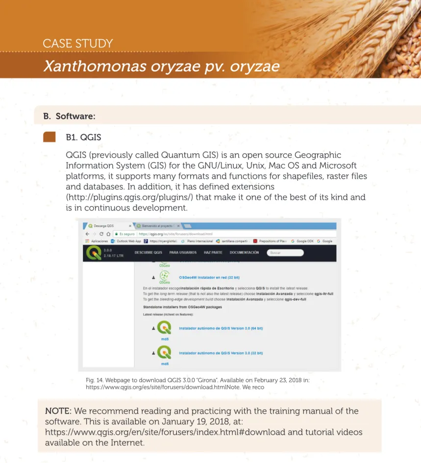
B1. QGIS
QGIS (previously called Quantum GIS) is an open source Geographic Information System (GIS) for the GNU/Linux, Unix, Mac OS and Microsoft platforms, it supports many formats and functions for shapefiles, raster files and databases. In addition, it has defined extensions
(http://plugins.qgis.org/plugins/) that make it one of the best of its kind and is in continuous development.
Fig. 14. Webpage to download QGIS 3.0.0 “Girona”. Available on February 23, 2018 in: https://www.qgis.org/es/site/forusers/download.htmlNote. We reco
NOTE: We recommend reading and practicing with the training manual of the software. This is available on January 19, 2018, at:
https://www.qgis.org/en/site/forusers/index.html#download and tutorial videos available on the Internet.
B2. MaxEnt
B2.1. Installing Java, if not already installed
To verify if Java is installed on your computer, go to the link:
https://www.java.com/es/download/installed.jsp with Internet Explorer To install Java in Internet Explorer, go to the link:
To install Java in Mozilla Firefox, go to the link:
http://www.java.com/en/download/help/firefox_online_install.xml
NOTE: Java is not supported in Google Chrome
B.2.2. Installing MaxEnt
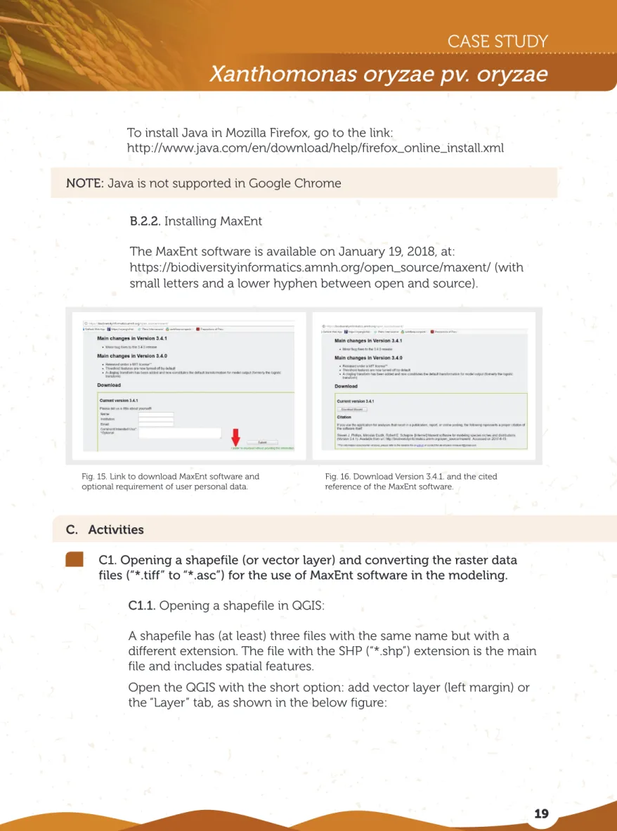
The MaxEnt software is available on January 19, 2018, at:
https://biodiversityinformatics.amnh.org/open_source/maxent/ (with small letters and a lower hyphen between open and source).
Fig. 15. Link to download MaxEnt software and optional requirement of user personal data.
Fig. 16. Download Version 3.4.1. and the cited reference of the MaxEnt software.
C. Activities
C1. Opening a shapefile (or vector layer) and converting the raster data files (“*.tiff” to “*.asc”) for the use of MaxEnt software in the modeling.
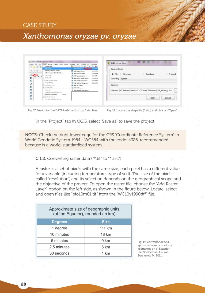
C1.1. Opening a shapefile in QGIS:
A shapefile has (at least) three files with the same name but with a different extension. The file with the SHP (“*.shp”) extension is the main file and includes spatial features.
Open the QGIS with the short option: add vector layer (left margin) or the “Layer” tab, as shown in the below figure:
C.1.2. Converting raster data (“*.tif” to “*.asc”):
A raster is a set of pixels with the same size; each pixel has a different value for a variable (including temperature, type of soil). The size of the pixel is called “resolution”, and its selection depends on the geographical scope and the objective of the project. To open the raster file, choose the “Add Raster Layer” option on the left side, as shown in the figure below. Locate, select and open files like “bio10m01.tif” from the “WC10y1990tiff” file.
Fig. 17. Search for the DATA folder and unzip *.shp files. Fig. 18. Locate the shapefile (*.shp) and click on “Open”.
In the “Project” tab in QGIS, select “Save as” to save the project.
NOTE: Check the right lower edge for the CRS “Coordinate Reference System” in World Geodetic System 1984 - WGS84 with the code: 4326, recommended because is a world-standardized system.
Fig. 19. Correspondencia aproximada entre grados y kilómetros en el Ecuador (de: Sheldeman X. & van Zonneveld M. 2011). Approximate size of geographic units
(at the Equator), rounded (in km)
Degrees 1 degree 10 minutes 5 minutes 2.5 minutes 30 seconds Size 111 km 18 km 9 km 5 km 1 km
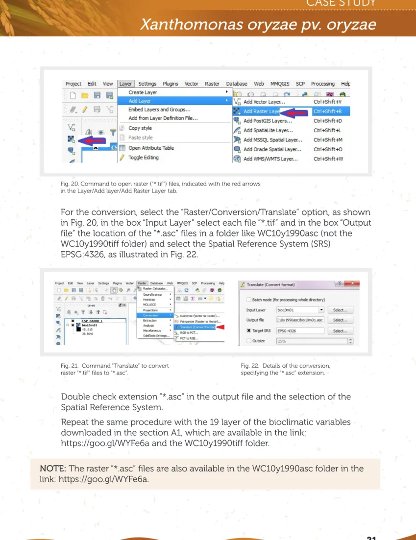
For the conversion, select the “Raster/Conversion/Translate” option, as shown in Fig. 20, in the box “Input Layer” select each file “*.tif” and in the box “Output file” the location of the “*.asc” files in a folder like WC10y1990asc (not the WC10y1990tiff folder) and select the Spatial Reference System (SRS) EPSG:4326, as illustrated in Fig. 22.
Fig. 20. Command to open raster (“*.tif”) files, indicated with the red arrows in the Layer/Add layer/Add Raster Layer tab.
Fig. 21. Command “Translate” to convert raster “*.tif” files to “*.asc”.
Fig. 22. Details of the conversion, specifying the “*.asc” extension.
Double check extension “*.asc” in the output file and the selection of the Spatial Reference System.
Repeat the same procedure with the 19 layer of the bioclimatic variables downloaded in the section A1, which are available in the link:
https://goo.gl/WYFe6a and the WC10y1990tiff folder.
NOTE: The raster “*.asc” files are also available in the WC10y1990asc folder in the link: https://goo.gl/WYFe6a.
C2. Using MaxEnt for the modeling.
To open the MaxEnt software, click on the “maxent.jar” file. Then open the “Settings” option, select “Basic” and include the standard option and the box “Random test percentage” write 25 for an additional software test with 25% of the samples. Then close the window.
In the main screen, in the samples option, select the “*.csv” (“Comma
separated values” not “*.xls”) file with the geo-referenced pest data. This was discussed in section A3.
Next, select "Auto features", "Create response curves", "Make pictures of predictions", "Do jackknife to measure variable importance", "Logistic format" and "asc file type", and select a folder for the output of the files, thus ordering a complete modeling, with figures like “Do jackknife” that visually describe the contribution of each bioclimatic variable to the final model. In the other part with the environmental layers option, choose the folder with the
converted variables to the “*. asc” format, i.e. a raster file like the one described in section A1.
For practical purposes, record warning messages like “Unused field” or “Missing environmental data” and click “Ok”.
Fig. 23. In “Settings” and “Basic”, include the standard options, as illustrated here.
Fig. 24. Main screen where geo-referenced data and bioclimatic variables are included in “*.asc” format.
The results of the environmental modeling are available in the
Xoryzaeoryzae.html file, which can be opened with any web browser. The raster file of the map is available in the Xoryzaeoryzae.asc file, as illustrated in the figure below.
C3. Open a map in geographical coordinates, creating a 100 km reference grid, and a centroid in each grid.
Develop a grid with a reference size of 100 Km or 0.9 decimal degrees, based on the equivalences of grades and kilometers from Sheldeman X. & van Zonneveld M. 2011, shown in the Fig. 19.
First, open a shape vector layer from COSIPLAN (http://www.sig.cosiplan.unasursg.org/node/15). Fig. 25. Record messages like: “Unused field”
o “Missing environmental data”.
Fig. 26. After checking the repetition of messages, you can select the “Suppress similar visual warnings” option.
Fig. 27. File with the results of the MaxEnt modeling.
Fig. 28. Opening the “*.html” file with the modeling. The “*.asc” file is a raster, as those described in section A1.
Fig. 29. Open a reference vector layer with the “*.shp” extension.
Fig. 30. Find the “Create Grid” function in the “Processing toolbox” (see the note below) and click it.
NOTE: If the Processing toolbox is not available, please select it in tab “View”, “Panels” and then “Processing toolbox”.
In the “Grid type” choose the “Rectangle (polygon)” option in the “Grid extent” choose “select extent on canvas” dragging the mouse on the map to create the grid. Complete “Vertical spacing” and “Horizontal spacing” with the 0.9 data. Check that EPSG 4326 – WGS84 is in “Grid CRS” and provide a route to save the grid file. Finally, click on “Run in Background” as illustrated in the figure below.
Fig. 31. Details included in the “Create grid” function.
Fig. 32. This is the grid file in the “Layers” panel. To make it transparent, select "Properties" with the right button.
NOTE: If the Processing toolbox is not available, please select it in tab “View”, “Panels” and then “Processing toolbox”.
In the “Layers” panel, you can change the grid file appearance and its location in the map with a right click on its name. To make it transparent, select “Options”, “Style”, “Single symbol”, “Fill”, “Simple fill”, and in “Fill style” select “No Brush”. Front or background movement on the map is commanded with a change in file position in the “Layers” panel.
Fig. 33. To make the grid transparent, select “Single symbol”, “Fill Style”, then “No brush”.
Fig. 34. To obtain centroids in each grid, look for the “Centroids” function (“Vector geometry” set) in “Processing Toolbox”.
NOTE: If the Processing toolbox is not available, please select it in tab “View”, “Panels” and then “Processing toolbox”.
Using this vector “*.shp” file of centroids, you can extract values from the modeling.
Fig. 35. Details in of the use of the “Centroids” function (“Vector geometry”).
Fig. 36. Results of the “Centroids” functions.
C4. Integrating information with QGIS
C4.1. Development a vector shapefile with the crop production information in the geo administrative geopolitical units of each co Develop a vector shapefile with crop production information in the administrative geopolitical units of each country:
First, open the file for the second level administrative geopolitical unit "CSP_FA001_P.shp" downloaded in section A2. Then with the right click on the file, select “Open attribute table” and “Toggle edition tool” by clicking on the pencil in the top left corner of the screen.
Fig. 37. Open the “CSP_FA001_P.shp” shapefile downloaded in section A2 and with a right click on the “Open attribute table” option”.
Fig. 38. Select the “Conmutar edición” with the pencil in the top left corner of the screen.
The vector file “CSP_FA001_P.shp” can include an additional column, where you can record the host area or a host risk index value like 0, 1 or 2 (2 as the
maximum value). The host area can be also a “Whole number (Integer)” having as many digits as the largest production area record. Both files are available in the https://goo.gl/WYFe6a folder.
Fig. 39. With the “New field” option you can include a column with the host area or a host risk index 0, 1 or 2; where 2 is the maximum value.
Fig. 40. Select the name, the “Whole number (Integer)” type, the “Length” of 1 and a click “Ok”.
C4.2. Converting a vector shapefile in a raster.
In order to integrate the host risk index, first convert the vector “*.shp” file to raster with a function in the tap “Raster”, “Conversions” and then “Rasterize (vector to raster)”. To do this, use the column with the host risk index for the value of the raster. The illustration of this function is shown in the figure below.
For a better view of model raster values, with a right click on the layer, open the “Properties” then “Style”, “Singleband pseudocolor” with the “Spectral” option. Include the modification of the label as HIGH, MEDIUM or LOW, as illustrated in the figure below.
Fig. 41. With the “Rasterize” function, convert the “CSP_FA001_P.shp” file using the host risk index as a value.
Fig. 42. For a better presentation of the bioclimatic risk model, change the properties with a right click on the layer.
C4.3. Reclassifying the raster of the model for its integration. Similarly to the host risk index, index 0, 1 or 2 is required in the environmental modeling. For this purpose, use the “Reclassify values
(simple)” function from SAGA (System for Automated Geoscientific Analysis) in the “Processing toolbox” on the right side of QGIS. In the function, select the “Fixed Table 3x3” option with the values 0, 1 or 2. These details are illustrated in the figures below.
Fig. 43. Location of the “Reclassify values (simple)” function in SAGA.
Fig. 44. Details of the “Reclassify values” function and the “Fix table 3x3”.
Moreover, it is possible to integrate the environmental risk with the host risk index or others with the “Raster calculator” function, which develops math between raster layers. With this tool, you can also integrate information on land cover or Normalized Vegetation Index (NDVI), which are raster files too. When raster layers are multiplied, the grids with a lower value are integrated with the zero (0) value, while higher categories are integrated with
maximum values, as shown in Table 3.
Table 3. Integrating raster files with the reclassification of the value in the grid and the multiplication function in the “Raster calculator”.
RASTER
INTEGRATION LOW INDEX B = 0 MEDIUM INDEXB = 1 HIGH INDEX B = 2 LOW INDEX
A = 0 LOW = 0 LOW = 0 LOW = 0 MEDIUM INDEX
A = 1 LOW = 0 MEDIUM = 1 MEDIUM = 2 HIGH INDEX
A = 2 LOW = 0 MEDIUM = 2 HIGH = 4
C4.4. Obtaining risk values with a vector shapefile
Open the centroid layer developed in section C3 to extract risk values to a vector (point) layer.
To include geographical coordinates, make a right click on the vector file and select “Open attributes table”. Then use the “Field calculator” as shown with the red arrow in the figure below and the “Geometry” option selecting $x for the field “longitude” and $y for the field “latitude”. It is important to check that the format of the field is “Decimal number (real)” and with 5 decimals of precision.
The figure below illustrates the use and results of the “Raster calculator” function:
Fig. 45. Details in the “Raster calculator” function for the integration of raster layers.
Fig. 46. Regional Risk map. Higher risk in red, medium risk in yellow and lower risk in light blue. Scale 1:45,000,000.
Fig. 47. With a right click on the vector shapefile, open the “Attributes table” and the “Field calculator”, as indicated with the red arrow.
Fig. 48. Create a field called “longitude” as “Decimal number (real) with 5 decimals and the “Geometry” function, then “$x” and similarly with “$y” for the “latitude”.
In the “Processing toolbox” on the right side, find the “v.sample” function and obtain raster values from the results of sections C2 or C4.3, as illustrated in the figures below.
Fig. 49. Sampling risk values with a vector shapefile in a new file “Sampled” in a new route for the file.
Fig. 50. The developed shapefile has points and values that can be graphically shown, changing layer properties.
This layer “Sampled” can be integrated with another vector shapefile, like the 100 km grid that created the centroids. For this, find the “Join attributes by location” function in the “Processing toolbox”. Select the “Sampled” layers and the “Grid” shapefile and save it, as illustrated in the figure below.
Fig. 51. Find the “Join attributes by location” function in order to integrate vector shapefiles.
Fig. 52. Select the layers to integrate with the “intercept” option and name this integrated layer.
This integrated information can be shown in a map, selecting with a right click the “Layer properties”, “Style” and “Categorize” in reference to the values of the modeling, as shown in the figures below.
It is also feasible to integrate other geo-referenced information, like the river layer “CSP_BH140_L.shp”, available in https://goo.gl/WYFe6a using the
“Intersection” function in the “Vector” tab and “Geoprocessing tools” group.
The vector shapefile resulting layer contains origin and modeled risk information. This information can be exported with the right click on the layer, as illustrated in the figures below:
Fig. 53. With the “Layer properties” function you can change the style display of the 100 km grid for risk value (high risk in red, medium risk in yellow and low risk in light blue).
Fig. 54. With the tool “Intersection”, located in the “Vector” tab, “Geoprocessing tools”, you can integrate vector shapefile information from the river layers.
Fig. 55. To collect the information in another format, you can select the layer with a right click and choose “Save as”.
Fig. 56. Save the information in CSV (“Comma separated values”) format, which can be opened in Microsoft Excel.
In Microsoft Excel, the NPPO can assess the risk parameters in based on expert criteria. The figure below provides an example.
Fig. 57. Raster risk value and the identification ID of each generated grid.
NOTE: All this case study information is available in the
cXanthomonasoryzaeoryzae folder in the link: https://goo.gl/WYFe6a.
NOTE: The QGIS generated map, “Bdorsalis.qgs”, is available in the “QBdorsalis” folder in the link: https://goo.gl/WYFe6a. To use it, download the “QBdorsalis” folder containing all the involved layers.
References
Costa P., Holtz V. 2011. Impacto das mudancas climáticas globais sobre a distribuicao geográfica da soja Brs valiosa RR no Brasil central. Anais do IX Seminário de Iniciação Científica, VI Jornada de Pesquisa e Pós-Graduação e Semana Nacional de Ciência e Tecnologia. Universidad Estadual de Goias. Available on January, 2018.
EPPO, 2003. Data Sheets on Quarantine Pests. Xanthomonas oryzae. European and Mediterranean Plant Protection Organization (EPPO), P Scott, CAB International. Available on October 27, 2017, at:
https://www.eppo.int/QUARANTINE/data_sheets/bacteria/XANTOR_ds.pdf
EPPO, 2017. EPPO Global Database: Xanthomonas oryzae pv. oryzae. Available on October 27, 2017, at: https://gd.eppo.int/taxon/XANTOR/photos
Morales N., Fernandez I., Baca-Gonzales V. 2017. MaxEnt's parameter configuration and small samples: are we paying attention to recommendations? A systematic review. PeerJ 5:e3093; DOI 10.7717/peerj.3093. Available on October 27, 2017, at: https://peerj.com/articles/3093/
Purdue University. 2017. Bacterial blight - Xanthomonas oryzae pv. oryzae. Available on October 27, 2017, at:
http://pest.ceris.purdue.edu/services/approvedmethods/sheet.php?v=681 http://download.ceris.purdue.edu/file/3055