Contribution to the cerebral forward model by depth electric stimulation and SEEG measurements : application in epilepsy

HAL Id: tel-00919480

https://tel.archives-ouvertes.fr/tel-00919480

HAL is a multi-disciplinary open access archive for the deposit and dissemination of sci-entific research documents, whether they are pub-lished or not. The documents may come from

L’archive ouverte pluridisciplinaire HAL, est destinée au dépôt et à la diffusion de documents scientifiques de niveau recherche, publiés ou non, émanant des établissements d’enseignement et de

application in epilepsy

Janis Hofmanis

To cite this version:

Janis Hofmanis. Contribution to the cerebral forward model by depth electric stimulation and SEEG measurements : application in epilepsy. Signal and Image processing. Université de Lorraine, 2013. English. �tel-00919480�

´

Ecole doctorale IAEM Lorraine

Universit´e de Lorraine

Contribution au mod`

ele direct c´

er´

ebral par stimulation

´

electrique de profondeur et mesures SEEG : application

`

a l’´

epilepsie (Contribution to the cerebral forward model

by depth electric stimulation and SEEG measurements :

application in epilepsy)

TH`

ESE

pr´esent´ee et soutenue publiquement le 20 Novembre 2013

pour l’obtention du

Doctorat de l’Universit´

e de Lorraine

Sp´ecialit´e Automatique, Traitement du Signal et des Images, G´enie informatique

par

J¯

anis HOFMANIS

Composition du jury

Rapporteurs : Ali MOHAMMAD-DJAFARI Sup´elec, CNRS UMR 8506, Univ Paris Sud 11

Michael WIBRAL Brain Imaging Center, Frankfurt J.W. Goethe University

Examinateurs : Maureen CLERC INRIA Sophia Antipolis Louis MAILLARD CRAN, CNRS UMR 7039 Val´erie LOUIS-DORR CRAN, CNRS UMR 7039 Olivier CASPARY CRAN, CNRS UMR 7039

R´esum´e

La thérapie de l’épilepsie par résection partielle exige l’identification des structures cérébrales qui sont impliquées dans la genèse des crises d’épilepsie focales. Plusieurs modalités telles que l’IRM, le PET SCAN, la sémiologie de la crise et l’électrophysiologie sont exploitées par les experts pour contribuer à la localisation de la zone épileptogène. L’EEG du scalp est la modalité qui pro-cure la résolution temporelle à l’échelle des processus électrophysiologiques étudiés. Cependant du fait du positionnement des capteurs sur le scalp, sa résolution spatiale et, plus précisément, de profondeur est très médiocre. Dans certain cas (épilepsies pharmaco-résistantes), et pour palier à cette déficience spatiale, il est possible d’avoir recours à la SEEG. La SEEG permet des mesures électrophysiologiques intracérébrales : la résolution spatiale et donc anatomique est excellente dans l’axe de la microélectrode. La définition de la zone épileptogène, comme celle proposée par Talairach et Bancaud, est une définition électro-clinique basée sur les résultats d’enregistrements de SEEG intracérébraux. Elle tient compte non seulement de la localisation anatomique de la dé-charge épileptique partielle, mais également de l’évolution dynamique de cette dédé-charge, c’est à dire les réseaux neurologiques actifs durant la période intercritique-critique et des symptômes cliniques. Récemment, il a été proposé une technique de diagnostic complémentaire de locali-sation de la zone epileptogénique employant la stimulation electrique cérébrale de profondeur (Deep Brain Stimulation). Cette source exogène peut activer les réseaux épileptiques et produire une réaction électrophysiologique telle qu’une crise d’épilepsie. Elle permet également de mettre en exergue les zones fonctionnelles cognitives. Cette source exogène est parfaitement définie spa-tialement et temporellement. Ainsi, la stimulation, couplée aux mesures SEEG, contribue à la modélisation de la propagation électrique cérébrale et, par voie de conséquence, à la compréhen-sion du processus épileptique De plus, ce travail sur le modèle de propagation directe apporte une aide à la résolution du problème inverse et donc à la localisation de sources. Les différentes tâches accomplies au cours de cette thèse sont les suivantes :

– Création d’une base de données réelles à partir de 3000 stimulations et mesures SEEG pour 42 patients explorés ;

– Extraction par séparation des signaux de propagation de la stimulation électrique (DBS) des mesures multidimensionnelles SEEG : 5 méthodes ont été développées ou adaptées et ont été validées au cours d’une première phase en simulation puis sur des signaux réels SEEG dans une seconde phase.

– Localisation des électrodes de SEEG dans le repère anatomique de l’IRM et du CT Scanner en y ajoutant une étape de segmentation de la matière grise et blanche, du liquide céphalo-rachidien et de l’os.

– Discussion sur de nombreux modèles de propagation réalistes ou non réalistes proposés dans la littérature, à la fois sur le plan du raffinement du modèle mais également sur les implantations numériques possibles : modèles de milieu, sphériques et réalistes infinis ba-sés sur MRI et CT du patient.

– Comparaison entre les résultats générés par les modèles de sources et de milieux et les données obtenues après séparation de la stimulation électrique in vivo chez l’homme. – Validation des modèles de tête FEM en intégrant les conductivités des milieux (CSF), gris

et blancs céphalo-rachidiens et perspectives envisagées.

Abstract

The study of epilepsy requires the identification of cerebral structures which are involved in generation of seizures and connexion processes. Several methods of clinical investigation con-tributed to these studies : imaging (PET, MRI), electrophysiology (EEG, SEEG, MEG). The EEG provides a temporal resolution enough to analyze these processes. However, the localization of deep sources and their dynamical properties are difficult to understand. SEEG is a modality of intracerebral electrophysiological and anatomical high temporal resolution reserved for some dif-ficult cases of pre-surgical diagnosis : drug-resistant epilepsy. The definition of the epileptogenic zone, as proposed by Talairach and Bancaud is an electro-clinical definition based on the results of intracerebral SEEG recordings. It takes into account not only the anatomical localization of par-tial epileptic discharge, but also the dynamic evolution of this discharge (active neural networks at the time of seizure) and clinical symptoms. Recently, a novel diagnostic technique allows an accurate localization of the epileptogenic zone using Depth Brain Stimulation (DBS). This exoge-nous source can activate the epileptic networks and generate an electrophysiological reaction. Therefore, coupling DBS with SEEG measurements is very advantageous : firstly, to contribute to the modeling and understanding of the (epileptic) brain and to help the diagnosis, secondly, to access the estimation of head model as an electrical conductor (conductive properties of tissues). In addition, supplementary information about head model improves the solution to the inverse problem (source localization methods) used in many applications in EEG and SEEG. The inverse solution requires repeated computation of the forward problem, i.e. the simulation of EEG and SEEG fields for a given dipolar source in the brain using a volume-conduction model of the head. As for DBS, the location of source is well defined. Therefore, in this thesis, we search for the best head model for the forward problem from real synchronous measurements of EEG and SEEG with DBS in several patients. So, the work of the thesis breaks up into different parts for which we need to accomplish the following tasks :

– Creation of database : ≈ 3000 DBS measurements for 42 patients ;

– Extraction of DBS signal from SEEG and EEG measurements using multidimensional anal-ysis : 5 methods have been developed or adapted and validate first in a simulation study and, secondly, in a real SEEG application ;

– Localization of SEEG electrodes in MR and CT images, including segmentation of brain matter.

– SEEG forward modeling using infinite medium, spherical and realistic models based on MRI and CT of the patient ;

– Comparison between different head models and validation with real in vivo DBS measure-ments.

– Validation of realistic 5-compartment FEM head models by incorporating the conductivities of cerebrospinal fluid (CSF), gray and white matters.

Contents

List of Figures v

List of Tables xv

1 Introduction 1

1.1 The Brain . . . 1

1.2 Bioelectricity of the brain . . . 4

1.2.1 Model of a Neuron . . . 6

1.2.2 Main brain rhythms . . . 7

1.2.3 Bioelectrical fields . . . 9

1.3 Epilepsy . . . 12

1.3.1 Seizure of epilepsy . . . 12

1.3.2 Epilepsy treatment . . . 13

1.3.3 The temporal lobe epilepsy . . . 14

1.4 The multi-modalities for epilepsy diagnosis . . . 15

1.4.1 Non-invasive methods . . . 15

1.4.2 Invasive methods . . . 18

1.5 EEG and SEEG measurements . . . 21

1.5.1 The electrical stimulation . . . 21

1.5.1.1 Stimulation and networks mechanism in epilepsy . . . 24

1.5.1.2 The amygdala-hippocampal stimulation . . . 24

1.6 Objectives of the thesis . . . 25

2 Multidimensional decomposition. Application to DBS separation in SEEG/EEG 27 2.1 Introduction . . . 27

2.2.1 Filtering approaches . . . 30

2.2.1.1 Savitzky-Golay Filter (SGF) . . . 30

2.2.1.2 Singular Spectrum Analysis (SSA) . . . 32

2.2.1.3 Empirical Mode Decomposition (EMD) . . . 34

2.2.1.4 Fast Intrinsic Mode Decomposition (IMD) . . . 37

2.2.2 Multidimensional analysis . . . 40

2.2.2.1 Filtering-GEVD approach . . . 41

2.2.2.2 Multi-channel SSA (MSSA) . . . 42

2.2.2.3 Multivariate EMD (MEMD) . . . 43

2.2.2.4 Blind Source Separation (BSS) . . . 43

2.3 (S)EEG data analysis using presented methods: examples and discussion . . . 45

2.3.1 Filtration and decomposition methods (mono-channel) . . . 46

2.3.2 Multichannel separation methods . . . 50

2.4 DBS source extraction from SEEG measurements . . . 56

2.4.1 DBS-SEEG acquisition . . . 57

2.4.2 Discussion of the DBS model . . . 60

2.5 Simulations and real datasets . . . 61

2.5.1 Synthetic datasets . . . 61

2.5.2 Real datasets . . . 63

2.6 Experiments and Results . . . 64

2.6.1 Parameters selection . . . 65

2.6.2 Estimation of performance . . . 65

2.6.3 Simulated SEEG data . . . 66

2.6.4 Real SEEG analysis . . . 71

2.7 Conclusion . . . 76

3 Localization of SEEG electrodes 77 3.1 Introduction and motivation of study . . . 77

3.2 Image Acquisition . . . 79

3.3 Registration . . . 79

3.3.1 Mutual information . . . 81

3.3.2 Optimization . . . 83

3.4 Matter segmentation . . . 84

CONTENTS

3.4.2 Non-brain tissue segmentation using CT . . . 87

3.4.2.1 Detailed algorithm . . . 87

3.4.3 Summary of segmentation process for 5 matters . . . 88

3.5 Electrode localization . . . 94

3.5.1 Skull Stripping . . . 95

3.5.2 Correlation of the pattern . . . 95

3.5.3 Identification of the Multicaptor . . . 95

3.5.4 Optimization of 3D localization . . . 97

3.5.5 Localization results and conclusion . . . 98

4 Forward modeling in vivo using DBS source 101 4.1 Physical and mathematical formulation of forward problem . . . 102

4.1.1 Notations . . . 102

4.1.2 Maxwell’s equations and quasi-static approximation . . . 103

4.1.3 Primary and secondary currents . . . 105

4.1.4 Final electric potential equation . . . 105

4.2 Infinite homogeneous medium . . . 106

4.3 Primary currents . . . 107

4.4 Boundary conditions . . . 108

4.5 Spherical models . . . 110

4.5.1 Single sphere method . . . 110

4.5.2 Multi-sphere method . . . 111

4.6 Realistic head models . . . 112

4.6.1 BEM . . . 113

4.6.2 FEM . . . 116

4.6.2.1 Linear shape functions . . . 119

4.6.2.2 Solving Linear equation system . . . 123

4.6.3 Meshing . . . 123

4.7 Summary and implementation of methods . . . 126

5 Validation and results: Forward models using real intracerebral DBS measurements 129

5.1 DBS source approximation models in FEM . . . 130

5.1.1 Error criterion for forward models accuracy . . . 131

5.1.2 Dipole and Source-Sink . . . 132

5.2 Sensitivity analysis of (S)EEG froward models . . . 134

5.2.1 Infinite Homogenous medium (IHM) . . . 135

5.2.2 Spherical models . . . 136

5.2.3 Realistic models . . . 138

5.2.3.1 BEM . . . 140

5.2.3.2 FEM . . . 144

5.2.3.3 One compartment BEM/FEM . . . 146

5.2.4 Performance and summary of applied methods . . . 146

5.3 Validation of forward models in real deep brain stimulation (DBS) measurements . . 150

5.3.1 Propagation data extraction . . . 151

5.3.2 Configuration of multi-electrode and stimulation dipole . . . 152

5.3.3 Results and discussion . . . 152

5.4 Influence of the CSF/Gray/White matter conductivity ratio in SEEG/EEG . . . 161

5.4.1 Optimization of CSF/Gray/White conductivities . . . 171

5.5 Conclusion . . . 173

6 Conclusion and Perspectives 175 6.1 Summary of the thesis . . . 175

6.2 Discussion and Perspectives . . . 177

6.3 Conclusion . . . 179

List of Figures

1.1 Two hemispheres of brain. . . 3

1.2 External view of brain with four lobes (temporal, frontal, occipital, and parietal) (191). 3 1.3 Diagram of a neuron (191). . . 4

1.4 Synapse structure (from

http://www.columbia.edu

1.5 Activation of a pyramidal cell creating the dipole field. . . 10

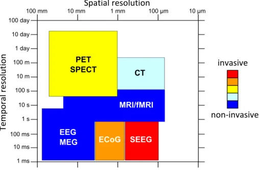
1.6 Spatial and temporal resolutions of the different brain imaging techniques (PET: Positron Emission Tomography, SPECT: Single-Photon Emission Computed Tomog-raphy, CT-scan: Computed Tomography scan, MRI: Magnetic Resonance Imaging, fMRI: functional MRI, EEG: ElectroEncephaloGraphy, MEG: MagnetoEncephaloGra-phy, ECoG: ElectroCorticoGraMagnetoEncephaloGra-phy, SEEG: Stereo-EEG) (5) . . . 18

1.7 SEEG electrodes. . . 19

1.8 ECoG electrode grid. . . 20

1.9 Implantation of SEEG electrodes. . . 20

1.10 EEG recording (Common reference montage). . . 22

1.11 Deep brain stimulation device. . . 23

2.1 Example of mixing model of sources. (a) three sources where first (from above) is 50 Hz of sin wave, second (middle) is 17 Hz sine wave and third is trend in triangular shape. (b) mixed sources with some random matrix A. The sampling frequency is 512 Hz. . . 29

2.2 SG Impulse Response: NSG= 5 , L = 20 . . . 31

2.3 Frequency Responses of SG and FIR Filters. Dotted blue line indicates -3 db level. . . 32

2.5 Examples of multidimensional signals (artificial and real). (a) artificial mixture of sources presented 2.1(a) on 6 channel measurements. (b) example of real SEEG measurements during DBS on 11 electrodes (DBS starting at 1.2 seconds; during 5 seconds). . . 46 2.6 Examples of DBS artifact filtration using classical filtering (9th_{measurement in figure}

2.5(b)). Signal 1 represents residue (DBS artifact) and signal 2, a filtered signal (SEEG activity + baseline) after low pass filtering. (a) Median filter (window of 6 samples). (b) Savitzky-Golay filter (N = 5, L = 20). . . 47 2.7 IMFs after EMD and IMD of example signals seen in figure 2.5. (a) IMFs of artificial

signal (figure 2.5(a), 3rd _{measurement) after EMD. (b) IMFs of SEEG with DBS}

(fig-ure 2.5(b), 9th _{measurement) after EMD. (c) IMFs of artificial signal (figure 2.5(a),}

3rd _{measurement) after IMD. (d) IMFs of SEEG with DBS (figure 2.5(b), 9}th

mea-surement) after IMD. Sifting stopping criterion for EMD is SD < 0.3. IMD used with a linear interpolation and the number of sifting iterations fixed to 3. . . 48 2.8 SSA of example signals (see figure 2.5). (a) First 16 reprojected uncorrelated

compo-nents of artificial signal in figure 2.5(a) (3rd _{measurement) using SSA (L = 30). (b)}

All reprojected uncorrelated components of SEEG with DBS seen in figure 2.5(b) (9th

measurement) using SSA (L = 10). Amplitudes of all components are normalized (standard deviation equals to 1). . . 49 2.9 Signal to be decomposed with SSA. . . 50 2.10 SSA Decomposition (L=15). . . 51 2.11 SSA-GEVD of example signals (in figure 2.5. (a) Unmixed components of artificial

signal in figure 2.5(a) using SSA with L = 30 and retaining the triangle component. (b) Unmixed components of SEEG with DBS seen in figure 2.5(b) using SSA with

L = 10 and retaining the first component (trend). Amplitudes of all components are

normalized (standard deviation equals to 1). . . 52 2.12 Classical BSS methods of example signals (in figure 2.5). (a) Unmixed components of

artificial signal in figure 2.5(a) using FastICA. (b) Unmixed components of SEEG with DBS seen in figure 2.5(b) using FastICA. (c) Unmixed components of artificial signal in figure 2.5(a) using SOBIRO. (d) Unmixed components of SEEG with DBS seen in figure 2.5(b) using SOBIRO. Amplitudes of all components are normalized (standard deviation equals to 1). . . 53

LIST OF FIGURES

2.13 MSSA of example signals (see figure 2.5). (a) First 16 components of artificial signal in figure 2.5(a) using L = 30 (b) First 25 components of SEEG with DBS seen in figure 2.5(b) usingL = 10. Amplitudes of all components are normalized (standard

deviation equals to 1). . . 54

2.14 Eigenvalues of components extracted with MSSA algorithm. (a) First 16 eigenvalues for components seen in figure 2.13(a). (b) First 25 eigenvalues for components seen in figure 2.13(b). . . 54

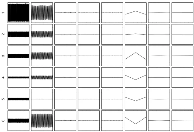
2.15 Resulting IMFs of MEMD for artificial sources. Extracted components (columns) for each measurement (rows) indicated by its number. . . 55

2.16 Resulting IMFs of MEMD for artificial sources. Extracted components (columns) for each measurement (rows) indicated by its number. . . 55

2.17 CT image of depth electrodes implantation scheme. . . 57

2.18 Theoretical DBS impulse. . . 58

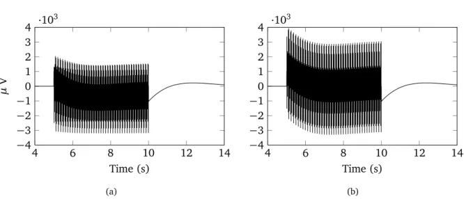
2.19 Measured DBS and its Fourier spectrum (SEEG). (a) DBS starting at 7th _{second and} during 5 seconds. (b) Spectrum of DBS after acquisition. . . 59

2.20 Modeled signal after different DBS acquisition steps (Micromed LTM 128). Blue line represents theoretical impulse (with amplitude of 1 V), black dots - digitization after first band bass filter, red dots - final acquired signal after FIR decimation (at sampling rate 512 Hz). . . 59

2.21 Simulated acquisition of a DBS on an electrode close to the stimulation site. . . 62

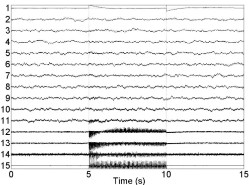
2.22 Example of 15 channels simulated DBS-SEEG with a noise level of 20 dB. . . 63

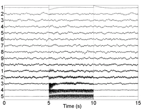
2.23 Real SEEG stimulation. Measurements of one multi-electrode. . . 64

2.24 SSA performance index over L. Red dot indicates the maximum performance. . . 66

2.25 Decomposed sources by SSA-GEVD using a dataset with 10 mixed SEEG sources and SNR = 20 dB. . . 67

2.26 Decomposed sources by SSA-GEVD using a dataset with mixed 15 SEEG sources and SNR = 20 dB. . . 68

2.27 Mean performance index for a different number of eliminated sources (n_{GEV D} and n_BSS) and different noise levels, in the case of 15 brain sources, for SSA-GEVD and FastICA. . . 69

2.28 Example of denoised mono-channel signal from a synthetic dataset of 15 SEEG sources without noise. Signal+Art: simulated mono-channel SEEG signal with trend and stimulation artifacts. Signal: simulated mono-channel SEEG signal without artifacts.

Following by denoised signals with the presented methods. . . 70

2.29 Mean performance index for each electrode at a 20 dB noise level using the presented methods. . . 71

2.30 Spectrograms of the 15 mixed SEEG sources estimated by SSA-GEVD (e) and FastICA (f) (data for 8th _{electrode). Noise level: SNR = 20 dB. (a) Data with artifacts, (b)} Stimulation artifact, (c) Trend artifact, (d) Data without artifacts. . . 72

2.31 Decomposed sources for real SEEG stimulation using SSA-GEVD. . . 73

2.32 Elimination of the stimulation and baseline artifacts from SEEG data with an epileptic activity during DBS (DBS ends at 3.1 s). . . 75

3.1 SEEG multi-captor . . . 79

3.2 Unregistered CT and MRI images used to guide the stereotactic surgery. . . 80

3.3 Unregistered CT and MRI images used to guide the stereotactic surgery. . . 82

3.4 Registered CT image using MRI as reference. Voxel size for both images (1 mm, 1 mm, 1 mm) . . . 85

3.5 Result of Freesurfer segmentation and reconstruction procedures: (a) labeled MRI axial cross-section after the Freesurfer matter segmentation procedure. Each color represents one intra-cerebral anatomical structure, in total about 40 structures. Im-age produced with 3D Slicer (http://slicer.org/), (b) gray (up) and white (down) matter surface reconstruction. . . 86

3.6 Histogram of 3D CT image. . . 88

3.7 Intensity threshold of a CT slice. (a) original slice without any thresholding; (b) background; (c) soft tissue, including skin, brain and some stereotaxic frame artifacts; (d) outer boundaries of skull and soft skull tissue; (e) hard skull tissue; (f) artifacts like electrodes, screws, wires and stereotaxic holding frame. . . 91

LIST OF FIGURES

3.8 Segmentation of skull performed on MRI (using Freesurfer/MNE) and CT (using au-thor’s segmentation algorithm). Boundaries are interpolated onto the image as black lines. (a) Slice of CT together with the outer skull boundary as acquired by author’s segmentation algorithm using the CT image. (b) Slice of CT together with the inner skull boundary as acquired by author’s segmentation algorithm using the CT image. (c) Slice of CT together with the outer skull boundary as acquired by Freesurfer/MNE using the MRI image. (d) Slice of CT together with the inner skull boundary as

ac-quired by Freesurfer/MNE using the MRI image. . . 92

3.9 Summary diagram of the segmentation process. . . 93

3.10 Labeled (segmented) image of 5 matters (scalp, skull, cerebrospinal fluid, gray, white). 94 3.11 CT image slices after skull stripping. . . 95

3.12 (a) blurred electrodes in slice of CT scan, (b) approximate pattern of electrode, (c) resulted image of correlation (maxima marked as red dots) . . . 96

3.13 Action diagram of the multicaptors’ registration. . . 96

3.14 The slice of correlation image with the line in direction of multicaptor. . . 98

3.15 Correlation intensity function along direction vector of the electrode. . . 99

3.16 Fitting of the sine wave (red) in correlation intensity function (blue). . . 99

3.17 Position of electrodes (black dots) as projected in CT image (rounding off decimal places to fit in CT voxel space). . . 100

4.1 Theoretical DBS impulse . . . 108

4.2 Interpretation of interface S_j between two domains with conductivities σ_j and σ_j+1. n(r) is the surface normal vector. . . 109

4.3 Diagram used to describe the potential at a point r within a single sphere model with a dipole at position r₀ and its momentum q. Volume of sphere Ω with external boundary S is with a radius R and a constant conductivity σ. rp= r − Kr0. . . 111

4.4 Diagram representing the concentric N-layered sphere model (multisphere) with radii R₁. . . R_N. The model consists of a measurement point r within a first sphere (consid-ered to be the approximation of a brain) with a dipole at position r₀and its momen-tum q. . . 112

4.5 Three closed surface meshes extracted from CT and MRI (see chapter (ref) ). a -approximation of brain or inner skull boundary, b - outer skull boundary, c - external head (skin) boundary. . . 114

4.6 Tetrahedron mesh of the head. Different colors indicate changes in element conduc-tivity. . . 117 4.7 Tetrahedron element ∆kwith local node points pkj, j = 1, . . . , 4 . . . 119

4.8 Residual of numerical solvers after each iteration until residual target (10−7_{) is reached.}

In legend: CG - Conjugate Gradient (without preconditioning), JP - CG with Jacobi Preconditionner, SOR - CG with Successive Overrelaxation. . . 124 4.9 Example of well and badly shaped mesh triangles. R radius of bounding circle, α

-minimal angle of the triangle ∆. (a) - well shaped triangle. α is close to optimal 60◦

angle. (b) - ill-shaped triangle. α is very small. . . 125 4.10 Flow diagram of FEM and BEM implementations. . . 127

5.1 Realistic electrode model (see image 3.1 from chapter 3). Radius of sphere - 80 mm, electrode distance from boundary of sphere - 17 mm. Electrode aligned on (with)

y-axis. Conductivity of sphere - 0.33 S/m . . . 130

5.2 The xy-slice (z=0) of simulated potential using realistic electrodes. The image shows interpolated potential on a regular grid. Potential outside conducting sphere is 0. Degrees of freedom (DoF) of model - 339360. . . 131 5.3 Potential and relative error of dipole and source-sink models compared to realistic

electrode model: (a) The x y-slice (z=0) of simulated potential using dipole as source model (DoF - 313429), (b) The xy-slice (z=0) of simulated potential using source-sink as source model (DoF - 311172), (c) RE % of dipole (V_appr) and realistic source (Vreal) model potentials and (d) RE % of source-sink (Vappr) and realistic source

(V_real) model potentials. . . 133 5.4 Final 3 compartment (scalp (gray), skull (red), intracranial space (yellow)) FEM

mesh with refined mesh around dipole position (green point). Radial and tangen-tial directions are indicated, respectively, by red and blue stick. . . 135 5.5 The reference solution of FEM. (a) radial dipole - parallel to z axis. (b) tangential

dipole perpendicular to z axis. For both models, conductivity is chosen as: scalp -0.33, skull - 0.01 and brain - 0.33 S/m. Dipole strength - 1 mA. . . 136 5.6 Simulated potential of IHM. (a) radial dipole - parallel to z axis. (b) tangential dipole

perpendicular to z axis. (c) and (d) - RE between IHM and reference FEM (from 5.5) both for radial and tangential dipoles. Conductivity of the infinite volume - 0.33. Dipole strength - 1 mA. . . 137

LIST OF FIGURES

5.7 Sphere fitting examples. (a) manually fitted sphere to upper boundary of the skull. Radius - 72 mm. (b) fitted sphere using Taubin’s method. Radius - 64 mm. . . 138 5.8 Simulated potential of Single sphere model (SSph) - automatic fitting. (a) radial

dipole - parallel to z axis. (b) tangential dipole perpendicular to z axis. (c) and (d) - RE between SSph and reference FEM (from 5.5) both for radial and tangential dipoles. Conductivity of the sphere volume - 0.33. Dipole strength - 1 mA. . . 139 5.9 Simulated potential of Single sphere model - manual fitting. (a) radial dipole -

par-allel to z axis. (b) tangential dipole perpendicular to z axis. (c) and (d) - RE between SSph and reference FEM (from 5.5) both for radial and tangential dipoles. Conduc-tivity of the sphere volume - 0.33. Dipole strength - 1 mA. . . 140 5.10 Simulated potential of Multi-Sphere model (3 sphere model). (a) tangential dipole

perpendicular to z axis. (b) - RE between MSph and reference FEM (from 5.5). Conductivities are chosen same as in the FEM model: outer sphere (scalp) - 0.33, middle sphere (skull) - 0.01 and inner sphere (brain) - 0.33 S/m. Dipole strength - 1 mA. . . 141 5.11 Simulated potential of Classical BEM approach. (a) radial dipole - parallel to z axis.

(b) tangential dipole perpendicular to z axis. (c) and (d) - RE between Classical BEM and reference FEM (from 5.5) both for radial and tangential dipoles. Conductivities are chosen same as in the FEM model: scalp - 0.33, skull - 0.01 and inner skull (brain plus cerebrospinal liquid) - 0.33 S/m. Dipole strength - 1 mA. . . 142 5.12 Simulated potential of IPA BEM. (a) radial dipole - parallel to z axis. (b) tangential

dipole perpendicular to z axis. (c) and (d) - RE between IPA BEM and reference FEM (from 5.5) both for radial and tangential dipoles. Conductivities are chosen same as in the FEM model: scalp - 0.33, skull - 0.01 and inner skull (brain plus cerebrospinal liquid) - 0.33 S/m. Dipole strength - 1 mA. . . 143 5.13 Simulated potential of IPA BEM. (a) radial dipole - parallel to z axis. (b) tangential

dipole perpendicular to z axis. (c) and (d) - RE between IPA BEM and reference FEM (from 5.5) both for radial and tangential dipoles. Conductivities are chosen same as in the FEM model: scalp - 0.33, skull - 0.01 and inner skull (brain plus cerebrospinal liquid) - 0.33 S/m. Dipole strength - 1 mA. . . 144

5.14 Simulated potential of low resolution FEM. (a) radial dipole - parallel to z axis. (b) tangential dipole perpendicular to z axis. (c) and (d) - RE between FEMlow and

reference FEM (from 5.5) both for radial and tangential dipoles. Conductivities: scalp - 0.33, skull - 0.01 and inner skull (brain plus cerebrospinal liquid) - 0.33 S/m. Dipole strength - 1 mA. . . 145 5.15 Relative errors of one compartment BEM/FEM. (a) and (b) - RE between BEMInt ra

and reference FEM for the radial and tangential dipoles respectively. (c) and (d)

-RE between FEMInt raand reference FEM for the radial and tangential dipoles

respec-tively. Conductivity of the volume - 0.33 S/m. Dipole strength - 1 mA. . . 147 5.16 Propagation coefficient extraction from DBS measurements. . . 152 5.17 Multi-electrode implantation scheme. . . 153 5.18 Forward models compared with extracted measurements of 6 electrodes for the

M’1-M’2 stimulation (see table 5.4).(a) - P’ (b) - B’ (c) - S’ (d) - X’ (e) - F’ (f) - L’. The information marker representing each model is given next to the figure (a). . . 155 5.19 Forward models compared with extracted measurements of 6 electrodes for the

C’1-C’2 stimulation (see table 5.4).(a) - P’ (b) - B’ (c) - S’ (d) - R’ (e) - F’ (f) - T’. The information marker representing each model is given next to the figure (a). . . 156 5.20 Forward models compared with extracted measurements of 5 electrodes for the

S’1-S’2 stimulation (see table 5.4).(a) - B’ (b) - C’ (c) - F’ (d) - L’ (e) - M’. The information marker representing each model is given next to the figure (a). . . 157 5.21 Forward models compared with extracted measurements of 6 electrodes for the

X’1-X’2 stimulation (see table 5.4).(a) - P’ (b) - B’ (c) - R’ (d) - S’ (e) - F’ (f) - T’. The information marker representing each model is given next to the figure (a). . . 158 5.22 Forward models compared with extracted measurements of 6 electrodes for the

L’1-L’2 stimulation (see table 5.4). (a) - T’, (b) - B’, (c) - R’, (d) - C’, (e) - F’, (f) - X’. The information marker representing each model is given next to the figure (a). . . 159 5.23 Forward models compared with extracted measurements of 6 electrodes for the

C’9-C’10 stimulation (see table 5.4).(a) - P’ (b) - R’ (c) - S’ (d) - F’ (e) - X’ (f) - M’. The information marker representing each model is given next to the figure (a). . . 160 5.24 5 compartment (scalp, skull, CSF, gray and white matter) FEM mesh with refined

LIST OF FIGURES

5.25 5 compartment FEM solution compared to 3 compartment reference FEM used in section 5.2. (a) - RE % of radial dipole, (b) RE % of tangential dipole. Conductivities of 5 volumes: scalp - 0.33 S/m, skull - 0.01 S/m, CSF - 0.5 S/m, gray matter - 0.3 S/m, white - 0.20 S/m. . . 163 5.26 5 compartment FEM models with different conductivities compared with extracted

measurements of 6 electrodes for the M’1-M’2 stimulation (see table 5.4).(a) - P’ (b) - B’ (c) - S’ (d) - X’ (e) - F’ (f) - L’. The information marker representing each model is given next to the figure (a). . . 165 5.27 5 compartment FEM models with different conductivities compared with extracted

measurements of 6 electrodes for the C’1C’2 stimulation (see table 5.4).(a) P’ (b) -B’ (c) - S’ (d) - R’ (e) - F’ (f) - T’. The information marker representing each model is given next to the figure (a). . . 166 5.28 5 compartment FEM models with different conductivities compared with extracted

measurements of 5 electrodes for the S’1S’2 stimulation (see table 5.4).(a) B’ (b) -C’ (c) - F’ (d) - L’ (e) - M’. The information marker representing each model is given next to the figure (a). . . 167 5.29 5 compartment FEM models with different conductivities compared with extracted

measurements of 6 electrodes for the X’1X’2 stimulation (see table 5.4).(a) P’ (b) -B’ (c) - R’ (d) - S’ (e) - F’ (f) - T’. The information marker representing each model is given next to the figure (a). . . 168 5.30 5 compartment FEM models with different conductivities compared with extracted

measurements of 6 electrodes for the L’1L’2 stimulation (see table 5.4). (a) T’, (b) -B’, (c) - R’, (d) - C’, (e) - F’, (f) - X’. The information marker representing each model is given next to the figure (a). . . 169 5.31 5 compartment FEM models with different conductivities compared with extracted

measurements of 6 electrodes for the C’9-C’10 stimulation (see table 5.4).(a) - P’ (b) - R’ (c) - S’ (d) - F’ (e) - X’ (f) - M’. The information marker representing each model is given next to the figure (a). . . 170

List of Tables

2.1 Empirical Mode Decomposition with sifting process . . . 35 2.2 Details of the EMD algorithm applied to the test signal. . . 35 2.3 Multivariate Empirical Mode Decomposition . . . 44 2.4 Comparison of filtering-GEVD, FastICA and SOBIRO algorithms using simulated data

with different levels of additive noise. Mean performance index and mean standard deviation in brackets for all 15 electrodes after 1000 trials. . . 69 2.5 Comparison of filtering-GEVD, FastICA and SOBIRO algorithms using real datasets

(1187 DBS multichannel recordings). Index of correlation and standard deviation in brackets for n fixed and calculated by the criterion. . . . 74

3.1 Powell’s optimization method for multi-variable functions. . . 84 3.2 Segmentation steps of the inner skull using CT. . . 89 3.3 Segmentation steps of the outer skull using CT. . . 90

4.1 Comparing the iterations and time of convergence for Conjugate Gradient solvers with and without preconditioning. Solving V for source-sink model with A of di-mensions 171018 × 171018,

cond

-conjugate gradient without preconditioning, JP - Jacobi preconditionner CG and SOR - Gauss-Seidel preconditionner CG. . . 124

5.1 Relative difference over x y slice for dipole and source-sink current models including and excluding saturation limits (under -5000 and over 5000 µV ) . . . 132 5.2 RDM% (RDM × 100) comparing reference FEM and other forward models for one

dipole position (two orientations - tangential and radial). Main value - RDM% in in-tracranial volume, value in parenthesis - RDM% for model containing volume space. NA - not applicable. . . 148

5.3 Performance time (in seconds) of different forward modeling aspects: Img to mesh - labeled image transformation to usable mesh; Building model - system matrix and load vector calculations; Solving for a dipole - calculating the potential of single dipole for 100 field points (electrodes). NN stands for Not Necessary or model does not need this procedure. . . 149 5.4 Detailed information on the chosen DBS for the patient. . . 153 5.5 RDM% (RDM × 100) of forward models and extracted DBS potential for 6

stimula-tions. In the last column, the total RDM% of all combined DBS is provided. . . 154 5.6 RDM% (RDM × 100) of 5 compartment FEM with different conductivity

combina-tions of CSF, gray and white matter. RDM% is given for 6 DBS and total of all DBS combined. . . 164 5.7 Optimized conductivities of CSF, gray and white matter respectively (scalp - 0.33 and

Chapter 1

Introduction

If the brain were so simple that we could understand it, then we’d be so simple that we couldn’t.

—Ian Stewart

The human brain is an eminently complex and still incompletely known system. One distin-guishes mainly two types of approach to describe it: the structural level and the functional level. In the first case, the brain is regarded as a number of interconnected biological structures. The level of these structures can vary from a large cerebral area to the single neuron. If it is described under the functional system, the brain is seen as a number of functions which interoperate between them: the study can be led at various scales, from the very complex cognitive function to the functional primi-tive. The two aspects are bound, of course, inasmuch as the anatomical level is the physical support of the functional level. The functional neuroimagery is the principal tool making it possible to study this connection between the functional process and the structure. However, this tool is imperfect. Initially, the spatial and temporal scales were not compatible with the study of temporal dynamic of the neuronal activity, or its precise spatial localization. In addition, it is not directly the neuronal activity which is observed with the techniques of neuroimagery, but some of its manifestations. In the objective of a modeling, this chapter aims to present the heterogeneous and incomplete knowl-edge on the brain which has been published in the literature from the anatomical and functional description.

1.1

The Brain

The brain acts as the origin of ordering not only for the thoughts, the memory, the perception of the world through the senses, but also for the muscles and gestures. It forms a central highly-strung

person component of the system as well as the cerebellum, the brain stem and the spinal-cord. Lo-cated in the brain-pan, the brain represents only 2 % of the total weight of the body but consumes 20 % of its energy, whether person is awake or asleep. Its volume is about 300 cm3_{, the cortical}

surface area reaching 2,200 cm2_{. Because of its folded structure, the apparent cortical surface area}

accounts for only 25 to 30 % of the totality of its surface. The thickness of the cortex varies from 1.5 to 4.5 millimeters according to the location. The cellular density differs according to the type of cortex: from 14,000 to 18,000 neurons/mm3 _{in the agranular cortex and from 40,000 to 100,000}

neurons/mm3 in the visual cortex. The number of neurons in the cerebral cortex is, according to the authors in (106), ranging from 109 _{to 10}11_{. Each pyramidal cell can receive between 10}4 _and

105_{synapses. The total amount of connections that the cortex could thus reach is 1 million billion.}

The arteries make it possible to feed the brain continuously with glucose and oxygen to provide for such energy needs, more especially as the brain is able to store only very little energy, for one very limited duration.

The human nervous system is subdivided anatomically into a Central Nervous System (CNS), including the brain and spinal-cord, and a peripheral nervous system, joining together the nerves which travel all over the body to cover all organs.

The brain contains two hemispheres (right and left - figure 1.1), and each is divided into four lobes (218) (see figure 1.2):

• the frontal lobe, located in the former part of the cerebral hemispheres (behind the face), contains the centrex responsible for voluntary driving coordination, as well as the centrex of thought, of memory and of the reasoning process;

• the temporal lobe, located on the side, on the level of the temple, contains the centrex of hearing, the language and the visual recognition of the objects;

• the occipital earlobe, located in the posterior part of the hemispheres, contains the structures for the vision;

• the parietal lobe, located in front of the occipital lobe, in the mid-sized part of the brain, contains the centre relating to the touch and the spatial guidance.

The peripheral gray substance of the cerebral hemispheres which presents complex convolutions constitutes the cerebral cortex of the brain.

1.1 The Brain

Figure 1.1: Two hemispheres of brain.

1.2

Bioelectricity of the brain

Neurons are the cells responsible for the transmission of information in the brain. They generate and transmit a signal called the flux nerve impulse. The full number of neurons in the human brain is estimated at approximately 100 billion. In figure 1.3, a typical neuron is shown what consists of:

• a cell body (or soma), which contains the cellular nucleus and cytoplasm which surrounds it, and which ensures the synthesis of the components necessary to the job functions of the neuron,

• a dendrite, which is the branched projections of a neuron (one speaks of dendritic tree), which act as receptors for the neuron by propagating the related electrical signals,

• an axon, which is a long prolongation playing a part of transmitter towards the other neurons.

• terminal buttons which are the small knobs at the end of an axon that release chemicals called neurotransmitters.

1.2 Bioelectricity of the brain

The junction between the axon terminal of a neuron and a dendrite or the soma of another neuron is called a synapse. It is a structure that enables a neuron (or nerve cell) to transmit electrical or chemical information to another system or cell (neural or otherwise like muscle for example). There exist chemical synapses, utilizing electric neurotransmitters, and synapses, for which the electrical signals are transmitted directly. A presynaptic element, an axon, and a postsynaptic element, for example a dendritic one, are in close apposition to the synapse but not in direct contact with it. The pre and postsynaptic membranes are separated by a gap called synaptic cleft (see figure 1.4). Chem-ical transmitters bridge this gap by diffusing from release sites on the presynaptic side to receptors on the postsynaptic side. According to their effect, one differentiates the exiting synapses and the inhibiting synapses.

Synaptic transmission begins when the action potential reaches the axon terminal. Chemical

synap-Action potential _presynaptic

membrane postsynaptic membrane synaptic cleft synaptic vesile neurotransimtters

Figure 1.4:Synapse structure (fromhttp://www.columbia.edu).

tic transmission involves the physical movement of ions, molecules, and membranes as part of the signaling event, as well as during recovery from a signaling event. These mechanistic constraints limit the time scale at which synaptic transmission can function and dynamically alter the ampli-tudes of synaptic responses in ways that depend on recent history: such dynamics can last from milliseconds to tens of seconds (111). To understand the input - output relationships of the neuron model, it is necessary to define the synaptic input, which may be modeled in two ways: as current synapses or conductance synapses. Synaptic background activity is invariably present in intracellu-lar recordings of neocortical neurons in vivo.

1.2.1

Model of a Neuron

Neurons are continuous, dynamical systems and neuron models must be able to describe smooth, continuous quantities such as graduated transmitter release and time average pulse intensity (99). The excitation of a neuron through a synapse involves the opening of the channels on the level of its membrane. The ionic composition being different inside and outside the cells, the opening of the channels generates a moving of particles charged in the intra and extracellular compartments. These currents known as primary currents are at the origin of EEG measurements. They are the post-synaptic currents generated in the dendrites of the cells that are collected on the scalp and intra electrodes.

The potentials of action being propagated along the axons of the nerve cells generate two cur-rents of opposite sense and thus a quadripolar electromagnetic field, which attenuates very quickly with depth. Those potentials are not detectable outside the skull (127). However, it has been shown that the action potential is detectible by microelecrode recordings but still unclear how much it is exposed to intracranial EEG with relatively large electrode surface area.

The primary or source currents then generate secondary currents called volume currents. In order to maintain the conservation of the energy, the formed threads of currents are closed after circulation in the whole volume of the head (77).

The compartmental models describe the neuron at the inner scale, through various compart-ments (axon, synapse, cellular body) and coupled with differential equations, allowing to build the neuron models and numerically predict the neural activity. Many papers have been published in the field of neuron modeling. The first plausible and probably most cited model is that of Hodgkin and Huxley (93). Most recent models describe the ion channels on the tree-like spatial structure of the neuronal cell, and integrate and fire models based the simple idea of accumulating synap-tic inputs and electric currents and when the neuron membrane reaches some threshold, the action potential or spike is relished. Integrate and fire principle have become widely approved neuron mod-els in studies of neural systems (27). Electrophysiologists generally prefer the biophysical modmod-els, familiar with the notion of ion channels that open and close (and hence, alter neuronal activity) de-pending on environmental conditions. These models are a nonlinear ordinary differential equations

1.2 Bioelectricity of the brain

system consisting of four equations describing the membrane potential, activation and inactivation of different ionic gating variables and it takes into account the conductance channels. Alan Lloyd Hodgkin and Andrew Huxley managed to explain the ionic mechanisms underlying the initiation and propagation of action potentials in the squid giant axon, and received the 1963 Nobel Prize in Physiology or Medicine for their work. Later, many studies were variations of their model, see Long and Guoliang Fang, 2011 for the review (129). In this paper, five different neuron models for possible use in spiking neural networks were evaluated. The neuron models have a wide range of possible biological plausibility and computational difficulty. While previous studies have suggested that very large time step sizes can be used, this results in solutions which do not converge to the same answer when the time step size is reduced. According to Burkit (26), in order to model in vivo neurons, it is necessary to take into account the apparently random times of arrival of the synaptic inputs. This way was initiated by Gerstein and Mandelbrot in 1964 with the diffusion approach using stochastic differential equations and the Ornstein Uhlenbeck process (205). Some authors (112, 119, 124, 192, 193, 204, 220) then explored this work and subsequently investigated the model using both stochastic differential equations and numerical techniques. However, if the study of the behavior of a single neuron is very interesting, it is quite as important to study the interaction of a population of neurons and networks. Then, in a larger scale, the dynamic neural electric fields can explain the brain functions or pathologies.

1.2.2

Main brain rhythms

In order to understand how the electrical signals of the brain are generated, it is necessary to try to model and understand how the activity of a population of neurons is organized both in time and in space, and which biophysical laws govern the generation of extracellular field potentials or magnetic fields (130). As we saw above, it is generally assumed that the neuronal events that cause the generation of electric and/or magnetic fields in a neural process consist of ionic currents that have mainly postsynaptic sources. For these fields to be measurable at a distance from the sources, it is important that the underlying neuronal currents are well organized both in space and time. According to Lopes Da Silva (130), at the macroscopic level, the activation of a set of neurons organized in parallel is capable of creating dipole layers. Important conditions that have to be satisfied for this to occur are the following:

• the neurons should be spatially organized with the dendrites aligned in parallel, forming palissades, and

• the synaptic activation of the neuronal population should occur in synchrony.

In the neocortex, the small volume corresponds to hypothetical cortical modules, for example mini or macro columns with mostly parallel organised layers of principal cells and numerous in-terneuron types (30). Brain regions with parallel arranged dendrites and afferents, such as cortical structures, give rise to large amplitude extracellular potentials, whereas subcortical nuclei with a less orderly spatial organization generate closed fields i.e. small-amplitude field events. A fundamental property of a neuronal network is the capacity of the neurons to work in synchrony. This depends essentially on the way the inputs are organized and on the network inter-connectivity. Thus, groups of neurons may work synchronously as a population due to mutual connections (130).

Network oscillations are attractive for cellular neurophysiologists interested in understanding network behavior in terms of the underlying biophysical mechanisms. Synchronous oscillations can be studied in detail using in vivo preparations. Therefore, for neurophysiologists and theorists alike, the study of synchronous rhythms is an excellent way to investigate how collective network dynam-ics emerges from the interplay between cellular biophysdynam-ics and synaptic circuits (214).

The visual and automatic studies of EEG play a very important part in the diagnosis of many cerebral electrophysiological disorders. The durations, amplitudes, forms and frequencies are thus fundamental components of the EEG (20) signal. The term rhythm is used when the waves have a homogeneous amplitude and also duration. In EEG, five rhythms (waves or activities) are distin-guished. Their wavebands cover the domain of frequency of the EEG. The first classification of the brain rhythms was introduced by the International Federation of Societies for Electroencephalogra-phy and Clinical NeuroElectroencephalogra-physiology in 1974 and it was driven by pragmatic clinical consideration.

These rhythms are: delta (δ), theta (θ), alpha (α), beta (β) and gamma (γ).

1. Rhythm δ (0,5–4 Hz): associated with deep sleep and probably present in a state of weakness. Its waves are very slow and generally have a great amplitude. It is current in young children aged less than one year and in this context constitutes the dominating rhythm.

2. Rhythm θ (4–8 Hz): appears during the sleep or the periods of time of concentration. Some work located a theta activity, induced by tasks of mental calculation, on the central line of the frontal lobe (142). This type of rhythm can also appear during meditation (92) and during the procedures of storage operation (180). It is frequent in children up to 13 years old but

1.2 Bioelectricity of the brain

the abundant presence of a theta or asymmetrical rhythm in the conscious adult is abnormal (211).

3. Rhythm α (8–13 Hz): with an amplitude between 30 and 50 µV, it appears mainly in the posterior areas (behind the vertex). Its distribution is bilateral and symmetrical and has a sinusoidal morphology; however, in some cases it can be presented in a form of sharp waves (178). Its appearance is supported by the closing of the eyes and by the relaxation therapy, it is thus attenuated by the increase in vigilance, with a tendency to disappear at the time of a mental activity and by the opening of the eyes.

4. Rhythm β (13–30 Hz): has a localization in the mid-sized areas of the two hemispheres in an asynchronous way. Its amplitude is lower than 30 µV and is usually masked by the rhythm

α. Beta rhythms are normal for an adult and is associated with the mental activities, such as

attention, problem-solving and the comprehension of the outside world. High contents of the

β rhythms can be observed in a state of panic.

5. Rhythm γ (>30 Hz): refers to the frequencies beyond 30 Hz. Its small amplitude and very uncommon presence make it hardly detectable in the EEG of surface area but accessible with intracranial EEG measurements. It could be associated with the synch between various cere-bral surfaces implied in the same functional network to associate the essential information with the execution of high-level tasks (209).

1.2.3

Bioelectrical fields

In brief, the ionic mechanism of the neurons can generate two types of electrical potentials:

• postsynaptic potential: in a junction of neuro-transmitters, an ionic exchange (Na+ and K+) is created by the permeability of the membrane and drives the formation of a membrane potential.

• action potential: if many postsynaptic potentials are generated at the same time, the mem-brane potential of the soma can locally reach a certain threshold which makes the neuron to

spike : some voltage-sensitive channels open, allowing positive ions to flow.

With those two types of potentials, all excitation or inhibition processes on the neural level can generate a small amount of electrical activity in the neuron which can be approximated by mathematical dipoles. In electrostatics, an electric dipole is the configuration obtained when two

charges, one negative and one positive, are coming close to each other along a certain axis. A dipole is defined by its position (where the charges are located), and its moment, a vector pointing from the negative to the positive charge and whose amplitude is given by the magnitude of the charges times the distance between them. An electric dipole creates an electromagnetic field as seen in image 1.5.

Figure 1.5:Activation of a pyramidal cell creating the dipole field.

Electric currents of the dipole spread to the surface of the head, traversing highly resistant skull compartment. An electrode at a certain point of the scalp can measure the potential field, it is the EEG scalp. The electrodes used on the EEG scalp are large and remote. They only detect summed activities of a large number of neurons (104_{) which are synchronously electrically active. The action}

potentials can be large in amplitude (70-110 mV) but they have a small time course (0,3 ms) (84). Their time course is larger (10-20 ms). This enables summed activity of neighboring neurons.

1.2 Bioelectricity of the brain

However, their amplitude is smaller (0,1-10 mV).

Thus, in order to view an electrical activity at the level of the scalp, one needs several hundreds of millions of synchronized neurons, between 107 and 108 according to Nunez (147). Moreover, it is necessary for all the cells to be laid out in parallel to each other and perpendicular to the surface area of the cortex, so that their activity is summed. As a result, for the potential to be viewable, the minimal cortical surface area is estimated to be at 6 cm2_.

EEG reflects the electrical activity of a subgroup of neurons, especially pyramidal neuron cells, where the apical dendrite is systematically oriented orthogonal to the brain surface. The pyramidal neurons are located mostly in the gray matter of the cortex. Certain types of neurons are not sys-tematically oriented orthogonal, so all the neuronal activity is not visible at the surface. The patches of synchronously polarized brain neurons must not only cover a considerable area but also need one dominant orientation to result in a far field at the scalp(206).

The passive transmission of electric fields through tissue from an underlying electrical current gen-erator is known as volume conduction. The macroscopic Maxwell equations are an (incomplete) system of partial differential equations, which describes the electromagnetic fields in a conducting, polarizable and magnetizable medium. Although volume conduction follows Maxwell’s equations, for the low frequency activity characteristic of the EEG in a matter, it can be efficiently simplified by neglecting the capacitive component of tissue impedance, as well as induction and the related electromagnetic propagation (154, 155, 195). To model the scalp potential, it is crucial to have a head model capable of describing the potential distribution on the scalp due to an intracranial current dipole.

In principle, the relation is described by differential equations (55, 147) which can only be solved nu-merically or for models approximating the head by different spheres of homogeneous and isotropic conductivities for scalp, skull, cerebrospinal fluid and brain matter. Each scalp electrode senses activity from each source with a specific relative attenuation coefficient depending on the geomet-rical configuration of the source and the location of the electrode relative to the source. For the dipole sources, the contribution of source activities to the electrode potential depends on electrode location, source location, orientation and the conduction properties of the volume conductor. The modeling of the electrical field in/on the volume conductor for a given source configuration, is called the forward problem or forward modeling. The counter procedure, where potential field values are use to locate a particular source is called the inverse problem or source localization.

1.3

Epilepsy

Epilepsy is a chronic neurologic affection characterized by the repetition of seizures caused by ab-normal electric discharges. The term seizure refers to a transient alteration of behavior due to abnormal, synchronized, and repetitive burst firing of neuronal populations in the central nervous system (CNS). Epilepsy is a syndrome of episodic brain dysfunction characterized by recurrent un-predictable spontaneous seizures. Partial seizures begin in a localized brain region, whereas gen-eralized seizures show widespread involvement of both hemispheres from the outset (187). The elements of definition of epilepsy given by Fisher in (62) are:

• History of at least one seizure

• Enduring alteration in the brain that increases the likelihood of future seizures

• Associated neurobiologic, cognitive, psychological, and social disturbances

In France, the prevalence of the epilepsy (i.e. the proportion of the population affected by this disease at one given moment) is estimated at approximately 0,5 %. Besides, anybody can undergo a single seizure in their lifetime (that can touch up to 5 % of the population). However, the diagnosis of epilepsy is reserved to the people suffering from repeated seizures.

1.3.1

Seizure of epilepsy

The definition of a seizure given by Fisher in (62) and proposed by the International League Against Epilepsy (ILAE) and the International Bureau for Epilepsy (IBE) is: An epileptic seizure is a transient occurrence of signs and/or symptoms due to abnormal excessive or synchronous neuronal activity in the brain. Epilepsy is a disorder of the brain characterized by an enduring predisposition to generate epileptic seizures and by the neurobiologic, cognitive, psychological, and social consequences of this condition. The definition of epilepsy requires the occurrence of at least one epileptic seizure.

The paroxysmal electrical activities produced during the seizures can either occur in a precise area in the cases of partial seizures or focal distances, or to be propagated in the group of neuron in the cases of generalized seizures. The partial epilepsies are most frequent type of epilepsy, that is to say 60 % of all cases. According to the origin of the epilepsy, the partial and generalized epilepsies can be classified in three types (52):

1.3 Epilepsy

• the idiopathic epilepsies, due to a real genetic predisposition, or at least a supposed one, inde-pendently of any brain injury,

• the cryptogenic epilepsies, which are expected to be symptomatic, but whose causes cannot be found by the current means of investigation. However, an epilepsy considered to be crypto-genic is likely to evolve into a symptomatic epilepsy because of the continual change in the means of browsing.

Given that the basic mechanism of neuronal excitability is the action potential, a hyperexcitable state can result from increased excitatory synaptic neurotransmission, decreased inhibitory neuro-transmission, an alteration in voltage-gated ion channels, or an alteration of intra- or extra-cellular ion concentrations in favor of membrane depolarization. A hyperexcitable state can also result when several synchronous subthreshold excitatory stimuli occur, allowing their temporal summation in the postsynaptic neurons (25).

1.3.2

Epilepsy treatment

To control the seizures, the drug treatments are often useful, but between 20 and 30 % of the patients suffering from epilepsy continue to have seizures despite the treatment (52). Such cases are referred to drug-resistant epilepsies. Among the temporal epilepsies which constitute the major part of partial epilepsies, at least 15 % are considered drug-resistant.

The goal of epilepsy evaluation in a clinical centers is firstly to clarify the diagnosis thanks to a recording video-EEG (electroencephalogram) prolonged to capture the epileptogenic events: are they really demonstrations epileptics or psychogenic seizure. If the epileptic diagnosis is confirmed, the distinction between generalized epilepsy and focal epilepsy allows to choose the drug treat-ment. In the focal and drug resistant epilepsies, a thorough assessment of imaging (MRI, PET) aims at locate the focus of the epileptic seizure (dysplasia) and its proximity with the cognitive processes (language, motricity, sensitivity, vision, memory, etc) which in the surgery must preserved. In certain cases, a recording EEG with deep intracranial electrodes (stereotactic) or grids (subcortical), is nec-essary to specify the localization of the focus and the cognitive function. The surgery of the epilepsy focus makes it possible to remove the seizure at approximately 2/3 of the patients suffering from a temporal epilepsy and at more half of the patients with an extratemporale epilepsy. The techniques of palliative surgery by functional surgery and chronic cerebral stimulation should thus be proposed

only among patients among whom an pre-surgical assessment concluded that the surgery was not a reasonable option.

In the case of drug-resistant epilepsies, a solution consists in curative surgical resection. Two types of resection are generally distinguished:

• the palliative intervention, suggested in the cases of symptomatic generalized epilepsies, or in certain cases of bilateral partial epilepsies. The surgical operation aims at stopping the layer in order to stop the propagation and the lateralisation of the epileptic discharges,

• the curative intervention which targets patients presenting a drug-resistant partial epilepsy, the epileptogenic foci being located in a cerebral area whose resection is not likely to cause significant neurologic deficits.

It is important to specify that three cerebral zones are to be distinguished in epileptology (198):

the lesional zone, which is characterized by a metabolic or morphological deterioration of the nerve

tissue, epileptogene zone, which indicates the responsible area for the onset of the seizures, and the irritating zone, which is the electrical source of the intercritical peaks (between the seizures) not accompanied by seizures (inter critical peaks being very short electric spikes with an intense amplitude, which are detached from the basic activity and can imply the same neural networks as during the seizures). Those three zones can more or less overlap, be confused or completely disjointed. The operative treatment constitutes the single curative therapy of pharmaco-resistant partial epilepsies, the number of operated patients each year in France is about one hundred. These interventions, which require a rigorous localization of the epileptogenic focus, the more so as the latter is seldom superposable with a possible anatomical lesion identified with MRI, primarily relate to the temporal epilepsies, for which the healing rate is at least 70 %, against 40 to 50 % for the other brain areas (i.e. frontal, occipital or parietal).

1.3.3

The temporal lobe epilepsy

A particularly important cortical structure in the pathophysiology of one of the most common epilepsy syndromes is the hippocampus. This structure is common in temporal lobe epilepsy. The hippocampus consists of three major regions: subiculum, hippocampus proper (Ammon’s horn) and dentate gyrus. The hippocampus and dentate gyrus play a major part in the temporal lobe

1.4 The multi-modalities for epilepsy diagnosis

epilepsy (TLE). Epileptic discharges are due to abnormally synchronous bursts of activity in neu-ronal population. Research on the hippocampus has allowed to better understand the spontaneous cortical potential known as interictal spike, which is characteristic of EEG recording from epileptic foci (107). Temporal Lobe Epilepsy TLE was defined in 1985 by the International League Against Epilepsy (ILAE) as a condition characterized by recurrent, unprovoked seizures originating from the medial or lateral temporal lobe. Temporal lobe epilepsy (TLE) was the most refractory partial epilepsy, with only 20% of such patients remaining seizure-free, compared with 36% of extra-TLE patients (186). As a consequence, surgery is one of the best solutions for temporal-lobe epilepsy drug-resistant patients (219). The data of intracerebral electrophysiology used in the studies pre-sented in this thesis, primarily came from temporal lobe epilepsy patient.

1.4

The multi-modalities for epilepsy diagnosis

Epilepsy surgery can be highly effective in treating refractory epilepsy if performed on properly selected patients with well-delineated ictal foci. If the resection of volume containing the ictal foci remains tricky, the prior greatest challenge is accurate localization. In a first step, the localization of the region for the seizure onset depends on seizure semiology, scalp EEG and imagery modalities like MRI and PET. In some patients for the localization of the foci, it is necessary to obtain further information. The neurologist has then recourse to other, more invasive methods like SEEG and ECoG.

1.4.1

Non-invasive methods

The most frequent non-invasive method is EEG recordings, which can be used in correlation with anatomical imaging modalities such as MRI. The introduction of several non-invasive functional neuro-imaging methods, including single-photon emission computed tomography (SPECT), positron emission tomography (PET) and functional MRI, has modified the assessment of the pre-surgical epilepsy evaluation. The pre-surgical checkups can call upon various modalities in order to identify the epileptic zone (the foci), as well as the functional cerebral ranges which the surgical resection must absolutely spare.

• EEG (electrical potential of the scalp surface) is the first examination carried out, which can be supplemented by a video-EEG (simultaneous acquisitions of the video and EEG) in order to study the precise semiological characteristics of the seizures. The temporal resolution of EEG

is in the temporal scales of the explored process. But EEG has disadvantages such as depen-dency on cortical surface effects like artefact and low spatial resolution (scalp surface). The cerebral electrical activity is modified by the protective elements of the brain: meninges with the cerebrospinal fluid (very conducting), the skull (very insulating material), and the scalp (good conductor). Their joint action decreases the amplitude of the waves (more selective frequencies from 15 to 30 Hz) and spreads the contours. Thus the EEG does not contains fast oscillations, whereas they are very abundant on the electrocorticogram (obtained when the electrodes are directly on the cortex).

• MRI (Magnetic Resonance Imaging), based on the absorption and emission of radio-frequency energy, is the second fundamental examination in the browsing of epileptic syndromes, mak-ing it possible to highlight most of the anatomical lesions like dysplasias. Focal cortical dys-plasia (FCD) is the most common malformation of cortical development in patients with med-ically intractable epilepsy and MRI plays an important role in the pre-surgical evaluation. However, the spatial resolution of FCD is difficult to define with MRI.

• PET (Positron Emission Tomography) with FDG (Fludeoxyglucose) is also another interesting method because it translates the cerebral metabolic activity, i.e. it is representative of the brain functioning whose ranges of dysfunction can thus be highlighted. Fixing of nuclear marker increases in the cerebral ranges whose activity is most intense (epileptic seizure for example) and decreases in the less functional areas.

• SPECT (Single-Photon Emission Computed Tomography) uses radioactivity in nuclear imagery, which is characterized by the detection of γ photons resulting directly or indirectly from the disintegration of a radionuclide. SPECT is a tomographic nuclear medical imaging method which makes it possible to carry out image reconstructions in three dimensions of organs and their metabolism, by means of a number of gamma cameras which turn around the patient. The principle of SPECT is close to that of PET. The main difference is that in PET, one detects a pair of photons, whereas in SPECT, one detects one photon. Therefore, the SPECT images are less spatially accurate but they do not require the tracer to emit positrons. SPECT can thus be used with tracers whose disintegration is slower and which can be transported and stored much more easily.

• Computed tomography (or CT-scan) measures the absorption of the X-rays by tissues and can be exploited in the case of immediate assumption of responsibility for a first epileptic seizure.