RESEARCH OUTPUTS / RÉSULTATS DE RECHERCHE
Author(s) - Auteur(s) :
Publication date - Date de publication :
Permanent link - Permalien :
Rights / License - Licence de droit d’auteur :
Bibliothèque Universitaire Moretus Plantin
Institutional Repository - Research Portal
Dépôt Institutionnel - Portail de la Recherche
researchportal.unamur.be
University of Namur
High-order control for symplectic maps
Sansottera, Marco; Giorgilli, Antonio; Carletti, Timoteo
Publication date:
2015
Document Version
Early version, also known as pre-print Link to publication
Citation for pulished version (HARVARD):
Sansottera, M, Giorgilli, A & Carletti, T 2015, High-order control for symplectic maps. naXys Technical Report Series, no. 15, vol. 2, vol. 2, 15 edn, Namur center for complex systems.
General rights
Copyright and moral rights for the publications made accessible in the public portal are retained by the authors and/or other copyright owners and it is a condition of accessing publications that users recognise and abide by the legal requirements associated with these rights. • Users may download and print one copy of any publication from the public portal for the purpose of private study or research. • You may not further distribute the material or use it for any profit-making activity or commercial gain
• You may freely distribute the URL identifying the publication in the public portal ?
Take down policy
If you believe that this document breaches copyright please contact us providing details, and we will remove access to the work immediately and investigate your claim.
Namur Center for Complex Systems
University of Namur
8, rempart de la vierge, B5000 Namur (Belgium)
http://www.naxys.be
HIGH-ORDER CONTROL FOR SYMPLECTIC MAPS
By M. Sansottera, A. Giorgilli & T. Carletti
Report naXys-02-2015 january 2015
MARCO SANSOTTERA
Dipartimento di Matematica, Universit`a degli Studi di Milano, via Saldini 50, 20133 — Milano, Italy.
ANTONIO GIORGILLI
Dipartimento di Matematica, Universit`a degli Studi di Milano, via Saldini 50, 20133 — Milano, Italy.
TIMOTEO CARLETTI
Departement of Mathematics and
Namur Center for Complex Systems - naXys, University of Namur, 8 Rempart de la Vierge, B5000 — Namur, Belgium.
Abstract. We revisit the problem of control for devices that can be modeled via a symplectic map in a neighbourhood of an elliptic equilibrium. Using a technique based on Lie transform methods we produce a normal form algorithm that avoids the usual step of interpolating the map with a flow. The formal algorithm is completed with quantitative estimates that bring into evidence the asymptotic character of the normal form transformation. Then we perform an heuristic analysis of the dynamical behaviour of the map using the invariant function for the normalized map. Finally, we discuss how control terms of different orders may be introduced so as to increase the size of the stable domain of the map. The numerical examples are worked out on a two dimensional map of H´enon type.
1.
Introduction
To control engineered human devices is a necessity to ensure their right behaviour, that is the system should follow as close as possible the wanted trajectory, regardless from any deviations due to noise and possible errors. For this reason the so called problem of control of dynamical systems is a long lasting research field where engineers, physicists and mathematicians, among others, have been very active.
Nowadays this represents a whole field in applied mathematics and in engineering with sub-fields such as control and systems[35], linear systems[10] or optimal control[39]. Because of the advancement of technology, controllers are in action almost everywhere in our daily routine, from the design of the water tank of the ordinary flush toilet to the design of a lateral and longitudinal control of a Boeing (and thus the autopilot) or in the satellites attitude control.
The common feature of most of the above quoted theories lies in the idea of feedback, that is one should access to the actual state of the system (or to any relevant measure
of it) and then act on the system to achieve the desired goal, usually to stabilise the trajectory around the nominal one. The controller is thus switched on and off when required during the evolution of the system.
We hereby present a different method allowing to achieve high order controllers without the need of switches and based on the identification of dangerous terms, that once removed - or they impact reduced - will allow to achieve the desired goal; the method is thus, in some sense, based on an a priori analysis. The method is based on the ideas presented by Vittot[52] in the continuous time case and then adapted to the discrete time case, namely maps, in [8]; the introduction and the intensive use of the Lie transform methods is the key ingredient to easily obtain high order controllers.
For a sake of clarity we consider the problem of control in the hamiltonian frame-work, let us stress however that the following ideas can be straightforwardly extended beyond it. In its simplest formulation it can thus be stated as follows. Consider a nearly integrable canonical system of differential equations in the neighbourhood of an elliptic equilibrium, as described by the Hamiltonian
(1) H(x, y) = H0(x, y) + F (x, y) , H0(x, y) = 1 2 n ! l=1 ωl(x2l + yl2)
where (x, y)∈ R2nare the canonically conjugate coordinates, ω∈ Rn are the frequencies and F (x, y) is either a power series or a polynomial of finite degree starting with terms of degree at least 3. The problem is to find a function G(x, y) such that the Hamiltonian H0 + F − G can be put in a simpler form, in most application this would mean to conjugate it to an integrable one by a canonical transformation. The answer should be non trivial, in the sense that the obvious choice G = F is not accepted, because the non linar character of the system should be preserved in some form. E.g., one looks for a nonlinear integrable Hamiltonian. It is rather requested that G should be smaller than F , e.g., in some norm.
A very similar problem is concerned with symplectic maps in a neigbourhood of an elliptic equilibrium. One considers a map of a neighbourhood of the origin of the plane R2 that is written as (2) " x′ y′ # = Λω" xy # +" f(x, y) g(x, y) #
where Λω is a suitable rotation matrix (see formula (11)), while f (x, y) and g(x, y) are either power series or polynomials starting with terms at least of degree 2, and are required to satisfy the symplecticity conditions. Again the problem is to add a non trivial control term such that the resulting modified map is conjugated to a rotation, possibly a twist one.
In the present paper we revisit the problem of control referring in particular to the case of maps. We reformulate it using the tool of Lie transforms, and point out different ways of introducing control terms.
It should be noticed that the problem of control is essentially a particular formu-lation of the classical “general problem of dynamics”, so named by Poincar´e (see [47],
Vol. I, § 13). That is, to investigate the dynamics of a Hamiltonian system
(3) H(p, q) = h(p) + εf (p, q; ε)
where (p, q)∈ G ×Tn withG ⊂ Rn are action-angle variables and ε is a small parameter. The Hamiltonian is assumed to be holomorphic in all variables and in the parameter. As proved by Poincar´e himself, the system is generically non integrable due to the extreme complexity of the orbits. However some insight on the dynamics of the system is available by searching for weaker properties than complete integrability. Just to quote some results that came after Poincar´e, we mention the existence of invariant tori[40], the theory of exponential stability[37][38][43][44][45][4], the superexponential stability[24][25]. After Poincar´e’s work it was soon remarked that the problem is substantially simplified if one considers the case of an elliptic equilibrium, i.e., the Hamiltonian (1) (see [53], [13], [14] and [6]). Extensions to the case of maps have been studied by Poincar´e, who introduced the idea of reducing the flow of differential equations to a map[46][48]. On the other hand, Birkhoff exploited the idea of interpolating an area preserving map of the plane by a Hamiltonian flow[5].
A wide discussion of the problem of control for Hamiltonian systems in the light of renormalization theory has been made by Gallavotti[20], who calls counterterms the control terms. A constructive approach has been proposed by Vittot[52], by using the Lie series formalism in order to construct a suitable normal form. Vittot’s ideas have been exploited in order to find control terms that may reduce chaos (or increase the size of the stability region around the equilibrium point) in models of interest in physics, e.g., the dynamics of magnetized plasmas[15][16][17]. Although a full control in the sense initially proposed by Vittot is unrealistic in a practical application (as we shall discuss below), introducing some properly chosen terms in the Hamiltonian may significantly reduce chaos, thus stabilizing the dynamics. This aspect, which may present a considerable practical interest, is discussed in the quoted papers, with explicit examples.
Concerning maps, the problem has been widely studied since the eighties of the past century in a series of papers by a group of authors including Bazzani, Giovannozzi, Servizi, Todesco and Turchetti. They i nvestigated the normal form for symplectic maps in view of application to betatronic motions in accelerators[1][2][3][51].
However, we think that a better insight on the problem may be achieved by intro-ducing some changes both in the technical tools and in the theoretical framework. This is what we are going to discuss in this paper, making reference in particular to the case of a (symplectic) map in the neighbourhood of an elliptic equilibrium.
The paper is organized as follows. In the rest of the present section we include an informal discussion of the technical improvement and of the theoretical framework. In section 2 we present the formal algorithm that allows us to calculate the normal form of the map and of different forms of the control terms. In section 3 we work out all the quantitative estimates on the normal form and on the possible control terms. The numerical application is presented in section 4, where we illustrate an heuristic method to predict the size of the stable region using the normal form and compare the results with a direct calculation of the map.
1.1
Technical improvements
The construction of a normal form for symplectic maps is usually worked out by using interpolation via a canonical system of differential equations, as proposed by Birkhoff. The reason is perhaps that for the Hamiltonian case there are several methods available, the most effective ones being based on performing canonical transformation using the method of Lie series, as in the recent paper of Vittot[52].
We make two remarks. The first one is that going through a flow of differential equations in order to represent a map is a lenghty procedure, that should be avoided. The second remark is that replacing the method of Lie series with that of Lie transforms makes the calculations (to be done via algebraic manipulation) definitely more effective and introduces a lot of flexibility.
We adopt here a language that is common in the milieu of Celestial Mechanics. Given a vector field X(x) on a n-dimensional manifold with coordinates x the Lie series is introduced as the differential operator exp$tLX% = &k≥0 t
k
LkX
k! , where LX is the Lie derivative along the flow generated by the vector field X and t is the time parameter of the flow. In this form the Lie series has been widely used by Gr¨obner[31][32]. The Lie transform is a generalization of Lie series that has been introduced in different ways. Hori[36] allowed the vector field X(x, ε) to depend also on a small perturbation parameter ε and looked for a series expansion of the flow ut to time ε. Deprit[18] considered a non autonomous vector field X(x, t), letting the time of the flow to play the role of a small parameter. Later, a purely algebraic procedure that leads to introducing an algorithm for the Lie transform has been proposed in [21] and has been given a quantitative form in [22]. Actually, different algorithms representing a Lie transform have been proposed in the literature: see, e.g., [34]. The point to be kept in mind is that any near the identity transformation may be represented via a Lie transform, while a composition of Lie series must be used in general in order to represent the same trasformation. Thus, a Lie series may be seen as a particular case of a Lie transform (see sect. 2 below).
Our first point is that a holomorphic map in a neighbourhood of an equilibrium may be represented as a composition of a near the identity transformation with a linear one. Now, the near the identity transformation may be represented by a Lie transform, as we have said. On the other hand, a linear transformation may be seen as the time-one flow of a linear system of differential equations, which in turn is represented as a Lie series. Therefore a map may be represented as the composition of a Lie transform with a Lie series. This elementary remark is the key that allows us to get rid of the interpolation via a flow. The transformation to normal form is worked out using a second Lie transform. A crucial technical tool in this connection is concerned with the composition of Lie transforms, as opposed to composition of Lie series. The point is that the composition of Lie series is handled through the well known Baker-Campbell-Hausdorff (BCH) formula. I.e., given two linear operators A and B one looks for a linear operator C such that eA◦eB = eC. The problem is that C has a cumbersome form, which makes it difficult to implement an iterative procedure because it is a hard task to separate terms of different orders entering a power expansion in either the coordinates or a parameter. In contrast, the composition of two Lie transforms may be expressed as a third Lie transform in a form that can be effectively iterated, because it gives an explicit expansion order by
order. The latter formula is given later in sect. 2, where also the method of representation of maps is recalled. For a short but essentially complete exposition of the method we refer to [29].
1.2
Theoretical framework
Most of the recent works on the theory of control basically attempt to introduce correc-tions that reduce the current system to an integrable one. As a matter of fact, however, the actual corrections that are introduced in the examples, having in mind possible phys-ical applications, consist merely in changing some terms, because a complete correction may be devised theoretically in many ways, but it can hardly be done in practice.
Our remark is that integrability is a too strong request: even from the theoretical viewpoint a better approach can be made based on the theory of exponential stability developed by Littlewood and Moser, and fully stated by Nekhoroshev. Our proposal is to base the search of a control on stability over long times.
In rough terms, the crucial point of Nekhoroshev’s theory is that if one considers only the actions, p say, of a Hamiltonian system like (3) then one may prove an inequality such as '
'p(t)− p(0) '
'< εb for |t| < exp(1/εa) with some positive constants a, b < 1. The exponential increase of the time with the inverse of the perturbation is the relevant phenomenon, because if the perturbation is made small enough then the estimated time may exceed the lifetime of the physical system that we are considering. The proof of the theorem for the general system (3) is not constructive even if one uses the Lie transform methods, due to the need of a clever geometrical construction of resonant and non resonant domains. However, a simpler constructive proof can be worked out if one considers the case of an elliptic equilibrium for a Hamiltonian system, namely a system like (1). The same remark applies to the case of symplectic maps in a neighbourhood of an elliptic equilibrium, as we do in the present paper.
The remarkable advantage of Nekhoroshev’s exponential stability is that it applies to non integrable systems, and may be very useful if one is concerned only with long time stability of the motion, while the actual orbits are non relevant. Moreover, it ap-plies also if a small non periodic (smooth) time dependence is added to the perturbation (see [23]). In a practical application this may be considered to mean that very small perturbations not taken into account by the model should not be harmful, e.g., slow but very small changes in the behaviour of the magnets of an accelerator. A well known problem, that shows up also with Kolmogorov’s theory, is that the analytical estimates on the stability time usually give unrealistic and even ridicoulous results. However, real-istic estimates may be obtained by complementing the analytical theory with algebraic manipulation. This has been verified in the last two decades through some applications, mainly in the field of Celestial Mechanics, for both Kolmogorov’s theorem[11][12][41][42] and Nekhoroshev’s theory[26][28][50].
Better estimates are obtained by explicitly calculating the normal form up to an high order r via algebraic manipulation and by numerically evaluating the size of the remainder. Both these operations are made effective by the use of the Lie transform algorithm, because the contributions of every order are easily separated. The drawback is that also this method produces too pessimistic results, thus we resort to an heuristic
criterion that will be illustrated in section 4.
1.3
Adding a control
We come now to the formulation of the control theory via normal form. We refer again to the case of a Hamiltonian system, so that a comparison with the previous literature is easily done. However we stress once more that there is no substantial difference in the case of maps.
Suppose that we have constructed the normal form
H(r)(x, y) = H0+ Z(r)(I1, . . . , In) + Q(r)(x, y)
at finite order r, as above. Theoretically, the simplest action is to choose the control term as −Q(r), so that the system turns out to be integrable. This is indeed the suggestion made by Vittot, but his construction is made only for r = 1. We emphasize that this may be done in many ways, depending on the choice of the normalization order r, which is the advantage offered by the availability of a scheme that can be easily iterated. That is, a system may be made integrable by adding control terms of order higher than the first one. The actual applicability in an experimental framework remains a major problem, of course.
A different but possibly better approach is to introduce some correction at a given order s < r (e.g., the first perturbation order, as in most of the existing models) and then evaluate the size of the domain where a long time stability is expected to hold. Here, the choice of s is arbitrary, while r should be taken high enough, compatibly with the computer power. Successive refinements of the corrections at different orders are not excluded: this may be easy to do numerically, but, again, the actual applicability in a physical experiment may be questionable.
We concentrate in particular on the use of the normal form in order to predict the effectiveness of a correction. The main point is that the size of the stability region around an equilibrium may be evaluated by looking at the numerically calculated normal form. Examples will be given in sect. 4.
We add just a remark. It may seem that implementing a numerical procedure of calculation of the normal form and repeating it by trying different corrections should be time consuming, or even impractical. However, our previous experience shows that this is untrue. For low dimensional maps (i.e., in a phase space with a number of degrees of freedom up to 3) and up to not too high orders the construction of the normal form with a suitably devised program of algebraic manipulation it is matter of minutes on a standard personal computer. The usual method of checking the effect of corrections by graphical methods (i.e., by just looking at the diagram of different orbits or by frequency analysis) may require a definitely longer time, if one wants a complete statistics of orbits.
1.4
Formal statement
We give the formal statement of a theorem which represents the basis of the control method proposed in this paper. We consider a map of the form (2) assuming a non-resonance condition on the frequency vector ω, namely that ei⟨k,ω⟩±iωj − 1 ̸= 0 for
Theorem 1: Let the symplectic map
z′ = Λωz + F2(z)
with non-resonant frequencies ω be given, where F2(z) is a power series starting with terms of degree at least 2 and is convergent in a neighbourhood of the origin of Cn. Then for every r≥ 1 there exists a symplectic transformation which gives the map the normal form
z′ = Λωz + Z(r)+ Q(r+1) ,
where Q(r+1) is a power series starting with terms of degree r + 2. Moreover there exists ϱ∗(r) such that in a neighbourhood of radius ϱ < ϱ∗(r) around the origin the estimate
(4) ''Q(r+1)(z)
'
'< Crr!aϱr+3
holds true with some constant C > 0 and a > 1. Finally the truncated map Λωz + Z(r) is integrable.
The relevance of the theorem is that the estimate (4) of the unnormalized remainder has precisely the form that allows us to get exponential stability estimates, as sketched in sect. 1.2. Indeed, for every radius ϱ, one can select an optimal value ropt of the normalization order so as to minimize the remainder in (4). Thus one get an exponential estimate. We omit a formal statement of the latter part, since we are mainly interested in producing a computer assisted method.
2.
Formal setting
This section is devoted to a discussion of some formal methods of perturbation theory that will be used in the rest of the paper.
2.1
Short reminder about Lie series and Lie transform methods
We briefly recall the definitions of Lie series and Lie transform, restricting our attention to the case of polynomial vector fields. Here we include only the essential information for this paper, referring for a more complete exposition to [32] and [29]. We consider in particular the case of vector fields and the application to maps.
Let Xs(z) be a vector field on Cn whose components are homogeneous polynomials of degree s+1. We shall say that Xs(z) is of order s, as indicated by the label. Moreover, in the following we shall denote by Xs,j the j-th component of the vector field Xs. The Lie series operator is defined as
(5) exp(LXs) = ! j≥0 1 j!L j Xs
Let now X = {Xj}j≥1 be a sequence of polynomial vector fields of degree j + 1. The Lie transform operator TX is defined as
(6) TX =
!
s≥0 EsX , where the sequence EX
s of linear operators is recursively defined as
(7) EX 0 = 1 , EsX = s ! j=1 j sLXjE X s−j .
The superscript in EX is introduced in order to specify which sequence of vector fields is intended. By letting the sequence to have only one vector field different from zero, e.g., X ={0, . . . , 0, Xk, 0, . . .} it is easily seen that one gets TX = exp$LXk%.
The definitions above are transported in a straightforward manner to the symplectic (or Hamiltonian) framework. In this case we use the notation z = (x, y)∈ R2n and use the vector field X = $∂χ
∂y,− ∂χ
∂x% where χ(x, y) is a homogeneous polynomial defined on the phase space R2n (or, possibly, C2n) with canonical coordinates (x, y).
The Lie series and Lie transform are linear operators acting on the space of holo-morphic functions and of holoholo-morphic vector fields. They preserve products between functions and commutators between vector fields, i.e., if f, g are functions and v, w are vector fields then one has
(8) TX(f g) = TXf · TXg , TX{v, w} =(TXv, TXw) ,
where {·, ·} is the commutator beetwen vector fields. If the vector fields v, w are gen-erated by the Hamiltonian functions V , W , then the commutator {v, w} is the vector field generated by the Poisson bracket {V, W }. Here, replacing TX with exp$LX% gives the corresponding properties for Lie series. Moreover both operators are invertible.
We recall a remarkable property which justifies the usefulness of Lie methods in perturbation theory. We adopt the name exchange theorem introduced by Gr¨obner. Let f be a function and v be a vector field. Consider the transformation w = TXz, i.e., in coordinates, wj = zj + X1,j(z) + * 1 2LX1X1,j(z) + X2,j(z) + + . . . , j = 1, . . . , n .
and denote by J its differential, namely, in coordinates, the Jacobian matrix with ele-ments Jj,k = ∂w∂zkj. Then one has
(9) f (w)'' w=TXz =$TXf%(z) , J−1v(w) ' ' ' w=TXz =$TXv%(z) .
That is: there is no need to perform a substitution of variables as required by the left member; just transform the function of vector field, as in the right member.
2.2
Representation of maps
We consider a non-linear analytic map in the neighbourhood of a fixed point, that we may assume to be the origin. More precisely we write the map in general form as
z′ = Λωz + ϕ1(z) + ϕ2(z) + . . . , where z ∈ Cn and ϕ
s(z) is a homogeneous polynomial of degree s + 1. For problems related to control, it is more natural to consider a symplectic map in canonical variables z = (x, y)∈ R2n (or possibly C2n) where Λ
ω is a rotation matrix. A tipical form of such a map is (10) " x ′ y′ # = Λω" x + f1(x, y) + f2(x, y) + . . . y + g1(x, y) + g2(x, y) + . . . #
with the block matrix
(11) Λω =" CSω −Sω
ω Cω
# .
where Cω = diag(cos ω1, . . . , cos ωn) and Sω = diag(sin ω1, . . . , sin ωn). Usually the func-tions fj and gk must satisfy the known symplecticity condition, although this is not strictly necessary for most of our discussion. As a typical example one may consider the well know quadratic map of H´enon
" x′ y′ # =" cos ω − sin ω sin ω cos ω # " x y− x2 # .
We recall now the representation of maps introduced in [29] together with some formal results that we are going to use here. A trivial but useful remark is the following. Let Λω = e ω. Then we may express the linear part of the map as a Lie series by introducing the exponential operator Rω = exp$L ωz%. The action of the operator Rω
on a function f or on a vector field V is easily calculated as (12) $Rωf%(z) = f(Λωz) , $RωV%(z) = Λ−1
ω V (Λωz) , namely by direct substitution.
The first result is concerned with the representation of the map (10) using a Lie transform.
Lemma 1: There exist generating sequences of vector fields V = (Vs(z) )
s≥1 and W =(Ws(z)
)
s≥1 with Ws = RωVs such that the map (10) is represented in either form (13) z′ = Rω ◦ TVz or z′ = TW ◦ Rωz
The second result is concerned with the composition of Lie transforms.
Lemma 2: Let X, Y be generating sequences. Then one has TX ◦ TY = TZ where Z is the generating sequence recursively defined as
(14) Z1 = X1+ Y1 , Zs = Xs+ Ys+ s−1 ! j=1 j sE X s−jYj .
The latter formula reminds the well known Baker-Campbell-Hausdorff composition of exponentials. The difference is that the result is expressed as a Lie transform instead of an exponential, which makes the formula more effective for our purposes, as remarked in the introduction.
The construction of the normal form is based on conjugation of maps. The question may be stated as follows. Let two maps
(15) w′ = TW ◦ Rωw , z′ = TZ ◦ Rωz
be given, where Rω is a Lie series operator and W = {W1, W2, . . .}, Z = {Z1, Z2, . . .} are generating sequences. To find whether the maps are conjugated by a holomorphic near the identity transformation
(16) w = z + ϕ1(z) + ϕ2(z) + . . . .
Using the same operator Rω in both maps means only that the unperturbed maps are trivially conjugated.
Lemma 3: Let X = {X1, X2, . . .} be a generating sequence of the near the identity transformation w = TXz. Then the maps (15) are conjugated if
(17) TZ◦ T ωX = TX◦ TW .
More explicitly, the following relations must be satisfied:
(18) DωX1 + Z1 = W1 , Dω = Rω − 1 (19) DωXs+ Zs= Ws+ s−1 ! j=1 j s$E X s−jWj − Es−jZ RωXj% , s > 1 .
2.3
Normal form and control for maps
A normal form for the map may be constructed as follows. We use the conjugation formula of lemma 3 by asking the generating sequence Z to possess some nice property that we shall specify later. In general, this process leads to divergent series, but we can stop the construction of the normal form by picking r ≥ 1 and looking for a finite generating sequence X(r) = {X
1, . . . , Xr, 0, . . .} such that the transformed vector field Z is in normal form up to order r. That is we want Z ={Z1, . . . , Zr, Qr+1, . . .} where Q = {0, . . . , 0, Qr+1, Qr+2, . . .} is a non normalized remainder.
The common way to introduce a control is to look for a map generated by a vector field V = W +F(r+1) where F(r+1) = {0, . . . , 0, F
r+1, Fr+2, . . .}, such that V and W coincide up to order r. The control F(r+1) is determined so that the normal form for the controlled vector field V is a finite sequence Z(r) = {Z
1, Z2, . . . , Zr, 0, . . .}, i.e., Qr+1 = Qr+2 = . . . = 0.
Assuming that W is known, the normal form Z is determined by solving for Z1, . . . , Zr and X1, . . . , Xr the equations (18) and (19) of lemma 3, for s = 1, . . . , r .
Then the control term F(r+1) is determined as (20) Fs(r+1) =−Ws− s−1 ! j=1 j s$E X(r) s−j W˜j− EZ (r) s−j RωXj(r)% , s > r ,
where ˜Wj = Wj for j ≤ r and ˜Wj = Wj + Fj(r+1) for j > r .
We remark that this is indeed an extension of the method used by Vittot[52] which, however, is based on Lie series. Actually, the method of Vittot is equivalent to just introducing a control F(2) = {0, F
2, 0, . . .}. This was given, e.g., in [7]. Let us observe that the use of Lie transforms is more suitable than the Lie series, to get high order control terms. The correspondence is not straightforward, as it happens also for the correspondence between the Lie series and Lie transform (see, e.g., [19]).
It remains to discuss how to solve a homological equation of the form
(21) DωX + Z = Ψ , Dω = Rω − 1
where Ψ is a known homogeneous polynomial of degree s ≥ 2 and X and Z are the unknowns.
Referring to a system of the form (10), the main remark is that the matrix Λω takes a diagonal form via the transformation
(22) xl = 1 √ 2(ξl+ iηl) , yl = i √ 2(ξl− iηl) , 1≤ l ≤ n . We remark that the transformation is symplectic. Then
Λω = diag(e−iω1, . . . , e−iωn, eiω1, . . . , eiωn)
turns out to be diagonal. Thus, the operator Dω in (21) turns out to be diagonal, too. This is seen as follows. Denote by (e1, . . . , e2n) the canonical basis of C2n, and expand the vector field Ψ over the basis of monomials ξjηke
l. Then a straightforward calculation gives
(23) Dωξjηkel = (ei⟨(k−j),ω⟩+iµl − 1) ξjηke
l ,
where µ = (−ω1, . . . ,−ωn, ω1, . . . , ωn). Here we used the notation ⟨k, ω⟩ = &nl=1klωl. Thus, dealing with the homological equation is a trivial matter.
2.4
“Variazioni” on the homological equation
We come now to discuss different ways to solve the homological equation (21). We recall that Ψ is a homogeneous polynomial of some degree r ≥ 2 and X, Z are the unknown vector fields that we want to determine as homogeneous polynomial of the same degree. The traditional approach is the following. Denote by Πr the space of homogeneous polynomial vector fields of fixed degree r. The kernel N and the range R of the linear operator Dω are defined as usual, namely
Since Dω maps Πr into itself and can be diagonalized, the properties N ∩ R = {0} and N ⊕ R = Πr hold true. Thus the inverse D−1ω is well defined if we consider Dω restricted to the range R. The projectors PN and PR are naturally introduced as
PR = D−1ω ◦ Dω , PN = 1− PR .
The range and the kernel are explicitely characterized as follows. Define the reso-nance module
Mω ={k ∈ Zn : ei⟨k,ω⟩ − 1 = 0} .
Recall that a symplectic vector field is generated as XH = J∇H where H is a Hamilto-nian function. Consider now a monomial H = ξjηk. Then X
H = (U, V )T with Ul=−klξjηk−dl and Vl= jlξj−dlηk , l = 1, . . . , n ,
where dl is a vector of the canonical basis for n-dimensional integers. Therefore DωXH = (e⟨k−j,ω⟩ − 1)XH .
The resonant terms in XH correspond to the monomials ξjηk−el and ξj−elηk with k− j ∈ Mω.
A straightforward solution of equation (21) is found by setting Z = PNΨ and X = D−1ω PRΨ. In other words, we put into Z all the resonant monomials found in Ψ, and solve the homological equation only for the non-resonant monomials. This ensures that DωZ = 0, which can actually be used as the condition for Z to be in normal form. The procedure outlined here is the natural adaptation of the well known Birkhoff normal form for Hamiltonian systems to the case of maps. It is an easy matter to prove that if the original map is symplectic, so is the normal form.
As a matter of fact the solution above is very restrictive. Other characterizations may be devised, depending precisely on how equation (21) is solved. We give here a few examples. The main remark is that the only necessary condition is that the kernel component PNΨ must be included in Z.
A first variazione is the following. Suppose that the frequencies ω are non-resonant, but very close to a low-order resonance. To be more precise, let K be the maximal order of resonance that we want consider. We replace the resonant module Mω with the set Mω(K, δ) of all integer vectors k such that |k| ≤ K and |ei⟨k,ω⟩ − 1| < δ for some small δ. Just to give an example, ω1 =
√
1.001 and ω2 = 1/2 is close to a resonance with k = (1,−2). Then we just move to Z all the monomial components (U, V )T of the vector field (as described above) with k− j close to resonance. The homological equation can still be solved because all resonant terms are included in Z.
A second more relevant variazione is based on the remark that we can add to Ψ an arbitrary (control) term F and solve the homological equation as above for the function
˜
Ψ = Ψ + F . We emphasize that with this method we do not actually compute a normal form for the original map, but for a controlled map, close to the original one, including also corrections at order lower than r. This may be useful if one wants, e.g., cancel out the effect of resonances or possibly artificially introduce a wanted resonance into the system.
Remark. If the original map is symplectic, then the whole procedure of construction of the normal form, preserves the symplectic character, and the control determined as in (20) is still symplectic. However we emphasize that adding an arbitrary control term F as sketched in the second variazione keeps the symplectic character only if F is a symplectic vector field.
3.
Quantitative estimates
Here we produce quantitative estimates for the generating sequence of the normal form. In general the normalization process is not expected to be convergent. Thus we truncate the construction of the normal form at an arbitrary finite order r, thus leaving an unnormalized remainder.
3.1
Small divisors
Controlling the divisors in the solution of the homological equation is usually a major task that can be hardly worked out in a general way. For instance, which divisors do occur and how they do accumulate depends on the particular normal form that one is looking for. The estimates below are particularly adapted to the case of Birkhoff normal form, both in the resonant and in the non resonant case.
Let us refer again to the map (10). For a given vector ω ∈ Rn consider the set of non negative integers vectors and labels which are non resonant with ω. Formally: (24) Kω =((k, j) ∈ Zn+× {1, . . . , n} : ei⟨k,ω⟩±iωj − 1 ̸= 0
)
Let the positive sequences {βs}s>0 and{αs}s≥0 be defined as
(25) βs = min |k|=s+1 (k,j)∈Kω ' 'ei⟨k,ω⟩±iωj − 1 ' ' and (26) α0 = 1 , αs = min(βs, αs−1) .
Thus, αs is the smallest divisor that may appear in the solution of the homological equation up to order s.
We emphasize that the definitions of the setKω and of the sequences above strongly depends on the choice made for characterizing the normal form.
Finally let us define the useful sequence {Tr}r≥0 as
(27) T0 = 1 , Tr =
1 αr
3.2
Norms on vector fields and generalized Cauchy estimates
For a homogeneous polynomial f (z) =&
|k|=sfkzk (using multiindex notation and with |k| = |k1| + . . . + |kn|) with complex coefficients fk and for a homogeneous polynomial vector field Xs= (Xs,1, . . . , Xs,n) we use the polynomial norm
(28) , ,f, ,= ! k |fk| , , ,Xs , ,= n ! j=1 , ,Xs,j , , .
The following lemma allows us to control the norms of Lie derivatives of functions and vector fields.
Lemma 4: Let Xr be a homogeneous polynomial vector field of degree r + 1. Let fs and vs be a homogeneous polynomial and vector field, respectively, of degree s+1. Then we have (29) ,,LXrfs , ,≤ (s + 1) ∥Xr∥ ∥fs∥ and , ,LXrvs , ,≤ (r + s + 2) ∥Xr∥ ∥vs∥ . Proof. Write fs =&|k|=s+1bkzk with complex coefficients bk. Similarly, write the j-th component of the vector field Xr as Xr,j = &|k′|=r+1cj,k′zk
′ . Recalling that LXrfs = &n j=1Xr,j∂f∂zsj we have LXrfs= n ! j=1 ! k,k′ cj,k′kjbk zj zk+k′ . Thus in view of |kj| ≤ s + 1 we have
, ,LXrfs , ,≤ (s + 1) n ! j=1 ! k′ |cj,k′| ! k |bk| = (s + 1)∥Xr∥ ∥fs∥ ,
namely the first of (29). In order to prove the second inequality recall that the j-th component of the Lie derivative of the vector field vs is
$LXrvs % j = n ! l=1 " Xr,l ∂vs,j ∂zl − vs,l ∂Xr,j ∂zl # . Then using the first of (29) we have
, , , , n ! l=1 " Xr,l ∂vs,j ∂zl − v l ∂Xr,j ∂zl #, , , ,≤ (s + 1)∥Xr∥ ∥vs,j∥ + (r + 1)∥vs∥ ∥Xr,j∥ ,
which readily gives the wanted inequality in view of the definition (28) of the polynomial
norm of a vector field. Q.E.D.
Lemma 5: Let Vr be a homogeneous polynomial vector field of degree r + 1. Then the solution Xr of the equation DωXr = Vr satisfies
(30) ,,Xr , ,≤ 1 αr , ,Vr , , , , ,RXr , ,≤ 1 + αr αr , ,Vr , , ,
Proof. The first inequality is a straightforward consequence of the definition (28) of the norm and of the sequences βr and αr defined by (25) and (27). For if vj,k are the coefficients of Vr then the coefficients of Xr are bounded by |vj,k|/βr ≤ |vj,k|/αr. The
second inequality follows from RXr = Xr+ Vr. Q.E.D.
3.3
Estimate of the generating sequence
This is the main lemma which allows us to control the norms of the sequence of vector fields {Xr}r>1.
Lemma 6: Assume that the sequence W of vector fields satisfies ∥Ws∥ ≤ Cs−1A with some constants A > 0 and C ≥ 0. Then the truncated sequence of vector fields X(r) that gives the normal form Z(r) satisfies the following estimates:
(31) , ,Xs , ,≤ Ts Brs−1A s , , ,Zs , ,≤ Ts−1 Bs−1r A s . where (32) Br = 4C + 8(r + 2)A .
Proof. Denoting by Ψs the r.h.s. of (18) and (19), we look for three sequences {ηs}1≤s≤r, {˜θs−j,j}1≤j≤s≤r and {˜ξs−j,j}0≤j≤s≤r such that
(33)
∥Ψs∥ ≤ ηsA Ts−1 ,
∥Es−j(X)Wj∥ ≤ ˜θs−j,jA Ts−j , ∥Es−j(Z)RXj∥ ≤ ˜ξs−j,jA Ts−1 .
For s = 1, ∥Ψ1∥ = ∥W1∥ ≤ A and we just set η1 = 1. Moreover ∥Z1∥ ≤ ∥Ψ1∥ ≤ A and, in view of lemma 5, ∥X1∥ ≤ ∥Ψ1∥/α1 ≤ AT1. Furthermore ∥E0(X)Wj∥ = ∥Wj∥ ≤ ∥Ψj∥ and ∥E0(Z)RXj∥ = ∥RXj∥ ≤ 1+αj
αj ∥Ψj∥, thus we set ˜θ0,j = ηj and ˜ξ0,j = 2ηj.
For s > 1 we have ∥Ψs∥ ≤ ∥Ws∥ + s−1 ! j=1 j s$∥E (X) s−jWj∥ + ∥Es−j(Z)RXj∥ % ≤ Cs−1A + s−1 ! j=1 j s(˜θs−j,jATs−j+ ˜ξs−j,jATs−1) ≤ " Cs−1+ s−1 ! j=1 j s(˜θs−j,j + ˜ξs−j,j) # ATs−1 ,
where in the last inequality we use the non-decreasing character of the sequence Ts. Then we recursively define ηs as
(34) ηs = Cs−1+ s−1 ! j=1 j s(˜θs−j,j+ ˜ξs−j,j) .
Proceeding in a similar way, we write ∥EX s−jWj∥ ≤ s−j ! l=1 l s− j∥LXlE X s−j−lWj∥ ≤ s−j ! l=1 l s− j(s + 2)∥Xl∥∥E X s−j−lWj∥ ≤ s−j ! l=1 l s− j(s + 2) ηlATl−1 αl ˜ θs−j−l,jATs−j−l ≤" s + 2 s− j s−j ! l=1 lηlθ˜s−j−l,jA # ATs−j , and we define ˜ θs−j,j = s + 2 s− j s−j ! l=1 lηlθ˜s−j−l,jA . We also define ˜ ξs−j,j = s + 2 s− j s−j ! l=1 lηlξ˜s−j−l,jA .
Furthermore, one easily verifies by induction that ˜θs−j,j = ηjθ˜s−j,1and ˜ξs−j,j = ηjξ˜s−j,1; thus we introduce new sequences θs = ˜θs,1 and ξs = ˜ξs,1. Recalling that
ηs−j = Cs−j−1+ 1 s− j s−j−1 ! l=1 lηl(θs−j−l+ ξs−j−l) , one gets the equality
θs−j+ ξs−j − (s + 2)Aηs−j = (s + 2)Aηs−j(θ0+ ξ0)− (s + 2)ACs−j−1 , and so the bound
θs−j + ξs−j < 4(s + 2)Aηs−j . Plugging this estimate in (34) one gets†
ηs≤ Cs−1+ 4(s + 2)A 1 s s−1 ! j=1 jηjηs−j ≤ Cs−1+ 2(s + 2)A s−1 ! j=1 ηjηs−j ≤ (C + 2(s + 2)A)s−1µs , † Use&s−1 j=1jηjηs−j = &s−1 j=1(s − j)ηjηs−j = (s/2) &s−1 j=1ηjηs−j.
where µ1 = 1 , µs= s−1 ! j=1 µjµs−j ≤ 4s−1 s .
The claim follows from this inequality, remarking that for s≤ r we can bound the last sum in a geometric way introducing the constant Br as in (32). It remains to check that the sequence Ts controls the accumulation of the small divisors. This is a trivial matter
that is left to the reader. Q.E.D.
3.4
Sketch of the proof of theorem 1
The proof is based on the convergence of the near the identity transformation w = TXz, under the hypothesis that the generating sequence X satisfies the inequality (31). the transformation is canonical in view of the symplecticity of the vector fields X. The convergence is a standard matter that can be found, e.g., [22] and [27]. In these references also the proof of the estimates of (4) can be found.
4.
Numerical application
The aim of this section is to present an application of the previously introduced theory, in the framework of the control of (simplified models of) particles accelerators. Our choice has been motivated by the presence of a large literature (see, e.g., [33], [54], [55], [7] and [8]) and by the fact that particles accelerators are the right benchmarks to apply the hamiltonian control, both because the dynamics can be, in very good approxi-mation, described by a conservative system, and secondly because one can associate the controller determined by the theory with (a combination of) basic elements, multipoles that in principle could be inserted in the accelerator and thus increase the dynamical aperture, namely the size of the domain of (effective) stability of the nominal trajectory. For sake of simplicity we decided to present our theory for a 2D symplectic map that can be used to model a flat beam, that is when the vertical extent of the beam is much smaller than the horizontal one (see, e.g., [49], [9] and [7]). The extension to standard 4D symplectic maps is straightforward but it involves more complicated computations. Let x1 be the horizontal coordinate measured from the nominal circular orbit and x2 its associated momentum, then the beam dynamics can be described by the map:
(35) " x ′ 1 x′2 # =" cos ω1 − sin ω1 sin ω1 cos ω1 # " x1 x2+ x21 #
The latter map is represented in the form z′ = Rω ◦ TVz given by (13) with the generating sequence
V1 =" 0x2 1
#
, Vs = 0 ∀s ≥ 2 .
Actually in our construction we use the generating sequence W = RωV . We remark that for a generic map the generating sequence W may be easily determined by algebraic manipulation. We illustrate the results in a complete form for the value ω1 = π(
√ 5−1).
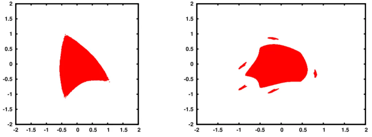
-2 -1.5 -1 -0.5 0 0.5 1 1.5 2 -2 -1.5 -1 -0.5 0 0.5 1 1.5 2 -2 -1.5 -1 -0.5 0 0.5 1 1.5 2 -2 -1.5 -1 -0.5 0 0.5 1 1.5 2
Figure 1. Stable region (dynamical aperture) obtained by direct iteration of the map for ω1= π(
√
5 − 1) (left-panel) and ω1=
√
2 (right-panel).
A similar calculation has been performed also for ω1 = √
2 (the choice of ω1 = √
2 instead of the more usual one ω1 = 2π
√
2 allows to highlight the impact of low-order near-resonances), and is illustrated in synthetic form in section 4.6.
4.1
Numerical evaluation of the dynamical aperture
We start our analysis by computing the evolution of a set of points in a neighbourhood of the origin in order to identify the region where the orbits remained confined for a long but finite time (i.e., the dynamical aperture). To this end we take a square of suitable size filled with 16000 initial points uniformly spaced, and calculate the evolution for 105 iterations. Then we plot the points that remain inside the square. The number 105 is suggested by looking at the results in [7]. The results are reported in figure 1. Our aim is to determine the dynamical aperture using normal form. This will likely be a useful tool in order to investigate the improvement of the dynamical aperture thanks to the control terms.
4.2
Construction of the normal form
The normal form for the map (35) is calculated via algebraic manipulation, representing polynomials with coefficients in complex form. Actually we used a package developed on purpose (see [30]) that we named Xϱ´oνoς. We perform a number r of normalization steps. We note that algebraic manipulation allows us to take values of r which are relatively large. E.g., r = 50 or r = 100 are reachable for a two dimensional map, although for the present purpose we do stop the normalization at r = 20.
Therefore, taking a non-resonant frequency ω, we are lead to consider a map in normal form z′ = TZ ◦ Rωz, where Z = {Z1, . . . , Zr, Qr+1, . . .}. Here Q = {0, . . . , 0, Qr+1, Qr+2, . . .} is a non normalized remainder.
Consider now the functions Ij = (x2j + y2j)/2. They transform as I′ = TZ ◦ RωI =
!
s≥0
EsZRωI , with the operator EZ
hand, in view of Z being in normal form, we have EZ
1 I = . . . = ErZI = 0, because LZ1I = . . . = LZrI = 0. We conclude that for every integer t > 0 we have
(36) |I(t) − I(t − 1)| ≤'' ' ! s>r EsZI(t− 1) ' ' ' .
The sum on the r.h.s. is convergent for every r, with a convergence radius ϱ→ 0 with increasing r.
In an analytic approach we could try to estimate a domain of exponential stability in the spirit of Nekhoroshev’s theorem. However, the analytic estimates, even with the support of algebraic manipulation, turn out to be too pessimistic and actually unpractical. Therefore we look for a heuristic estimate of the stability region in the sense that the orbits are confined in a neighbourhood of the origin for a long time. A similar numerical approach has been previously used in [7] and [8] by computing the fraction of orbits starting in a sphere of a given radius and evolving for a long but finite time without leaving an a priori fixed larger sphere.
4.3
Level curves of the invariant function
We enter now the investigation of the invariant function I(x, y) considering different truncation orders r of the normal form. This will bring into evidence the asymptotic character of the series, i.e., the fact that the radius of the convergence region of the normal form shrinks to zero for increasing r.
We remark that in the normal form coordinates (x′, y′), the invariant function is I = (x′2+ y′2)/2, therefore the invariant curves are just circles. In order to compare the curves with the figures given by the numerical evolution, we apply the transformation z = TX(r)z′, the upper label r denoting the order of normalization. According to the
asymptotic character of the series, we expect that for a given radius ϱ the image of the circle in the original coordinates will be a regular curve, just a deformation of a circle, up to a certain order r(ϱ) depending on ϱ, while at higher order the image will exhibit a more or less strange behavior. Since we have two free parameters, r and ϱ, we draw separate figures for fixed ϱ and for fixed r. In each panel of figure 2 we plot the level curves for a fixed value of ϱ and increasing normalization order r. The four panels correspond to the values ϱ = 0.60, 0.70, 0.75, 0.85 (see caption). The values of ϱ are chosen so as to bring into evidence the asymptotic character of the series. In the upper-left panel, with the lowest value of ϱ, we see that most curves corresponding to orders r = 2, . . . , 18 seem to visually coincide, as expected from a convergent series. However, at r = 20 we see that the curve exhibits a strange behaviour, forming some unexpected loops. The curves would become more and more tangled at higher orders, data not shown. We may say that there is an interval of apparent convergence, in this case up to 18. A similar behaviour shows up for ϱ = 0.70 (upper-right panel) and ϱ = 0.75 (lower-left panel), but the interval of apparent convergence is more and more restricted. E.g., for ϱ = 0.70 the curves corresponding to r = 4, 6, 8, 10 are quite close and still regular, while a loop appears at r = 12. For the higher value ϱ = 0.85 all curves are well separated, so that the phenomenon of apparent convergence completely disappears.
-2 -1.5 -1 -0.5 0 0.5 1 1.5 2 -2 -1.5 -1 -0.5 0 0.5 1 1.5 2 02 04 06 08 10 12 14 16 18 20 -2 -1.5 -1 -0.5 0 0.5 1 1.5 2 -2 -1.5 -1 -0.5 0 0.5 1 1.5 2 02 04 06 08 10 12 14 16 -2 -1.5 -1 -0.5 0 0.5 1 1.5 2 -2 -1.5 -1 -0.5 0 0.5 1 1.5 2 02 04 06 08 10 12 14 -2 -1.5 -1 -0.5 0 0.5 1 1.5 2 -2 -1.5 -1 -0.5 0 0.5 1 1.5 2 02 04 06 08 10 12
Figure 2. Level curves of the invariant function for the uncontrolled map, for different values of ϱ = 0.60, 0.70, 0.75, 0.85. The numbers in the legend correspond to the normalization order r (see text).
-2 -1.5 -1 -0.5 0 0.5 1 1.5 2 -2 -1.5 -1 -0.5 0 0.5 1 1.5 2 0.50 0.55 0.60 0.65 0.70 0.75 0.80 0.85 0.90
Figure 3. Level curves of the invariant function for the uncontrolled map for the normalization order r = 10 and for different values of ϱ as indicated in the legend.
-2 -1.5 -1 -0.5 0 0.5 1 1.5 2 -2 -1.5 -1 -0.5 0 0.5 1 1.5 2 02 04 06 08 10 12 14 16 18 20 -2 -1.5 -1 -0.5 0 0.5 1 1.5 2 -2 -1.5 -1 -0.5 0 0.5 1 1.5 2 02 04 06 08 10 12 14 16 -2 -1.5 -1 -0.5 0 0.5 1 1.5 2 -2 -1.5 -1 -0.5 0 0.5 1 1.5 2 02 04 06 08 10 12 14 -2 -1.5 -1 -0.5 0 0.5 1 1.5 2 -2 -1.5 -1 -0.5 0 0.5 1 1.5 2 02 04 06 08 10
Figure 4. Level curves of the invariant function for the map with the control term F2, for different values of ϱ = 0.60, 0.70, 0.75, 0.85. The numbers in the legend
correspond to the normalization order r (see text).
-2 -1.5 -1 -0.5 0 0.5 1 1.5 2 -2 -1.5 -1 -0.5 0 0.5 1 1.5 2 0.50 0.55 0.60 0.65 0.70 0.75 0.80
Figure 5. Level curves of the invariant function for the controlled map for the normalization order r = 12 and for different values of ϱ as indicated in the legend.
-2 -1.5 -1 -0.5 0 0.5 1 1.5 2 -2 -1.5 -1 -0.5 0 0.5 1 1.5 2 02 04 06 08 10 12 14 16 18 20 -2 -1.5 -1 -0.5 0 0.5 1 1.5 2 -2 -1.5 -1 -0.5 0 0.5 1 1.5 2 02 04 06 08 10 12 14 16 -2 -1.5 -1 -0.5 0 0.5 1 1.5 2 -2 -1.5 -1 -0.5 0 0.5 1 1.5 2 02 04 06 08 10 12 -2 -1.5 -1 -0.5 0 0.5 1 1.5 2 -2 -1.5 -1 -0.5 0 0.5 1 1.5 2 02 04 06 08
Figure 6. Level curves of the invariant function for the map with the control term F3, for different values of ϱ = 0.70, 0.80, 0.90, 1.00. The numbers in the legend
correspond to the normalization order r (see text).
-2 -1.5 -1 -0.5 0 0.5 1 1.5 2 -2 -1.5 -1 -0.5 0 0.5 1 1.5 2 0.60 0.65 0.70 0.75 0.80 0.85 0.90 0.95 1.00 1.05
Figure 7. Level curves of the invariant function for the controlled map for the normalization order r = 8 and for different values of ϱ as indicated in the legend.
-2 -1.5 -1 -0.5 0 0.5 1 1.5 2 -2 -1.5 -1 -0.5 0 0.5 1 1.5 2 02 04 06 08 10 12 14 16 18 20 -2 -1.5 -1 -0.5 0 0.5 1 1.5 2 -2 -1.5 -1 -0.5 0 0.5 1 1.5 2 02 04 06 08 10 12 14 16 18 -2 -1.5 -1 -0.5 0 0.5 1 1.5 2 -2 -1.5 -1 -0.5 0 0.5 1 1.5 2 02 04 06 08 10 12 14 16 -2 -1.5 -1 -0.5 0 0.5 1 1.5 2 -2 -1.5 -1 -0.5 0 0.5 1 1.5 2 02 04 06 08 10
Figure 8. Level curves of the invariant function for the the map with the control term F4, for different values of ϱ = 0.70, 0.75, 0.80, 0.90. The numbers in the
legend correspond to the normalization order r (see text).
-2 -1.5 -1 -0.5 0 0.5 1 1.5 2 -2 -1.5 -1 -0.5 0 0.5 1 1.5 2 0.50 0.55 0.60 0.65 0.70 0.75 0.80 0.85 0.90
Figure 9. Level curves of the invariant function for the controlled map for the normalization order r = 12 and for different values of ϱ as indicated in the legend.
-2 -1.5 -1 -0.5 0 0.5 1 1.5 2 -2 -1.5 -1 -0.5 0 0.5 1 1.5 2 10 0.75 10 0.80 -2 -1.5 -1 -0.5 0 0.5 1 1.5 2 -2 -1.5 -1 -0.5 0 0.5 1 1.5 2 12 0.70 12 0.75 -2 -1.5 -1 -0.5 0 0.5 1 1.5 2 -2 -1.5 -1 -0.5 0 0.5 1 1.5 2 08 0.90 08 0.95 -2 -1.5 -1 -0.5 0 0.5 1 1.5 2 -2 -1.5 -1 -0.5 0 0.5 1 1.5 2 12 0.70 12 0.75
Figure 10. Comparison of the level curves of the invariant functions with the stability zone obtained by direct iteration of the map (with ω1= π(
√
5 − 1)). The four panels (left to right) correspond to the uncontrolled map and the three different controls F2, F3 and F4. The normalization order r and the radius ϱ are selected
using the heuristic criterion illustrated in subsection 4.3. We plot the level curves for two different values of ϱ. The lower one produces a reliable approximation of the stability zone. One sees that the best control terms is F3 (left-lower panel).
choice r = 10 is suggested by the preliminary analysis performed on figure 2 (see lower-left panel of such figure). As we see, for ϱ = 0.9 the curve exibits a loop, thus showing that we are out of the radius of apparent convergence. Thus we may consider the interval Iϱ = (0.7−0.8) as the right one, and we may make a safe choice with ϱ = 0.75.
The comparison between the two figures provides us with a heuristic criterion in order to make a safe choice of ϱ, which is the relevant quantity for the dynamics. A corresponding value of r is also suggested. The aim of the next section is to compare the improved behaviour and the optimality of the controlled map against the uncontrolled one using such heuristic metrics: ϱ and r.
4.4
Level curves for the controlled map
We illustrate the application of the criterion above by introducing different corrections to the map.
-2 -1.5 -1 -0.5 0 0.5 1 1.5 2 -2 -1.5 -1 -0.5 0 0.5 1 1.5 2 08 0.70 08 0.75 -2 -1.5 -1 -0.5 0 0.5 1 1.5 2 -2 -1.5 -1 -0.5 0 0.5 1 1.5 2 06 1.00 06 1.05 -2 -1.5 -1 -0.5 0 0.5 1 1.5 2 -2 -1.5 -1 -0.5 0 0.5 1 1.5 2 06 1.00 06 1.05 -2 -1.5 -1 -0.5 0 0.5 1 1.5 2 -2 -1.5 -1 -0.5 0 0.5 1 1.5 2 06 1.05 06 1.10
Figure 11. Comparison of the level curves of the invariant functions with the stability zone obtained by direct iteration of the map (with ω1 =
√
2). See caption of figure 10.
different cases by choosing the control terms F2 ={0, F2, 0, . . .}, F3 ={0, F2, F3, 0, . . .} and F4 ={0, F2, F3, F4, 0, . . .}, with Fs given by (20). This corresponds to introducing controls including increasing orders.
The results for the map with the control term F2 are illustrated in figures 4 for fixed values of ϱ (analogous to figure 2 for the uncontrolled map) and 5 for a fixed value of r = 12 (analogous to figure 3). Looking at the latter figure, we may consider as acceptable a value ϱ in the interval 0.65–0.75.
Similar figures are reported also for the control term F3 in 5–7 and F4 in 8–9. In the former case our heuristic criterion suggests the value ϱ ≃ 0.9, in the latter case we get ϱ ≃ 0.7. Thus it seems reasonable to conclude that the optimal control term, to achieve a good compromise between to have a large ϱ but relatively not so large r, is F3.
4.5
Comparison with the dynamics
We now compare the level curves of the invariant function with the results of the dy-namics obtained by direct numerical iteration of the map (see subsection 4.1).
For the uncontrolled map and the three controlled map considered above, we su-perimpose to the effectively stable points defined above, the level curves corresponding
to ϱ = 0.75 for the uncontrolled map, ϱ = 0.70 for the control term F2, ϱ = 0.90 for the control term F3 and ϱ = 0.70 for the control term F4. The results are reported in figure 10. As one sees there is a good agreement between the dynamical aperture suggested by the dynamics and the one estimated via the normal form. For comparison we also add the level curves for values of ϱ slightly bigger than the good estimated ones, thus showing that actually our heuristic criterion produces reliable hints.
4.6 Changing the rotation number
As anticipated, we performed a complete calculation for the case ω1 = √
2. The resulting figures for the level curves at different values of ϱ and r exhibit a behaviour similar to figures 2–10. Thus we do not include a complete set of figures, reporting only the final results in figure 11 (corresponding to figure 10 of the previous section).
Acknowledgements.
A. G. and M. S. have been partially supported by the research program “Teorie geometriche e analitiche dei sistemi Hamiltoniani in dimen-sioni finite e infinite”, PRIN 2010JJ4KPA 009, financed by MIUR. The work of T.C. presents research results of the Belgian Network DYSCO (Dynamical Systems, Control, and Optimization), funded by the Interuniversity Attraction Poles Programme, initiated by the Belgian State, Science Policy Office.References
[1] A. Bazzani, P. Mazzanti, G. Servizi, G. Turchetti: Normal forms for Hamiltonian maps and nonlinear effects in a particle accelerator, Nuovo Cim. B, 102, 51–80 (1988).
[2] A. Bazzani, M. Giovannozzi, G. Servizi, E. Todesco, G. Turchetti: Resonant normal forms, interpolating Hamiltonians and stability of area preserving maps, Physica D, 64, 66–93 (1993).
[3] A. Bazzani, E. Todesco, G. Turchetti: A normal form approach to the theory of nonlinear betatronic motion, CERN Report No.94-02 (1994).
[4] G. Benettin, L. Galgani, A. Giorgilli: A proof of Nekhoroshev’s theorem for the stability times in nearly integrable Hamiltonian systems. Cel. Mech., 37, 1–25 (1985).
[5] G.D. Birkhoff: Surface transformations and thair dynamical applications, Acta Mathematica, 43, 1–119 (1920).
[6] G.D. Birkhoff: Dynamical systems, New York (1927).
[7] J. Boreux, T. Carletti, C. Skokos, Y. Papaphilippou, M. Vittot: Efficient control of accelerator maps, International Journal of Bifurcation and Chaos, 22 (9), 1250219-1–1250219-9 (2012).
[8] J. Boreux, T. Carletti, C. Skokos, M. Vittot: Hamiltonian control used to improve the beam stability in particle accelerator models, Communications in Nonlinear Science and Numerical Simulation, 17, 1725–1738 (2012).
[9] T. Bountis and C. Skokos: Space charges can significantly affect the dynamics of accelerator maps, Phys. Lett. A, 358, 126133 (2006).
[10] F. Callier and C. Desoer: Linear system theory, Springer-Verlag, (1991).
[11] A. Celletti and L. Chierchia: Construction of analytic KAM surfaces and effective stability bounds, Communications in Mathematical Physics, 118, 119–161 (1988). [12] A. Celletti, L. Chierchia: On the stability of realistic three-body problems,
Com-munications in Mathematical Physics, 186, 413–449 (1997).
[13] T.M. Cherry: On integrals developable about a singular point of a Hamiltonian system of differential equations, Proc. Camb. Phil. Soc., 22, 325–349 (1924). [14] T.M. Cherry: On integrals developable about a singular point of a Hamiltonian
system of differential equations, II, Proc. Camb. Phil. Soc., 22 510–533 (1924). [15] G. Ciraolo, F. Briolle, C. Chandre, E. Floriani, R. Lima, M. Vittot, M. Pettini:
Control of Hamiltonian chaos as a possible tool to control anomalous transport in fusion plasmas Physical Review E, 69 (5), 056213 (2004).
[16] G. Ciraolo, C. Chandre, R. Lima, M. Vittot, M. Pettini: Control of chaos in Hamiltonian systems CeMDA, 90, 3-12 (2004).
[17] G. Ciraolo, C. Chandre, R. Lima, M. Vittot, M. Pettini, C. Figarella, P. Ghen-drih: Controlling chaotic transport in a Hamiltonian model of interest to magne-tized plasmas, Journal of Physics A 37, 3589 (2004).
[18] A. Deprit: Canonical transformations depending on a small parameter, Cel. Mech., 1, 12–30 (1969).
[19] F. Fass`o: On a relation among Lie series , Cel. Mech., 46, 113–118 (1989). [20] G. Gallavotti: A criterion of of integrability for perturbed nonresonant harmonic
oscillators. “Wick ordering” of the perturbations in Calssical Mechanics and in-variance in the frequency spectrum, Comm. Math. Phys., 87, 365–383 (1982). [21] A. Giorgilli and L. Galgani: Formal integrals for an autonomous Hamiltonian
system near an equilibrium point, Cel. Mech., 17, 267–280 (1978).
[22] A. Giorgilli and L. Galgani: Rigorous estimates for the series expansions of Hamiltonian perturbation theory, Cel. Mech., 37, 95–112 (1985).
[23] A. Giorgilli and E. Zehnder: Exponential stability for time dependent potentials, ZAMP, 5, 827–855 (1992).
[24] A. Morbidelli and A. Giorgilli: Superexponential stability of KAM tori, J. Stat. Phys., 78, 1607–1617 (1995).
[25] A. Morbidelli and A. Giorgilli: On a connection between KAM and Nekhoroshev’s theorem, Physica D, 86, 514–516 (1995).
[26] A. Giorgilli and Ch. Skokos: On the stability of the Trojan asteroids, Astron. Astroph., 317, 254–261 (1997).
[27] A. Giorgilli: Notes on exponential stability of Hamiltonian systems, in Dynamical Systems, Part I. Pubbl. Cent. Ric. Mat. Ennio De Giorgi, Sc. Norm. Sup. Pisa, 87–198 (2003).
[28] A. Giorgilli, U. Locatelli, M. Sansottera: Kolmogorov and Nekhoroshev theory for the problem of three bodies, CeMDA, 104, 159–175 (2009).
dell’Istituto Lombardo Accademia di Scienze e Lettere, Classe di Scienze Matem-atiche e Naturali, to appear (see also arXiv:1211.5674).
[30] A. Giorgilli and M. Sansottera: Methods of algebraic manipulation in perturbation theory, Workshop Series of the Asociacion Argentina de Astronomia, 3, 147–183 (2011).
[31] W. Gr¨obner: Nuovi contributi alla teoria dei sistemi di equazioni differenziali nel campo analitico, Atti Accad. Naz. Lincei. Rend. Cl. Sci. Fis. Mat. Nat., 23, 375-379 (1957).
[32] W. Gr¨obner: Die Lie-Reihen und Ihre Anwendungen, VEB Deutscher Verlag der Wissenschaften, Berlin (1967).
[33] J. Hanson and J. Cary: Elimination of stochasticity in stellerators, Physics of fluids, 27, 767–769, (1984).
[34] J. Henrard and J. Roels: Equivalence for Lie transforms, Cel. Mech., 10, 497–512 (1974).
[35] D. Hinrichsen and A. Pritchard: Mathematical systems theory I modelling, state space analysis, stability and robustness, Springer-Verlag, (2005).
[36] G. Hori: Theory of general perturbations with unspecified canonical variables, Publ. Astron. Soc. Japan, 18, 287–296 (1966).
[37] J.E. Littlewood: On the equilateral configuration in the restricted problem of three bodies, Proc. London Math. Soc.(3), 9, 343–372 (1959).
[38] J.E. Littlewood: The Lagrange configuration in celestial mechanics, Proc. London Math. Soc.(3), 9, 525–543 (1959).
[39] A. Locatelli: Optimal control: an introduction., Birkha¨user (2001)
[40] A.N. Kolmogorov: Preservation of conditionally periodic movements with small change in the Hamilton function, Dokl. Akad. Nauk SSSR, 98, 527 (1954). En-glish translation in: Los Alamos Scientific Laboratory translation LA-TR-71-67; reprinted in: G. Casati, J. Ford: Stochastic behavior in classical and quantum Hamiltonian systems, Lecture Notes in Physics, 93, 51–56 (1979).
[41] U. Locatelli and A. Giorgilli: Invariant tori in the secular motions of the three-body planetary systems, Cel. Mech., 78, 47–74 (2000).
[42] U. Locatelli and A. Giorgilli: Invariant tori in the Sun-Jupiter-Saturn system, DCDS-B, 7, 377–398 (2007).
[43] J. Moser: Stabilit¨atsverhalten kanonisher differentialgleichungssysteme, Nachr. Akad. Wiss. G¨ottingen, Math. Phys. K1. IIa, 6 87–120 (1955).
[44] N.N. Nekhoroshev: Exponential estimates of the stability time of near-integrable Hamiltonian systems. English translation: Russ. Math. Surveys, 32, 1 (1977). [45] N.N. Nekhoroshev: Exponential estimates of the stability time of near-integrable
Hamiltonian systems, 2. Trudy Sem. Im. G. Petrovskogo, 5, 5 (1979). English translation: Topics in modern Mathematics, Petrovskij Semin., 5, 1–58 (1985). [46] H. Poincar´e: Sur le probl`eme des trois corps et les ´equations de la dynamique,
Acta Mathematica (1890).
[47] H. Poincar´e: Les m´ethodes nouvelles de la m´ecanique c´eleste, Gauthier-Villars, Paris (1892).