Multifactorial Exploratory Approaches: multiple correspondence analysis

(1)

HAL Id: halshs-02908477

https://halshs.archives-ouvertes.fr/halshs-02908477

Submitted on 29 Jul 2020

HAL is a multi-disciplinary open access

archive for the deposit and dissemination of

sci-entific research documents, whether they are

pub-lished or not. The documents may come from

teaching and research institutions in France or

abroad, or from public or private research centers.

L’archive ouverte pluridisciplinaire HAL, est

destinée au dépôt et à la diffusion de documents

scientifiques de niveau recherche, publiés ou non,

émanant des établissements d’enseignement et de

recherche français ou étrangers, des laboratoires

publics ou privés.

Multifactorial Exploratory Approaches: multiple

correspondence analysis

Guillaume Desagulier

To cite this version:

Guillaume Desagulier. Multifactorial Exploratory Approaches: multiple correspondence analysis.

École thématique. United Kingdom. 2019. �halshs-02908477�

(2)

outline introduction principles case study References

Multifactorial Exploratory Approaches

multiple correspondence analysis

Guillaume Desagulier1

1_{MoDyCo (UMR 7114)}

Paris 8, CNRS, Paris Nanterre Institut Universitaire de France gdesagulier@univ-paris8.fr

Corpus Linguistics Summer School 2019 June 25th_{, 2019}

University of Birmingham

(3)

outline

1 introduction

2 principles

(4)

MCA

Because MCA is an extension of CA, its inner workings are very similar. For this reason, they are not repeated here.

(5)

nominal data

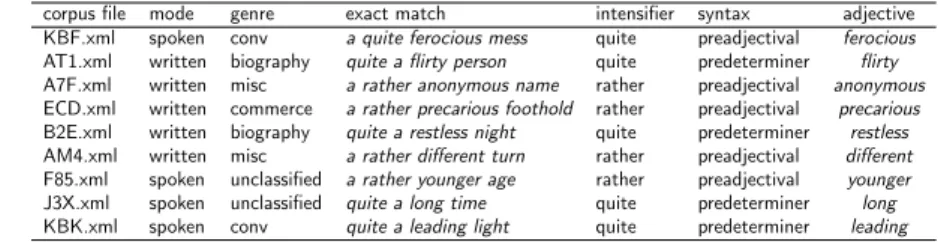
As pointed out yesterday, MCA takes as input a table ofnominal data.

Table 1:A sample input table for MCA (Desagulier 2017, p. 36)

corpus file mode genre exact match intensifier syntax adjective KBF.xml spoken conv a quite ferocious mess quite preadjectival ferocious AT1.xml written biography quite a flirty person quite predeterminer flirty A7F.xml written misc a rather anonymous name rather preadjectival anonymous ECD.xml written commerce a rather precarious foothold rather preadjectival precarious B2E.xml written biography quite a restless night quite predeterminer restless AM4.xml written misc a rather different turn rather preadjectival different F85.xml spoken unclassified a rather younger age rather preadjectival younger J3X.xml spoken unclassified quite a long time quite predeterminer long KBK.xml spoken conv quite a leading light quite predeterminer leading

(6)

beware of inertia

For MCA to yield manageable results, it is best if

• the table is of reasonable size (not too many columns) • each variable does not break down into too many categories

Otherwise, the contribution of each dimension to φ2_{is small, and a large}

number of dimensions must be inspected(which kind of defeats the purpose)

(7)

beware of inertia

There are no hard and fast rules for knowing when there are too many dimensions to inspect.

However, when the eigenvalue that corresponds to a dimension is low, we know that the dimension is of little interest (the chances are that the data points will be close to the intersection of the axes in the summary plot).

(8)

how men and women swear in the BNC-XML

Schmid (2003) provides an analysis of sex differences in the 10M-word spoken section of the British National Corpus (BNC). Schmid shows that women use certain swear-words more than men, although swear-words which tend to have a perceived ‘strong’ effect are more frequent in male speech. Schmid’s study is based on two subcorpora, which are both sampled from the spoken section of the BNC. The subcorpora amount to 8,173,608 words.

(9)

how men and women swear in the BNC-XML

The contributions are not equally shared among men and women since for every 100 word spoken by women, 151 are spoken by men. To calculate the distinctive lexical preferences of men and women, while taking the lack of balance in the contributions into account, Schmid’s measures rely on the difference coefficient.

(10)

how men and women swear in the BNC-XML

This formula is based on normalized frequencies per million words. Its score ranges from -1 (if a word occurs more frequently in women’s utterances) to 1 (if a word occurs more frequently in male speech). Absolute frequencies are used to calculate the significance level of the differences using the hypergeometrical approximation of the binomial distribution. With respect to swear-words, Schmid’s conclusion is that

both men and women swear, but men tend to use stronger swear-words than women.

(11)

how men and women swear in the BNC-XML

Schmid’s study is repeated here in order to explore the distribution of swear-words with respect to gender in the BNC-XML. The goal is to see if:

• men swear more than women;

• some swear-words are preferred by men or women;

• the gender-distribution of swear-words is correlated with other variables: age and social class.

(12)

how men and women swear in the BNC-XML

The code for the extraction was partly contributed by Mathilde Léger, a third-year student at Paris 8 University, as part of her end-of-term project. Unlike Schmid, and following Rayson et al. (1997), the data are extracted from the demographic component of the BNC-XML, which consists of spontaneous interactive discourse. The swear-words are: bloody, damn, fuck, fucked, fucker, fucking, gosh, and shit.

Two exploratory variables are included: age and social class.

(13)

how men and women swear in the BNC-XML

> # clear R's memory > rm(list=ls(all=TRUE)) > #load FactoMineR > library(FactoMineR)

> # load the data (choose swearwords_bnc.txt)

(14)

how men and women swear in the BNC-XML

The data set contains 293,289 swear-words. These words are described by three categorical variables (nominal data):

• gender (2 levels: male and female)

• age (6 levels: Ag0, Ag1, Ag2, Ag3, Ag4, Ag5) • social class (4 levels: AB, C1, C2, DE)

(15)

how men and women swear in the BNC-XML

Agebreaks down into 6 groups:

• Ag0: respondent age between 0 and 14; • Ag1: respondent age between 15 and 24; • Ag2: respondent age between 25 and 34; • Ag3: respondent age between 35 and 44; • Ag4: respondent age between 45 and 59; • Ag5: respondent age is 60+.

Social classesare divided into 4 groups:

• AB: higher management: administrative or professional. • C1: lower management: supervisory or clerical;

(16)

how men and women swear in the BNC-XML

It is advisable to keep an eye on the number of levels for each variable and see if any can be kept to a minimum to guarantee that inertia will not drop.

> str(df)

'data.frame': 293289 obs. of 4 variables:

$ word : Factor w/ 8 levels "bloody","damn",..: 2 2 7 7 7 2 7 2 7 7 ... $ gender : Factor w/ 2 levels "f","m": 2 2 2 2 2 2 2 2 2 2 ...

$ age : Factor w/ 6 levels "Ag0","Ag1","Ag2",..: 6 6 6 6 6 6 6 6 6 6 ... $ soc_class: Factor w/ 4 levels "AB","C1","C2",..: 1 1 1 1 1 1 1 1 1 1 ... > table(df$word)

bloody damn fuck fucked fucker fucking gosh shit 146203 32294 9219 11 467 23487 60678 20930

(17)

how men and women swear in the BNC-XML

We can group fuck, fucking, fucked, and fucker into a single factor: f-words. With gsub(), we replace each word with the single tag f-words.

> df$word <- gsub("fuck|fucking|fucker|fucked", "f-words", df$word, ignore.case=TRUE) > table(df$word)

bloody damn f-words gosh shit 146203 32294 33184 60678 20930

We convert df$word back to a factor. The number of levels has been reduced to five.

(18)

How men and women swear in the BNC-XML

As in CA, we can declare some variables as active and some other variables as supplementary/illustrative in MCA. We declare the variables corresponding to swear words and gender as active, and the variables age and social class as supplementary/illustrative.

Running a MCA involves the following steps:

• determining how many dimensions there are to inspect; • interpreting the MCA graph.

(19)

How men and women swear in the BNC-XML

We run the MCA with the MCA() function. We declare age and

soc_class as supplementary (quali.sup=c(3,4)). We do not plot the graph yet (graph=FALSE).

> mca.object <- MCA(df, quali.sup=c(3,4), graph=FALSE)

Again, the eig object allows us to see how many dimensions there are to inspect.

> round(mca.object$eig, 2)

eigenvalue percentage of variance cumulative percentage of variance

dim 1 0.56 22.47 22.47

dim 2 0.50 20.00 42.47

dim 3 0.50 20.00 62.47

(20)

How men and women swear in the BNC-XML

The number of dimensions is rather large and the first two dimensions account for only 42.47% of φ2_{. To inspect a significant share of φ}2_{, e.g.}

80%, we would have to inspect at least 4 dimensions. This issue is common in MCA. The eigenvalues can be vizualized by means of a scree plot. It is obtained as follows.

> barplot(mca.object$eig[,1],

+ names.arg=paste("dim ", 1:nrow(mca.object$eig)), las=2)

(21)

How men and women swear in the BNC-XML

dim 1 dim 2 dim 3 dim 4 dim 5

0.0 0.1 0.2 0.3 0.4 0.5

(22)

How men and women swear in the BNC-XML

The MCA map is plotted with the plot.MCA() function. Each category is the color of its variable (habillage="quali"). The title is removed (title=""). > plot.MCA(mca.object, + invisible="ind", + autoLab="yes", + shadowtext=TRUE, + habillage="quali", + title="")

(23)

How men and women swear in the BNC-XML

−1

0

1

2

MCA factor map

Dim 2 (20.00%) bloody f−words gosh shit f m Ag0 Ag1 Ag2 Ag3 Ag4 Ag5 AB C1 C2 DE bloody f−words gosh shit f m Ag0 Ag1 Ag2 Ag3 Ag4 Ag5 AB C1 C2 DE bloody f−words gosh shit f m Ag0 Ag1 Ag2 Ag3 Ag4 Ag5 AB C1 C2 DE bloody f−words gosh shit f m Ag0 Ag1 Ag2 Ag3 Ag4 Ag5 AB C1 C2 DE bloody f−words gosh shit f m Ag0 Ag1 Ag2 Ag3 Ag4 Ag5 AB C1 C2 DE bloody f−words gosh shit f m Ag0 Ag1 Ag2 Ag3 Ag4 Ag5 AB C1 C2 DE bloody f−words gosh shit f m Ag0 Ag1 Ag2 Ag3 Ag4 Ag5 AB C1 C2 DE bloody f−words gosh shit f m Ag0 Ag1 Ag2 Ag3 Ag4 Ag5 AB C1 C2 DE bloody f−words gosh shit f m Ag0 Ag1 Ag2 Ag3 Ag4 Ag5 AB C1 C2 DE

(24)

How men and women swear in the BNC-XML

dim 1 −1 0 1 2 −2 −1 0 1 2

MCA factor map

Dim 1 (22.47%) Dim 2 (20.00%) bloody damn f−words gosh shit f m Ag0 Ag1 Ag2 Ag3 Ag4 Ag5 AB C1 C2 DE bloody damn f−words gosh shit f m Ag0 Ag1 Ag2 Ag3 Ag4 Ag5 AB C1 C2 DE bloody damn f−words gosh shit f m Ag0 Ag1 Ag2 Ag3 Ag4 Ag5 AB C1 C2 DE bloody damn f−words gosh shit f m Ag0 Ag1 Ag2 Ag3 Ag4 Ag5 AB C1 C2 DE bloody damn f−words gosh shit f m Ag0 Ag1 Ag2 Ag3 Ag4 Ag5 AB C1 C2 DE bloody damn f−words gosh shit f m Ag0 Ag1 Ag2 Ag3 Ag4 Ag5 AB C1 C2 DE bloody damn f−words gosh shit f m Ag0 Ag1 Ag2 Ag3 Ag4 Ag5 AB C1 C2 DE bloody damn f−words gosh shit f m Ag0 Ag1 Ag2 Ag3 Ag4 Ag5 AB C1 C2 DE bloody damn f−words gosh shit f m Ag0 Ag1 Ag2 Ag3 Ag4 Ag5 AB C1 C2 DE

Strikingly, the most explicit swear words (f-words) cluster in the right-most part of the plot. These are used mostly by men. Female speakers tend to prefer a softer swear word: bloody.

(25)

How men and women swear in the BNC-XML

dim 2 −2 −1 0 1 2

MCA factor map

Dim 2 (20.00%) bloody damn f−words gosh shit f m Ag0 Ag1 Ag2 Ag3 Ag4 Ag5 AB C1 C2 DE bloody damn f−words gosh shit f m Ag0 Ag1 Ag2 Ag3 Ag4 Ag5 AB C1 C2 DE bloody damn f−words gosh shit f m Ag0 Ag1 Ag2 Ag3 Ag4 Ag5 AB C1 C2 DE bloody damn f−words gosh shit f m Ag0 Ag1 Ag2 Ag3 Ag4 Ag5 AB C1 C2 DE bloody damn f−words gosh shit f m Ag0 Ag1 Ag2 Ag3 Ag4 Ag5 AB C1 C2 DE bloody damn f−words gosh shit f m Ag0 Ag1 Ag2 Ag3 Ag4 Ag5 AB C1 C2 DE bloody damn f−words gosh shit f m Ag0 Ag1 Ag2 Ag3 Ag4 Ag5 AB C1 C2 DE bloody damn f−words gosh shit f m Ag0 Ag1 Ag2 Ag3 Ag4 Ag5 AB C1 C2 DE bloody damn f−words gosh shit f m Ag0 Ag1 Ag2 Ag3 Ag4 Ag5 AB C1 C2 DE

Words in the upper part (gosh and shit) are used primarily by upper-class speakers. F-words, bloody, and damn are used by lower social categories. Age groups are positioned close to the intersection of the axes. This is a sign that the first two dimensions bring little or no information about them.

(26)

How men and women swear in the BNC-XML

dim 1 + dim 2 −1 0 1 2 −2 −1 0 1 2

MCA factor map

Dim 1 (22.47%) Dim 2 (20.00%) bloody damn f−words gosh shit f m Ag0 Ag1 Ag2 Ag3 Ag4 Ag5 AB C1 C2 DE bloody damn f−words gosh shit f m Ag0 Ag1 Ag2 Ag3 Ag4 Ag5 AB C1 C2 DE bloody damn f−words gosh shit f m Ag0 Ag1 Ag2 Ag3 Ag4 Ag5 AB C1 C2 DE bloody damn f−words gosh shit f m Ag0 Ag1 Ag2 Ag3 Ag4 Ag5 AB C1 C2 DE bloody damn f−words gosh shit f m Ag0 Ag1 Ag2 Ag3 Ag4 Ag5 AB C1 C2 DE bloody damn f−words gosh shit f m Ag0 Ag1 Ag2 Ag3 Ag4 Ag5 AB C1 C2 DE bloody damn f−words gosh shit f m Ag0 Ag1 Ag2 Ag3 Ag4 Ag5 AB C1 C2 DE bloody damn f−words gosh shit f m Ag0 Ag1 Ag2 Ag3 Ag4 Ag5 AB C1 C2 DE bloody damn f−words gosh shit f m Ag0 Ag1 Ag2 Ag3 Ag4 Ag5 AB C1 C2 DE

we observe 3 distinct clusters:

cluster 1(upper-right corner) gosh and shit, used by male and female upper class speakers;

cluster 2(lower-left corner) bloody, used by female middle-class speakers;

cluster 3(lower-right corner) f-words and damn, used by male lower-class speakers.

(27)

How men and women swear in the BNC-XML

A divide exists between male (m, right) and female (f, left) speakers. However, as the combined eigenvalues indicate, we should be wary of making final conclusions based on the sole inspection of the first two dimensions. The relevance of age groups becomes more relevant if dimensions 3 and 4 are inspected together

> plot.MCA(mca.object, + axes=c(3,4), + invisible="ind", + autoLab="yes", + shadowtext=TRUE, + habillage="quali", + title="")

(28)

How men and women swear in the BNC-XML

−2 −1 0 1 2 3 0 1 2 3 4

MCA factor map

Dim 3 (20.00%) Dim 4 (20.00%) bloody damn f−words gosh shit fm Ag0 Ag1 Ag2 Ag3 Ag4 Ag5 AB C1 C2 DE bloody damn f−words gosh shit fm Ag0 Ag1 Ag2 Ag3 Ag4 Ag5 AB C1 C2 DE bloody damn f−words gosh shit fm Ag0 Ag1 Ag2 Ag3 Ag4 Ag5 AB C1 C2 DE bloody damn f−words gosh shit fm Ag0 Ag1 Ag2 Ag3 Ag4 Ag5 AB C1 C2 DE bloody damn f−words gosh shit fm Ag0 Ag1 Ag2 Ag3 Ag4 Ag5 AB C1 C2 DE bloody damn f−words gosh shit fm Ag0 Ag1 Ag2 Ag3 Ag4 Ag5 AB C1 C2 DE bloody damn f−words gosh shit fm Ag0 Ag1 Ag2 Ag3 Ag4 Ag5 AB C1 C2 DE bloody damn f−words gosh shit fm Ag0 Ag1 Ag2 Ag3 Ag4 Ag5 AB C1 C2 DE bloody damn f−words gosh shit fm Ag0 Ag1 Ag2 Ag3 Ag4 Ag5 AB C1 C2 DE

(29)

How men and women swear in the BNC-XML

dim 3 + dim 4 0 1 2 3 4

MCA factor map

Dim 4 (20.00%) bloody damn f−words gosh shit fm Ag0 Ag1 Ag2 Ag3 Ag4 Ag5 AB C1 C2 DE bloody damn f−words gosh shit fm Ag0 Ag1 Ag2 Ag3 Ag4 Ag5 AB C1 C2 DE bloody damn f−words gosh shit fm Ag0 Ag1 Ag2 Ag3 Ag4 Ag5 AB C1 C2 DE bloody damn f−words gosh shit fm Ag0 Ag1 Ag2 Ag3 Ag4 Ag5 AB C1 C2 DE bloody damn f−words gosh shit fm Ag0 Ag1 Ag2 Ag3 Ag4 Ag5 AB C1 C2 DE bloody damn f−words gosh shit fm Ag0 Ag1 Ag2 Ag3 Ag4 Ag5 AB C1 C2 DE bloody damn f−words gosh shit fm Ag0 Ag1 Ag2 Ag3 Ag4 Ag5 AB C1 C2 DE bloody damn f−words gosh shit fm Ag0 Ag1 Ag2 Ag3 Ag4 Ag5 AB C1 C2 DE bloody damn f−words gosh shit fm Ag0 Ag1 Ag2 Ag3 Ag4 Ag5 AB C1 C2 DE

• the male/female distinction disappears

• a divide is observed between f-words and bloody (left), used mostly by younger and

middle-aged speakers, and gosh and damn (right), used mostly by upper-class speakers from age groups 3 and 5.

• the most striking feature is the outstanding position of shit in

(30)

Practical Handbook of Corpus Linguistics

Guillaume Desagulier (to appear). “Multifactorial exploratory approaches.” In: Practical Handbook of Corpus Linguistics. Ed. by Magali Paquot and Stefan Thomas Gries. New York: Springer

(31)

Corpus Linguistics and Statistics with R

springer.com

1st ed. 2017, XIII, 353 p. 98 illus., 55 illus. in color. Printed book Hardcover 79,99 € | £69.99 | $99.99 85,59 € (D) | 87,99 € (A) | CHF [1] 88,00 eBook 67,82 € | £55.99 | $79.99 67,82 € (D) | 67,82 € (A) | CHF [2] 70,00

Available from your library or springer.com/shop

MyCopy [3]

Printed eBook for just € | $ 24.99 springer.com/mycopy

Guillaume Desagulier

Corpus Linguistics and

Statistics with R

Introduction to Quantitative Methods in Linguistics

Series: Quantitative Methods in the Humanities and Social Sciences Accessible introduction to quantitative methods for linguistics with emphasis on learning the methods and then applying them with R

Includes downloadable supplementary materials for readers

Suitable for advanced undergraduate courses, graduate courses, and self-study

This textbook examines empirical linguistics from a theoretical linguist’s perspective. It provides both a theoretical discussion of what quantitative corpus linguistics entails and detailed, hands-on, step-by-step instructions to implement the techniques in the field. The statistical methodology and R-based coding from this book teach readers the basic and then more advanced skills to work with large data sets in their linguistics research and studies. Massive data sets are now more than ever the basis for work that ranges from usage-based linguistics to the far reaches of applied linguistics. This book presents much of the methodology in a corpus-based approach. However, the corpus-based methods in this book are also essential components of recent developments in sociolinguistics, historical linguistics, computational linguistics, and psycholinguistics. Material from the book will also be appealing to researchers in digital humanities and the many non-linguistic fields that use textual data analysis and text-based sensorimetrics. Chapters cover topics including corpus processing, frequencing data, and clustering methods. Case studies illustrate each chapter with accompanying data sets, R code, and exercises for use by readers. This book may be used in advanced undergraduate courses, graduate courses, and self-study.

Section 10.5 – (Desagulier 2017)

(32)

Bibliography I

Desagulier, Guillaume (to appear).“Multifactorial exploratory approaches.” In: Practical Handbook of Corpus Linguistics. Ed. by Magali Paquot and Stefan Thomas Gries. New York: Springer.

– (2017).“Clustering Methods.” In: Corpus Linguistics and Statistics with R. New York, NY: Springer, pp. 239–294.

Rayson, Paul, Geoffrey N Leech, and Mary Hodges (1997).“Social differentiation in the use of English vocabulary: some analyses of the conversational component of the British National Corpus.” In: International Journal of Corpus Linguistics 2.1, pp. 133–152.

Schmid, Hans Jörg (2003).“Do men and women really live in different cultures? Evidence from the BNC.” In: Corpus Linguistics by the Lune. Ed. by Andrew Wilson, Paul Rayson, and Tony McEnery. Lódź Studies in Language. Frankfurt: Peter Lang, pp. 185–221.