A Comprehensive Assessment of Markets for Frequency and Voltage Control Ancillary Services

HAL Id: tel-00370805

https://tel.archives-ouvertes.fr/tel-00370805

Submitted on 25 Mar 2009

HAL is a multi-disciplinary open access

archive for the deposit and dissemination of sci-entific research documents, whether they are pub-lished or not. The documents may come from teaching and research institutions in France or abroad, or from public or private research centers.

L’archive ouverte pluridisciplinaire HAL, est destinée au dépôt et à la diffusion de documents scientifiques de niveau recherche, publiés ou non, émanant des établissements d’enseignement et de recherche français ou étrangers, des laboratoires publics ou privés.

Yann Rebours

To cite this version:

Yann Rebours. A Comprehensive Assessment of Markets for Frequency and Voltage Control Ancillary Services. Electric power. University of Manchester, 2008. English. �tel-00370805�

A Comprehensive Assessment of

Markets for Frequency and

Voltage Control Ancillary

Services

A thesis submitted to The University of Manchester for the degree of

Doctor of Philosophy

in the Faculty of Engineering and Physical Sciences

2008

Yann Rebours

3

CONTENTS

Contents 3

List of tables

9

List of figures

11

Abstract 17

Declaration 19

Copyright 21

Acknowledgement 23

Abbreviations and acronyms

25

Symbols 33

Chapter 1 Introduction

43

1.1

Increasing Welfare of Power System Users

43

1.2

Stakeholders 46

1.3

Marketplaces 49

1.3.1 Basic features of a marketplace 49

1.3.3 Transmission markets 53

1.3.4 Retail markets 54

1.3.5 Other markets 54

1.4

Fundamentals of Frequency Control

55

1.4.1 Frequency and active power 55 1.4.2 Dynamic and quasi-steady-state frequency deviations 57 1.4.3 Self-regulation of load 57 1.4.4 Speed control of generators 58 1.4.5 Combined effect of speed control and self-regulation 59 1.4.6 Frequency characteristics 60 1.4.7 Management of an imbalance in an interconnected power system 62

1.5

Fundamentals of Voltage Control

65

1.5.1 Apparent, active and reactive powers 65 1.5.2 Voltages and reactive power 69 1.5.3 Reactive power from a generating unit 71 1.5.4 Reactive power from a line 73 1.5.5 Management of a voltage drop in a power system area 77

1.6

Technologies Used to provide Ancillary Services

77

1.6.1 Generating units 78

1.6.2 Basic transmission and distribution assets 79 1.6.3 Purpose-built devices 80 1.6.4 Loads 80

1.7

Summary 81

Chapter 2 Delivery of ancillary services

83

2.1

Introduction 83

2.2

Needs of Users for System Services

84

2.2.1 Reliability 84

2.2.2 Power quality 86

2.2.3 Optimal utilisation of resources 87 2.2.4 Specification of the needs 87

2.3

Specification of the Quality of Ancillary Services

88

2.4

Quantity of Ancillary Services

118

2.4.1 Optimal definition of the quantity of system services 118 2.4.2 Definitions used within the UCTE 119 2.4.3 Discussion of the UCTE recommandation 121

2.4.4 Innovative methods 127

2.4.5 Actual requirements across countries 132

2.5

Location of Ancillary Services

135

2.5.1 Impact of the location of ancillary services 135 2.5.2 Location in actual systems 137

2.6

Conclusion 140

Chapter 3 Cost of ancillary services

143

3.1

Introduction 143

3.2

Main Cost Components of Ancillary Services

144

3.2.1 Fixed costs 144

3.2.2 Variable costs 146

3.3

Methodology and Hypotheses to Estimate Cost

149

3.3.1 Time horizon for a generating company 149 3.3.2 The daily optimisation process at EDF Producer 151 3.3.3 Principle of the de-optimisation cost calculation 154

3.3.4 Data considered 155

3.3.5 Hardware and software used 157

3.3.6 Cost calculation 162

3.4.1 De-optimisation cost over two and a half years 165 3.4.2 Seasonality of the de-optimisation cost 168 3.4.3 Parameters affecting the de-optimisation cost 171 3.4.4 De-optimisation cost and demand for reserves 176

3.5

Marginal Costs of Frequency Control for a Producer

179

3.5.1 Study of the binding constraints 179 3.5.2 Study of the non-binding constraints 181

3.6

Cost of Time Control in France

182

3.7

Conclusion 183

Chapter 4 Procurement of System Services

187

4.1

Introduction 187

4.2

Nominating the Entity Responsible of Procurement

189

4.3

Matching Supply and Demand

190

4.3.1 Long-term matching 190

4.3.2 Short-term matching 191

4.4

Choosing the Relevant Procurement Methods

193

4.4.1 Identified procurement methods 193 4.4.2 Procurement methods in practice 196

4.5

Defining the Structures of Offers and Payments

197

4.5.1 Identified structures of offers and payments 197 4.5.2 Structures of offers and payments in practice 200 4.5.3 Price sign and symmetry 202

4.6

Organizing the Market Clearing Procedure

202

4.6.1 Structural arrangement 203

4.6.2 Types of auction 204

4.6.3 The scoring problem 209 4.6.4 Coordination of the different markets 210 4.6.5 The settlement rule 213 4.6.6 The timing of markets 216

4.7

Avoiding Price Caps

220

4.8

Providing Appropriate Incentives

222

4.8.1 Stakeholders that should have incentives 222 4.8.2 Allocation of system services costs 223 4.8.3 Transmission of data 227 4.8.4 Monitoring 228 4.8.5 Penalties and rewards 231

4.9

Assessing the Procurement Method

232

4.9.1 An effective procurement process 232

4.9.2 Low running cost 232

4.9.3 Economic efficiency 233

4.10

Summary 238

Chapter 5 Conclusions and Future Research

241

5.1

Rationale for the Thesis

241

5.2

Contributions to Knowledge

242

5.3

Short-Term Evolutions Desirable in France

247

5.4

Suggestions for Future Work

248

References 251

References by categories

279

Publications 287

The author

289

Appendices 291

A.1

Basics of Statistics

291

A.1.1 Univariate data 291

A.1.3 Time-dependent data 295 A.1.4 Descriptive analysis 296

A.2

Technical Description of OTESS

299

A.2.1 Basic functionalities 299 A.2.2 Hardware architecture 300 A.2.3 Software architecture 301 A.2.4 Parameters for data analysis 304 A.2.5 Screenshots 307

A.2.6 Code example 310

137H

Index 315

9

LIST OF TABLES

Table 1.1: Characteristics of a 50-Hz transmission line impedance for one phase. Based on Kundur (1994) and EDF internal documents 74 Table 1.2: Possible generation variation as a function of unit type. Based on UCTE (2004b)78 Table 2.1: General versus precise specifications of AS qualities 90 Table 2.2: Capabilities and controllers related to functional ancillary services 93 Table 2.3: Basic information on systems studied 100 Table 2.4: Vocabulary used to name frequency control reserves in various systems 102 Table 2.5: Frequency deviation for which the entire primary frequency reserve is deployed as a function of the droop and the primary frequency control reserve 104 Table 2.6: Technical comparison of primary frequency control parameters in various

systems 106 Table 2.7: Impact of the K-factor on secondary frequency control 108 Table 2.8: Technical comparison of secondary frequency control parameters in various

systems 110 Table 2.9: Technical comparison of voltage control parameters in various systems 113 Table 2.10: Recommendations for secondary reserve in some systems within the UCTE 121 Table 2.11: Repartition of a population for a normal distribution 124

Table 2.12: Example of a Groves-Clarke tax 130 Table 3.1: Daily management of frequency control reserves provided by EDF Producer 153 Table 3.2: Periods considered in the present study 156 Table 4.1: Parameters influencing the choice of AS-procurement method 195 Table 4.2: Procurement methods chosen across various systems as of October 2006 196 Table 4.3: Structures of payment chosen across various systems as of October 2006 201 Table 4.4: Example 1 of a Vickrey-Clarke-Groves auction 207 Table 4.5: Example 2 of a Vickrey-Clarke-Groves auction 207 Table 4.6: Synopsis of the usual auction methods 208 Table 4.7: Parameters of the demand in the considered examples of market coordination 212 Table 4.8: Parameters of the offers in the considered examples of market coordination 212 Table 4.9: Result of the clearing processes in the examples of market coordination 212 Table 4.10: Settlement rules chosen across various systems as of October 2006 216 Table 4.11: Frequencies of market clearing across various systems as of October 2006 217 Table 4.12: Frequencies of reviews of the needs across various systems as of October 2006218 Table 4.13: Price caps across various systems as of October 2006 222 Table A.2.1: Structure of the table “unit” 302 Table A.2.2: Structure of the table “demand” 302 Table A.2.3: Structure of the table “supply” 303 Table A.2.4: Structure of the table “global_dispatch_statement” 303 ■

11

LIST OF FIGURES

Figure 1.1: Distinction between ancillary and system services. Based on Eurelectric (2000) 44 Figure 1.2: Basic layout of a power system 49

Figure 1.3: Market equilibrium 51

Figure 1.4: Principle of a generating unit 56 Figure 1.5: Dynamic and quasi-steady-state frequency deviations. Based on UCTE (2004b)57 Figure 1.6: Simplified regulation scheme of a generating unit 59 Figure 1.7: Example of instantaneous and average frequency characteristics of a power

system 62 Figure 1.8: Configuration of a zone z 63 Figure 1.9: Configuration of the zone 0 with the loss of a generating unit 64 Figure 1.10: A dipole (receipting convention) 65 Figure 1.11: Temporal representation of voltage, current and instantaneous power

(inductive dipole) 66

Figure 1.12: Temporal representation of the three instantaneous powers (inductive dipole)67 Figure 1.13: Representation of the powers in the complex plane (inductive dipole) 68 Figure 1.14: Electrical representation of an R-X dipole 69

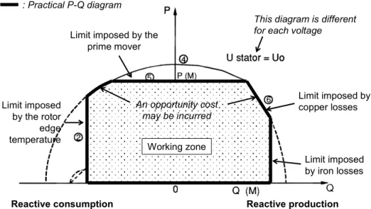
Figure 1.15: Phasor representation associated with Figure 1.14 70 Figure 1.16: Typical P-Q diagram from the stator side. Based on Testud (1991) 73 Figure 1.17: π-representation of a line 74 Figure 1.18: Reactive power consumption of a 400 kV / 2 000 MVA line as a function of

the phase current 76

Figure 2.1: (a) Centralised and (b) decentralised dependent controllers 92 Figure 2.2: The three functional frequency controls considering a generating unit 95 Figure 2.3: Frequency and French regulation signal on 31 March 2005 [Tesseron (2008)] 96 Figure 2.4: The three functional voltage controls considering a generating unit 99 Figure 2.5: Representation of responses of an AS provider for two different inputs 115 Figure 2.6: Classification of AS based on frequency-domain characterisation 116 Figure 2.7: Proposed standardised definition of quality of a frequency or voltage control AS117 Figure 2.8: Representation of the actual response of the group versus its estimate 117 Figure 2.9: Utilisation of a profile to define a category of AS quality 118 Figure 2.10: Deployment of secondary and tertiary controls 123 Figure 2.11: Probability density of the necessary frequency control power 124 Figure 2.12: Empirical and normal cumulative distribution functions of the activated tertiary control power in 2006 in France 126 Figure 2.13: Cost curves of system services 129 Figure 2.14: Allocation of SS costs between four groups of users 131 Figure 2.15: Value of SS for a group of user 131 Figure 2.16: Representation of the optimal quantity q* of SS 132

Figure 2.17: Frequency control reserve indicators in 2004-5 across systems surveyed 135 Figure 2.18: Direct control by the reserve receiving TSO [UCTE (2005)] 139 Figure 2.19: Control through the reserve connecting TSO [UCTE (2005)] 139 Figure 3.1: Representation of two over-sized elements because of voltage control 145 Figure 3.2: Schematic dispatches to understand de-optimisation and opportunity costs 148 Figure 3.3: Overview of the optimisation process at EDF Producer [based on Ernu (2007)]151 Figure 3.4: The two datasets considered to calculate the de-optimisation cost 155

Figure 3.5: APOGEE algorithm 160

Figure 3.6: Principle of OTESS 161

Figure 3.7: Frequency distributions of the gap between APOGEE dispatch and APOGEE demand for all the studied time steps between 1 and 48 164 Figure 3.8: Evolution of the relative de-optimisation cost from 01/01/2005 to 30/08/2007166 Figure 3.9: Frequency distribution of the relative de-optimisation cost for all the studied

days 167 Figure 3.10: Frequency distribution of the variation of de-optimisation cost over two days

for all the studied days 168

Figure 3.11: Autocorrelation function of the de-optimisation cost up to 1-year period 169 Figure 3.12: Partial autocorrelation function of the de-optimisation cost up to 1-year period170 Figure 3.13: Partial autocorrelation function of the de-optimisation cost around a 3-month

period 170 Figure 3.14: Partial autocorrelation function of the de-optimisation cost around a 1-month period 170 Figure 3.15: Partial autocorrelation function of the de-optimisation cost around a 1-week

Figure 3.16: Normalized de-optimisation cost as a function of the average normalized weighted marginal cost of reserves for all the studied days (rxy = 0.94) 172

Figure 3.17: Normalized de-optimisation cost as a function of the average normalized marginal cost of reserves for all the studied days 172 Figure 3.18: Normalized de-optimisation cost as a function of the maximum normalized primary reserve demand for all the studied days (r_xy = 0.39) 174 Figure 3.19: Normalized de-optimisation cost as a function of the maximum normalized primary reserve demand from 01/08/2006 to 31/07/2007 (rxy = 0.71) 174

Figure 3.20: Normalized de-optimisation cost as a function of the maximum normalized primary reserve demand from 01/01/2005 to 31/12/2005 (rxy = 0.13) 174

Figure 3.21: Normalized de-optimisation cost as a function of the mean normalized primary reserve demand for all the studied days (rxy = 0.38) 175

Figure 3.22: Normalized de-optimisation cost as a function of the mean normalized secondary reserve demand for all the studied days (r_xy = -0.18) 175 Figure 3.23: Normalized de-optimisation cost as a function of the minimum reserve share provided by thermal units for all the studied days (rxy = 0.44) 176

Figure 3.24: Relative de-optimisation cost as a function of the new demand for reserve for 24/05/2007 178 Figure 3.25: Simplified relative de-optimisation cost as a function of the new demand for

reserve for 24/05/2007 179

Figure 3.26: Percentage of time when marginal costs of energy are higher than marginal costs of reserves as a function of the time step for all the studied days 180 Figure 3.27: Percentage of time when marginal costs of primary reserve are higher than marginal costs of secondary reserve as a function of the time step for all the studied days 180 Figure 3.28: Percentage of time when marginal costs of reserves are null as a function of the time of the day for all the studied time steps 181

Figure 3.29: Frequency distribution of the relative de-optimisation cost due to time control with ft = 49.99 Hz for all the studied days from 01/01/2005 183

Figure 3.30: Frequency distribution of the relative de-optimisation cost due to time control ft = 50.01 Hz for all the studied days from 01/01/2005 183

Figure 4.1: Impact of the demand responsiveness on market clearing 192 Figure 4.2: NYISO’s demand curve for secondary frequency control. Data based on

NYISO (2008) 193

Figure 4.3: Same utilisation payments for two different utilisations 199 Figure 4.4: Representation of the generic frequency control ancillary service trapezium used in Australia. Based on NEMMCO (2001) 201 Figure 4.5: Reactive power capability curve in Great Britain [National Grid (2008c)] 202 Figure 4.6: Illustration of a gaming possibility with a real-time reactive power market 217 Figure 4.7: Supply curves for different due dates 220 Figure 4.8: Effect of an offer cap (a) and a purchase cap (b) 221 Figure 4.9: Four intensities of an incentive scheme [Keller and Franken (2006)] 232 Figure 4.10: Ancillary services cost indicators across systems surveyed in 2004-5 235 Figure A.1.1: Example of a frequency distribution 294 Figure A.1.2: Schematic representation of the smoothing process 297 Figure A.2.3: Hardware architecture of OTESS 301 Figure A.2.4: Entity relation modelling of the main tables of OTESS 302 Figure A.2.5: Modification and import of datasets with OTESS (operations 2 and 6 in

section A.2.2) 308

253H

Figure A.2.7: Creation of new data in the database (operation 7 in section A.2.2) 309 Figure A.2.8: Basic calculation on the data (operation 7 in section A.2.2) 309 Figure A.2.9: Display of a graph with OTESS (operation 7 in section A.2.2) 310 Figure A.2.10: Analysis of data with OTESS (operation 7 in section A.2.2) 310 ■

17

ABSTRACT

All users of an electrical power system expect that the frequency and voltages

are maintained within acceptable boundaries at all times. Some participants,

mainly generating units, provide the necessary frequency and voltage control

services, called ancillary services. Since these participants are entitled to receive

a payment for the services provided, markets for ancillary services have been

developed along with the liberalisation of electricity markets. However, current

arrangements vary widely from a power system to another.

This thesis provides a comprehensive assessment of markets for

frequency and voltage control ancillary services along three axes: (a) defining

the needs for frequency and voltages, as well as specifying the ancillary services

that can fulfil these needs; (b) assessing the cost of ancillary services for a

producer; and (c) discussing the market design of an efficient procurement of

ancillary services.

Such a comprehensive assessment exhibits several advantages: (a)

stakeholders can quickly grasp the issues related to ancillary services; (b)

participants benefit from a standardised method to assess their system; (c)

solutions are proposed to improve current arrangements; and (d) theoretical

limitations that need future work are identified.

This work, titled A Comprehensive Assessment of Markets for Frequency and

Voltage Control Ancillary Services, was submitted in 2008 by Yann Rebours to

19

DECLARATION

No portion of the work referred to in this thesis has been submitted in support of an application for another degree or qualification of this or any other university or other

21

COPYRIGHT

The author of the thesis (including any appendices and/or schedules to this thesis) owns any copyright in it (the “Copyright”) and s/he has given The University of Manchester the right to use such Copyright for any administrative, promotional, educational and/or teaching purposes.

Copies of this thesis, either in full or in extracts, may be made only in accordance with the regulations of the John Rylands University Library of Manchester. Details of these regulations may be obtained from the Librarian. This page must form part of any such copies made.

The ownership of any patents, designs, trade marks and any and all other intellectual property rights except for the Copyright (the “Intellectual Property Rights”) and any reproductions of copyright works, for example graphs and tables (“Reproductions”), which may be described in this thesis, may not be owned by the author and may be owned by third parties. Such Intellectual Property Rights and Reproductions cannot and must not be made available for use without the prior written permission of the owner(s) of the relevant Intellectual Property Rights and/or Reproductions.

Further information on the conditions under which disclosure, publication and exploitation of this thesis, the Copyright and any Intellectual Property Rights and/or Reproductions described in it may take place is available from the Head of the School of Electrical and Electronic Engineering. ■

23

ACKNOWLEDGEMENT

First, I would like to sincerely thank Pr Daniel Kirschen, who was really an amazing supervisor during these three years. He took the time to discuss and read, had great ideas, made numerous useful comments, showed an open-mindedness and was not bothered by my French accent.

I would also like to thank the people at Electricité de France (EDF) that make this PhD happens, and in particular the persons that got closely involved with this work: Etienne Monnot, Bruno Prestat, Sébastien Rossignol and Marc Trotignon. Moreover, I address particular thanks to Duane Robinson who helped me to find this thesis. Lastly, I would like to thank EDF for its funding over the three years. However, the views expressed in this work are not necessarily those of EDF.

This thesis, though meaning some lonely hard time, matured in an environment both nice and studious. I thus would like to address many thanks to all the fellows from the University of Manchester that helped me enjoy this thesis, and in particular: Chandra for his knowledge of the Curry Mile; Jerry for his pertinent philosophical thoughts; Miguel for his daily quotes from The Simpsons; Ricardo for his enthusiasm to visit the U.K.; Sky for the badminton games; and Vera for the walks in the Peak District. Many thanks also to all my colleagues from EDF, and especially the colourful R12 group, who constantly showed support, suggested ideas and had good cheer. I would like to thank in particular: Sébastien, my first Jedi master; Etienne, who made me run and was constantly of good counsel; Bruno and Méhana, for their support over these three years; Marc, who spent hours reading and discussing the ideas laid in this thesis and others; Stefan, who has always good ideas, especially at Miami Beach or in a squash court; Frédéric, who has unfailingly interesting discussions that pop, from Into the Wild to the amount of wind blowing in Corsica;

Jean-Pierre, with whom we tried to solve the world’s problems (we are still working on it); and Jérôme for his explanations about APOGEE clearer than those about squash.

As it is not possible to find all the information in books, papers or on the Internet, a part of the information given in this thesis come from discussions with various people, in particular: Richard Bénéjean and Jean-Michel Tesseron for historical procedures on frequency control; Jean-Louis Bousquet for transmission lines; Alain Chollois for contracts between landlords and wind producers; Renaud Crinon and Jean-Paul Echivard for the regulation of a nuclear power plant; Arnaud Fauchille for time control; Christian Launay and Romuald Texier-Pauton for EDF’s operational process to dispatch generating units; Virginie Pignon for various subjects in economics; Alain Tanguy for high-voltage transformers; Luc Tran for the behaviour of French hydro units; and François Bouffard and Julián Barquín for their numerous useful comments on the final draft of this thesis. The surveys of the various systems have been possible only with the kind participations of Jürgen Apfelbeck, Christer Bäck, Noel Janssens, Ton Kokkelink, Thomas Meister, Luis Rouco, Ilya Usov and Raymond Vice.

Lastly, I would like to express my thanks to my family and my friends who provide me constant support over these three years and who even got the curiosity to read some of this work. I wish that you keep drying your hair every morning thinking about frequency and voltage controls.

25

ABBREVIATIONS AND

ACRONYMS

AC Alternative Current ACE Area Control Error

ACF AutoCorrelation Function

ADSB Adaptive Deterministic Security Boundaries AER Australian Energy Regulator (Australia) AS Ancillary Service

AU Australia

AVR Automatic Voltage Regulator

BDEW Bundesverband der Energie- und Wasserwirtschaft e.V (Federal association for the energy and water management) (Germany)

BE Belgium

BNA Bundesnetzagentur (regulator of the federal grid) (Germany) CAISO California Independent System Operator (USA)

CAL California

CI Cost Indicator

Cigré Conseil International des Grands Réseaux Electriques (International Council on Large Electric Systems)

CNSE Comisión Nacional del Sistema Eléctrico (National Commission of the Electrical System) (Spain)

CO₂ Carbon dioxide

CPS Control Performance Standard (North America)

CRE Commission de Régulation de l'Energie (Commission of Energy Regulation) (France) CREG Commission de Régulation de l'Electricité et du Gaz (Commission of Electricity and

Gas Regulation) (Belgium) CSV Comma-Separated Values DC Direct Current

DCS Disturbance Control Standard (North America) DE Germany

DG Distributed Generation

DGEMP Direction Générale de l'Energie et des Matières Premières (General Direction of Energy and Raw Materials) (France)

DIDEME DIrection de la DEmande et des Marchés Energétiques (Direction of the Demand and Energy Markets) (France)

DNO Distribution Network Operator DO Distribution Owner DP Dynamic Programming DSO Distribution System Operator

DTe Directie Toezicht Energie (Supervision Department of Energy) (The Netherlands) EDF Electricité de France SA (Electricity of France) (France)

EENS Expected Energy Not Served EnBW EnBW Transportnetze AG (Germany) E.ON E.ON Netz GmbH (Germany)

ERAP Entity Responsible for Ancillary services Procurement

ERCIM European Research Consortium for Informatics and Mathematics (Europe) ES Spain

ETSO European Transmission System Operators (Europe) FACTS Flexible Alternating Current Transmission System FERC Federal Energy Regulatory Commission (USA) FQ First Quartile

FR France FTP File Transfer Protocol FTR Financial Transmission Right GB Great Britain

or Gigabyte

GPS Global Positioning System

HHI Herfindahl-Hirschman Index Hi. High frequency response (Great Britain) HMI Human-Machine Interface

I Intentional or Integral IEA International Energy Agency

IEEE Institute of Electrical and Electronics Engineers IET Institution of Engineering and Technology IMF International Monetary Fund

INPG Institut National Polytechnique de Grenoble (National Polytechnical Institute of Grenoble) (France)

INSTN Institut National des Sciences et Techniques Nucléaires (National Institute of Nuclear Science and Techniques) (France)

IQR InterQuartile Range ISO Independent System Operator KSH Korn Shell

LAMP Linux, Apache, MySQL and PHP

LEG Laboratoire d’Electrotechnique de Grenoble (Electrotechnical Laboratory of Grenoble) (France)

LMP Locational Marginal Price LP Linear Programming LSE Load-Serving Entity (USA) MB Megabyte

MO Market Operator NAG Numerical Algorithms Group

NERC North American Electric Reliability Corporation (North America) NEMMCO National Electricity Market Management Company (Australia) NI Non Intentional

NL The Netherlands NOx Nitrogen Oxide No rec. No recommendation

NYISO New York Independent System Operator (USA) NZ New Zealand

Ofgem Office of Gas and Electricity Markets (Great Britain)

OMEL Operador del Mercado ELéctrico (Electric Market Operator) (Spain) OTC Over-The-Counter

OTESS OuTil pour l’Etude des Services Système (Tool for the study of ancillary services) P Proportional

PACF Partial AutoCorrelation Function PHP PHP: Hypertext Preprocessor PI Proportional Integral PMU Phasor Measurement Unit POD Point of Delivery

Pri. Primary frequency response (Great Britain) PSS Power System Stabilizer

RCT Reserve Connecting TSO (UCTE)

REE Red Eléctrica de España (Spanish Electrical Grid) (Spain) RI Reserve Indicator

RMS Root Mean Square

RRT Reserve Receiving TSO (UCTE) RSI Residual Supply Index

RTE Réseau de Transport d'Electricité (Electrical Transmission Grid) (France) RTO Regional Transmission Organisation (USA)

RWE RWE Transportnetz Strom GmbH (Germany) SE Sweden

Sec. Secondary frequency response (Great Britain) SO System Operator

SO-CDU System Operator-Central Dispatching Upravlenie (Russia) SS System Service

Stem Statens Energimyndighet (Swedish Energy Agency) (Sweden) SVC Static var Compensator

SvK Svenska Kraftnät (Sweden) T Total

TO Transmission Owner TQ Third Quartile

UCEI University of California Energy Institute (USA)

UCPTE Union for the Co-ordination of Production and Transmission of Electricity (Europe)

UCTE Union for the Co-ordination of Transmission of Electricity (Europe) UPFC Unified Power Flow Controller

UPS Unified Power Systems of Russia (Europe and Asia) VCG Vickrey-Clarke-Groves

VET Vattenfall Europe Transmission GmbH (Germany) VOLL Value of Lost Load

33

SYMBOLS

NERC

ACE ACE of zone z according to NERC (in W)

z UCTE

ACE ACE of zone z according to the UCTE (in W) B susceptance of the capacitance (in S)

z

B frequency bias setting of zone z (in W/0.1 Hz) ci cost paid by user i (in €)

C capacitance (in F)

( )

C r cost of the SS deployed (in €)

D

C dispatch cost of the day D (in €)

D on optimisati de

C − de-optimisation cost due to frequency control of the day D (in €)

D h

C hydro dispatch cost of the day D (in €)

D

on optimisati de relative

C − relative de-optimisation cost due to frequency control of the day D (no

unit)

D th

C thermal dispatch cost of the day D (in €)

D reserves with

D reserves without

C dispatch cost while not providing reserves during the day D (in €)

D reserve initial of X with

C % dispatch cost with the demand for reserves equals to X % of the initial

demand of the day D (in €)

z AS

C annual cost of a given ancillary service for zone z (in €/year)

z energy

C annual wholesale energy cost for zone z (in €/year)

z AS

CI cost indicator for a given ancillary service for zone z (no unit) D self-regulation of the load (in %.Hz–1₎

or day (an integer)

DKolmogorov deviation between the empirical F∗(x) and the modelled F(x series, used in )

the Kolmogorov test

z n consumptio

E hourly average energy consumption of the zone z (in MWh/h)

z generation

E hourly average energy production of the zone z (in MWh/h)

) (x₁,x₂...x_n

f objective function (usually in €)

f actual system electrical frequency at the considered point (in Hz)

n

f nominal electrical frequency of the power system (in Hz)

qss

f quasi-steady-state electrical frequency of the power system (in Hz)

t

f target system electrical frequency (in Hz)

i m

f system electrical frequency measured by generating unit i (in Hz)

i n

f the nominal frequency of the power system set in the controller of generating unit i (in Hz)

z m

f system electrical frequency measured by zone z (in Hz) )

(

F x modelled series related to the empirical series F∗(x) )

(

F∗ x empirical series g generating unit number

z

hˆ estimated power deviation of the zone z related to z day max

P (in %) H hour

i current (in A)

or user i in a Groves-Clarke tax system or in the Aumann-Shapley method (integer)

or time step i in APOGEE (integer) I root mean square current (in A)

I complex representation (phasor) of the current (in A) Ibase base current for a given per-unit representation (in A)

I_c characteristic current of a line (in A)

Iconductor maximal permanent current in a line conductor (in A)

Ik complex representation (phasor) of the current flowing in the electrical node k

(in A)

z ME

I factor to compensate the difference between the integration of the instantaneous power exchanged and the demand’s energy measurements of zone z

j constraint number (an integer)

k electrical node

K proportional gain of a first order system (in output unit/input unit)

z

K K-factor of zone z (in W/Hz) L inductance (in H)

or Lagragian function (usually in €) LI Lerner index (no unit)

n number of variables to optimise (an integer) ni net value got by the user i (in €)

N_G number of generating units providing speed control p instantaneous power (in VA)

pm number of poles of an electrical rotating machine

pr instantaneous active power (in W)

px instantaneous reactive power (in var)

P_consumption total active power consumed in the power system (in W)

z n consumptio

Pˆ estimate of the internal consumption of the zone z (in MW)

z

n consumptio max

Pˆ estimate of the maximal internal consumption of the zone z (in MW) P average instantaneous active power or simply active power (in W) P complex representation (phasor) of the active power (in W)

P0 electrical active power consumed and produced before the perturbation (in W)

Pe electrical active power (in W)

P_k active power flowing through the electrical node k (in W) Pl power loses in the process (in W)

Pm mechanical active power sent to an electrical rotating machine (in W)

Pn nominal active power produced by the generating unit (in W) i

demand

P demand for power generation for the time step i (in MW)

i dispatch

P power generation dispatched during the time step i (in MW)

i G0

P active power set-point of the generating unit i without any frequency control (in W)

i Gn

P nominal output active power of the generating unit i (in W)

z ction interconne

P active power exported by the zone z to the power system (in W)

z 0 ction interconne

P scheduled active power exported by the zone z to the power system (in W)

z

m ction interconne

P measured value of the total power exchanged by the zone with other zones, where a positive value represents exports (in W)

z generation max

Pˆ estimate of the peak generation for the zone z for the day (in MW) PC price cap (in €/MW)

i P

Penalty penalty due to the power mismatch for the time step i (in €)

i Rpri

Penalty penalty due to the primary frequency control reserve mismatch for the time step i (in €)

i Rsec

Penalty penalty due to the secondary frequency control reserve mismatch for the time

step i (in €)

q* clearing quantity (in good unit)

∗

qr quantities of SS actually used (e.g., in MWh)

i

q quantity of SS actually used by user i (e.g., in MWh)

Q maximum of the instantaneous reactive power or simply the reactive power (in var)

Q complex representation (phasor) of the reactive power (in var) Qk reactive power flowing through the electrical node k (in var)

Qn nominal reactive power produced by the generating unit (in var)

Q_POD reactive power flowing through the point of delivery (in var) rxy cross-correlation between two series (no unit)

R resistance (in Ω)

z pri

R primary frequency control reserve of the zone z (in MW)

i demand pri

R demand for primary frequency control reserve for the time step i (in MW)

i dispatch pri

R primary frequency control reserve dispatched during the time step i (in MW)

i th dispatch pri

R primary frequency control reserve dispatched on thermal units during the time step i (in MW)

z sec

R secondary frequency control reserve of the zone z (in MW)

i demand sec

R demand for secondary frequency control reserve for the time step i (in MW)

i dispatch sec

R secondary frequency control reserve dispatched during the time step i (in MW)

i th dispatch sec

R secondary frequency control reserve dispatched on thermal units during the time step i (in MW)

z pri

RI reserve indicator for the primary frequency control reserve of the zone z (in %)

z sec

RI reserve indicator for the secondary frequency control reserve of the zone z (in %)

S apparent power (in VA)

S complex representation (phasor) of the apparent power (in VA) S_base base apparent power for a given per-unit representation (in VA) Sline apparent power admissible by the line (in VA)

Sn nominal apparent power produced by an electrical machine (in VA) i

G

s droop of the generating unit i (in per-unit)

i th

share thermal reserve share for time step i (no unit) t time (in s)

a deployment

t deployment time a (in s)

b deployment

t deployment time b (in s) T cycle time (in s)

or time constant of a first order system (in s) Te electrical torque (in N.m)

T_m mechanical torque exercised on the rotor of an electrical rotating machine (in N.m)

u voltage across a dipole (in V)

U root mean square voltage of u (in V) Udim network dimensioning voltage (in V)

U_n network nominal voltage (in V) vi value put by the user i (in €)

V average voltage between two electrical nodes (in V) Vbase base voltage for a given per-unit representation (in V)

Vk root mean square voltage from the ground to the electrical node k (in V)

V_k complex representation (phasor) of the voltage from the ground to the electrical node k (in V)

Vline-line the voltage line-to-line of the line (in V)

) (

ω_j x₁,x₂...x_n constraint function (in various units)

window the width of the extrapolation (an odd integer larger or equal to three) x data of the temporal series (in series’ unit)

ed extrapolat

x extrapolated data to complete the temporal series (in series’ unit)

n

x primal variable to optimise (various units) X reactance of an inductance (in Ω)

or the amount of the initial demand for reserves (in %) z power system zone number (integer)

Z impedance (in Ω)

base

Z base impedance for a given per-unit representation (in Ω)

c

Z characteristic impedance of a line (in Ω) δ angle between two voltages (in rad) ε accuracy of measurement (in % or in Hz)

D on optimisati de

C −

Δ% relative variation of the de-optimisation cost for D in comparison to D–1 (no unit)

f

Δ quasi-steady-sate frequency deviation from the nominal frequency fn (in Hz) i

m

f

Δ measured frequency deviation by the generating unit i (in Hz) P

Δ quasi-steady-state power unbalance

n consumptio

P

Δ consumption change following a quasi-steady-sate frequency deviation (in W)

generation

P

Δ generation change following a quasi-steady-sate frequency deviation (in W)

i G

P

Δ change in the active power set-point of the generating unit i for any frequency deviation (in W)

z n consumptio

P

Δ consumption change in zone z following a quasi-steady-sate frequency deviation (in W)

z generation

P

Δ generation change in zone z following a quasi-steady-sate frequency deviation (in W)

z ction interconne

P

Δ change in the power transfer between the zone and the other interconnected power systems (in W)

V

Δ voltage difference between two electrical nodes (in V) ϕ lag between current and voltage (in rad)

λ instantaneous frequency characteristic (in W/Hz)

j

λ Lagrange multiplier related to the constraint j (usually in €/unit of the constraint)

i P

λ marginal cost of power for the time step i (in €/MWh)

i R

i Rpri

λ marginal cost of primary frequency control reserves for the time step i (in (€/MW)/h)

i Rsec

λ marginal cost of secondary frequency control reserves for the time step i (in (€/MW)/h)

Λ frequency characteristic of the power system for a given frequency deviation (in W/Hz)

z

Λ frequency characteristic of the zone z for a given frequency deviation (in MW/Hz)

∗

π clearing price (in currency unit/good unit)

π

~ _{simulated competitive price (in currency unit/good unit)}

i

π price paid by user i (in €/MW)

σ standard deviation (in the unit of the value considered) τ delay (in s)

ω electrical angular frequency (in rad.s–1₎

m

A Comprehensive Assessment of Markets for Frequency and Voltage Control Ancillary Services, Yann Rebours, 2008 43

CHAPTER 1

Chapter 1

INTRODUCTION

Never be entirely idle; but either be reading, or writing, or praying or meditating or endeavouring something for the public good. Thomas a Kempis (1380 - 1471)

1.1 Increasing Welfare of Power System Users

USER connected to a power system (e.g., a generating unit or a consumer) wishes to have access to a system that meets a certain standard of quality. In particular, this user expects that the frequency and voltage will stay close to their nominal values because most electrical appliances are designed for a particular frequency and a given voltage. Failure to meet these frequency and voltage standards would lead to losses for the users that may range from a burnt bulb to the loss of production in an expensive process (e.g., in an automobile factory). Efficient frequency and voltage controls are thus essential to maintain a high welfare for all power system users.

The frequency and voltage control services are called system services (SS) because they are delivered by the power system to all the users. Some users of the system, such as generators, contribute to these system services by acting on the frequency of the system or the voltage at the point where they are connected to the system. Because these services

provided by users are ancillary to the production or consumption of energy, they are called ancillary services (AS). This distinction between system and ancillary services is depicted in Figure 1.1.

Power system

Ancillary services

System services

(e.g., frequency and voltage controls) Some users

(e.g., generators) The other users

Figure 1.1: Distinction between ancillary and system services. Based on Eurelectric (2000)

Ancillary services have been provided by users of the power system since its early days, more than one hundred years ago. However, it is only since the recent liberalization of the electricity sector that ancillary services have been treated as a commodity by themselves. Indeed, the reform of the electricity sector has led to a separation between network and generation activities (see section 1.2). Markets for ancillary services resulting from this separation have been developed independently across countries, depending on the previous historical procedures or market architecture. Markets for ancillary services are thus currently very different across systems. In addition, while ancillary services are commodities that differ in many ways from the electrical energy product, efforts in the liberalization process were concentrated on the main product, i.e. electrical energy and its transmission. Therefore, the theoretical framework is much less advanced for ancillary services than it is for energy and transmission markets. Lastly, the structure of power systems is currently evolving fast, driven by high energy prices, aging infrastructures, increasing environmental constraints, an intensified competition and the appearance of new technologies. For example, new generation technologies are developed, interconnections between countries are used closer to their limit and consumers are getting more active. Hence, markets for ancillary services have to be adapted to this evolving structure.

In summary, markets for ancillary services are disparate across countries; they lack from a consistent theoretical framework; and they have to be constantly adapted to the changing structure of power systems. It is thus essential to assess current markets for ancillary services to avoid inappropriate architectures that would lead to inefficiencies and thus a reduced global welfare. However, stakeholders do not have a general and systematic

tool that would help them assess the current markets for ancillary services and thus improve current practices. Therefore, this thesis proposes to fill this gap by providing the tools to perform a comprehensive assessment of markets for ancillary services along three aspects: the technical definition of ancillary services, the cost of provision and the market design.

First, contrary to previous works that were concentrated on specific aspects of markets for ancillary services, this thesis gives a complete picture of the issues by developing the technique, the cost and the market design together. Indeed, these three aspects are linked. For example, the technical definition of an ancillary service will have an impact on the cost to provide it (e.g., a more complex service is likely to be more expensive to provide than a simpler one); the cost structure influences the market design (e.g., a cost that is constant over time makes a short-term market unnecessary); and the technical characteristics of an ancillary service may not be suitable for some particular market design (e.g., it is useless to build a market over a large geographical area if a product is useful only in a given power system region).

Second, the proposed assessment is based on a framework that can be applied to any system. This framework is developed as follows: (a) identifying features; (b) expressing the issues related to each feature; (c) describing the actual solutions adopted in various systems across the world; (d) proposing innovative solutions. Therefore, both theoretical and practical aspects are tackled. At the end of each core chapter, an assessment checklist is proposed to help stakeholders improve their system by implementing new solutions or by fostering more research on a specific feature. Indeed, by putting together issues and solutions for each feature, a global solution to manage ancillary services becomes much clearer.

This thesis is organised in five chapters. Chapter 1 presents the basic layout, the stakeholders and the marketplaces of a power system. The basic concepts underlying frequency and voltage controls are then introduced. Even if this thesis is focused on the ancillary services provided by conventional large generating units, most of the concepts are applicable to any provider of ancillary services as well. The explanations are intended to be suitable for all readers irrespective of their technical background. In particular, the concept of reactive power is explained. Nevertheless, readers familiar with frequency control will notice that the new concepts of average and instantaneous frequency characteristics are defined. Lastly, technologies providing ancillary services are presented.

Chapter 2 focuses on the delivery of ancillary services. First, the needs of users in terms of system services are examined. To meet these needs, ancillary services have to be provided by some users of the system. Therefore, the specification of the quality of ancillary services is discussed. Lastly, the optimal quantity and location of the ancillary services are debated. In particular, Chapter 2 shows that the amount of ancillary services currently provided does not correspond to the actual needs of users in terms of system services.

Chapter 3 describes the main costs incurred by the provision of ancillary services by a producer. A practical methodology to evaluate the cost of frequency control due to the day-ahead capacity reservation is then proposed and successfully applied to Electricité de France (EDF) Producer’s portfolio. In particular, this study gives interesting insights on the parameters affecting the cost of frequency control. Lastly, the cost of the time control (i.e., the cost to maintain the frequency average at 50 Hz) is assessed for France.

Chapter 4 reviews the numerous issues related to the procurement of ancillary services, namely: (a) nominating the responsible entity of procurement; (b) matching supply and demand; (c) choosing the relevant procurement method; (d) defining the structures of offers and payments; (e) organizing the market clearing procedure; (f) avoiding price caps; (g) providing appropriate incentives; (h) assessing the procurement method. Practical and innovative solutions are proposed for each issue.

Lastly, Chapter 5 provides a summary of this thesis, some scenarios of evolutions and possible future work.

1.2 Stakeholders

Broadly speaking, the elements of a power system are physically divided into three main categories: generating units, the network and loads. The network, which provides the electrical link between loads and generating units, is actually divided into two main parts (see Figure 1.2). The transmission network is meshed and operated at high voltages (e.g., 63 kV to 400 kV in France), while the distribution network is usually operated in a radial fashion and at lower voltages (e.g., 400 V to 20 kV in France). Networks are mainly constituted of lines,

transformers1 _{and various controllers. Conventional large generation (e.g., coal, nuclear, large}

hydro, gas or fuel) are connected to the transmission network, while smaller generation (e.g., wind, small hydro, combined heat-power plant or photovoltaic) tend to be connected to the distribution network, which led to the term of distributed generation (DG) to designate this kind of generating units. Lastly, consumers withdraw energy from the system, either at the transmission level (large consumers) or at the distribution level (small consumers).

The various elements of a power system are owned by different parties. Prior to liberalisation, most of them were owned by vertically-integrated companies, which owned at the same time generation, transmission, distribution and retail. Currently, the ownership of these activities tends to be separated. Large generating units are owned by generation companies, which most of the time finds their roots in the historical vertically-integrated companies. The transmission network is owned by a few entities (Transmission Owners, TO, or transmission companies), whereas distribution networks are usually owned by many entities (Distribution Owners, DO, or distribution companies), such as the city councils in France. Lastly, end users are obviously owned by a large number of stakeholders. Therefore, end users are usually gathered in consumer associations to get a more powerful representation. In addition, they deal with retailers (or suppliers), which buy large volumes of energy from generation companies and is in relation with the intermediate stakeholders, such as distribution and transmission operators. In certain cases, retailers can also buy the electricity produced by the end users who own generating assets. Note that retailers generally do not own significant physical assets, except intelligent meters in some cases.

A liberalised power system is complex to run because of the number of participants involved. In addition, it has been recognized that the operation of electrical networks is a natural monopoly. Therefore, independent bodies have to be designated to manage the power system (the system operators, or SO). The Transmission System Operator (TSO) operates the power system at the transmission level, while the Distribution System Operator (DSO) is in charge of the distribution level. Therefore, from the TSO’s perspective, a DSO is equivalent to a large consumer. Note that the terms Distribution Network Operator

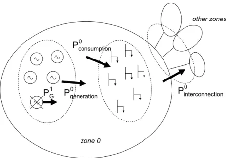
1 _{A transformer allows to converts energy from a given voltage to another level with the help of two}

windings around a magnetic circuit. The first winding brings power into the magnetic circuit, while the second winding withdraws power from it. A difference in the number of turns for each winding leads to a voltage change, but with a similar power transmitted. Note that Figure 1.2 did not explicitly display any transformers.

(DNO), Regional Transmission Organisation (RTO) and Independent System Operator (ISO) can also be found, with responsibility and authority varying amongst systems.

The competitive sectors of the electricity industry, i.e. generation and retail, need marketplaces to trade products (see next section). The Market Operators (MO) are in charge of these marketplaces. In addition, other participants may provide additional services in the marketplace, such as the brokers, who help bring buyers and sellers together.

To foster fair relations between stakeholders, three basic functions should be performed: (a) setting the rules; (b) monitoring that the rules are respected; and (c) enforcing the rules if necessary. Arrangements to perform these three functions vary from one system to another. The rules are usually set by the legislator, which is most of the time the legislative body of the government. The regulator, which is independent, then checks whether the rules are respected by the participants. It also collects complaints from stakeholders. It may also propose some rule modifications to the legislator. Lastly, it oversees the quality of services provided by participants. Depending on the countries considered, the power of regulators to enforce rules varies. Some of these powers may be entrusted to other entities, such as an anti-trust commission or a market monitoring entity.

Frequency and voltage controls involve all the stakeholders described above. Indeed, generation companies, system operators and end users modify the frequency and voltages through their actions, as explained in Chapters 1 and 2. In addition, the market operators, the regulator and the legislator design the rules used to manage frequency and voltage controls, as shown in Chapters 2 and 4.

Small consumer Transmission network Distribution network

~

~

Figure 1.2: Basic layout of a power system

1.3 Marketplaces

In order to facilitate exchanges of products between stakeholders and to send signals to all the participants, markets have been developed along with the liberalization. Section 1.3.1 presents the basic features of a marketplace, while sections 1.3.2 to 1.3.5 introduce the main marketplaces that one is likely to find in the electrical industry.

1.3.1 Basic features of a marketplace

The goal of a marketplace is to bring a buyer and a seller together, so they can exchange a given good at an agreed price. If the delivery of the good is instantaneous (e.g., when one buys some Camembert cheese at a favourite dairy shop), or if the good cannot be resold by the buyer before the delivery (e.g., when one buys a Norman wardrobe to be delivered to the buyer the next day), the market is called a spot market. Otherwise, the quality of the good has to be described, as well as the date of delivery and the price to be paid at delivery. Such a market where commodities are traded for delivery in the future is named futures (or sometimes forward) market. In practice, there are several futures markets, which deal with a particular product (e.g., 1-year or 6-month delivery). Obviously, the products of the 1-year futures market can be traded 6 month later in the 6-month futures market. Futures markets

are useful to participants to hedge against risk associated with the volatility of the spot prices.

To trade these products (spot or future), the marketplace can be organised in two ways. A centralised market is cleared by a unique entity that collects the offers to sell (supply curve) and the bids to buy (demand curve). A unique price π* is seen by both buyers and sellers, and a quantity q* is traded. This price and this quantity correspond to the point where supply and demand match (see Figure 1.3). Note that it can be easily proven that the price π* is equal to the marginal cost of the producer2 _{providing the last offer (considering a}

perfectly competitive market3_{). On the other hand, in a decentralised market, sellers and buyers}

can enter directly into contracts to buy and sell (sometimes without knowing each other’s identity). The transaction is thus bilateral. In such a market, there is no “official price”, but there may be mechanisms that allow all the participants to be informed of either the price of the last trade or a weighted average of recent transactions.

An important feature of a marketplace is liquidity. Market liquidity characterises the market’s ability to quickly match any bid to buy with an offer to sell without changing the market price. The liquidity incorporates four features: the tightness (i.e., the capability to avoid a large spread between the highest demand price and the lowest supply price); the depth (i.e., the capability to absorb large trade volumes without significant price changes); the immediacy (i.e., the capability to quickly meet the demand to sell or buy); and the resilience (i.e., the capability to recover after a price change) [IMF (2006)].

The participants can also decide not to meet in a public marketplace, but to agree on a bilateral contract outside any organised structure. This kind of transaction, which is very popular in the electricity industry to manage long-term contracts, is called over-the-counter (OTC)4_{. Such transactions are usually facilitated by brokers. If the bilateral contract is firm,}

it is called a forward contract. On the other hand, if the delivery is optional, it is called an option. Several types of options are possible: European (a unique date of delivery), American (which can be exercised once before a given date), swing (which can be exercised several

2 _{The marginal cost is the cost to provide an additional good in the delivery (one MWh in the case of}

an energy market).

3 _{A perfect competitive market is a market where no participant uses its dominant position to distort}

the signals sent by the market to participants.

4 _{On the down side, OTC contracts cannot guarantee the product provision, whereas the market}

times, but there is a limit in terms of energy), Asian (which is a variant of European: the average price of the good is taken instead of the spot price) or Bermuda (which can be exercised at some given dates). Kluge (2006) describes in depth methods to price options in electricity markets.

Both organised and OTC markets lead to an equilibrium, i.e. a set of operations by stakeholders that equals supply and demand. This equilibrium can be either Pareto efficient, i.e. it is impossible to increase the benefit of a party without decreasing the benefit of the others, or qualified as a Nash equilibrium, i.e. in which no participant has interest to change its position. Note that a Pareto equilibrium takes into account potential cooperative behaviours by stakeholders, whereas a Nash equilibrium is obtained only with the help of unilateral decisions. Therefore, a Nash equilibrium is often not Pareto efficient.

Kirschen and Strbac (2004a) provide a comprehensive introduction to the marketplaces in the electrical industry. Varian (1999) gives a more general and more theoretical view on marketplaces. Furthermore, Chapter 4 is dedicated to the design of a marketplace for ancillary services.

Demand quantity price Supply q* π*

Figure 1.3: Market equilibrium

1.3.2 Generation markets

Generation markets help generation companies find buyers for their products, i.e. energy and ancillary services. Because generating units have a large investment cost, may require a long building period (e.g., around ten years to design a nuclear power plant and up to seven years to build it) and have lifetimes that usually span over tens of years, generation

companies need to find buyers for their products over a long period to reduce risks. In particular, sufficient revenues are essential for generation companies to invest and thus to maintain sufficient capacity in the long-run5_{. Therefore, long-term markets are essential in}

generation markets. In practice, the generation companies secure their investment with long-term OTC bilateral contracts or vertical integration. However, futures markets in electricity are deemed to provide unreliable signals. In fact, the price of futures tends to be constant whatever is the delivery date (e.g., 1-year, 2-year or 3-year delivery) [e.g., Powernext (2008)], whereas the price of electricity is likely to increase in the future. Therefore, long-term generation markets are still an issue in electricity markets.

Once the generating units have been built and most of the power traded in an OTC manner, generation companies and the buyers of their products enter in the short-term futures markets (i.e., one-month or shorter) to balance their positions. Finally, the market closest to real-time is the spot market. This spot market can be organised either with a centralised (pool) or a decentralised (exchange) unit commitment, as discussed in section 4.6.1. If the delivery delay of the spot market is too long (e.g., more than 15 minutes), an additional market is necessary to balance the positions of the participants. This additional market is called the balancing mechanism (or balancing market). This kind of market is more restrictive than the day-ahead market6 _{in order to avoid the exercise of}

market power by some participants (e.g., prices cannot be changed easily) and is usually operated by the system operator.

Markets for ancillary services, which are described in depth in Chapter 4, are part of the generation markets. In particular, markets for ancillary services and for energy are tightly linked, since a generation company can make the choice to allocate one MW of production capacity as an ancillary service or as energy.

For further information on generation markets, see for example Wilson (2002), Kirschen and Strbac (2004a), Baldick et al. (2005) or Joskow (2006). DGEMP/DIDEME (2003) provides reference prices for generating plants, as well as their building time.

5 _{Building sufficient generating capacity in the long-term is part of the power system adequacy issue}

described in section 2.2.1.

1.3.3 Transmission markets

To allow sellers and buyers to trade in the generation markets, a transmission network is necessary. Such a network exhibits some particularities. First, electricity follows physics and not the financial rules, so the impact of an injection or a withdrawal of electrical power does not have necessarily a logical consequence from a business point of view (e.g., an increase in electrical power consumption can reduce the price of this power). Second, it is difficult to build competing transmission lines, so the access to the transmission network has to be managed by an independent entity (the TSO)7_.

Since the transmission network has a cost, participants have to pay for the right to use it. To charge users, Transmission System Operators rely on two methods. First, they can charge the users with an ex-ante price, i.e. the users know in advance the price that they are going to pay for their transmission use. A typical example of an ex-ante price is the postage stamp, for which the users pay a transmission fee that does not depend on the location of the energy generation or consumption. This tariff is designed to recover the cost of transmission expansion and operation, but the signals sent to participants may be too weak to foster an optimal use of the transmission network (e.g., to encourage the construction of new generation plants in a congested area). On the other hand, an ex-post price is possible. Such a price is calculated after (and not prior) the actual use of the network. To allow hedging, some ex-post price estimates are given to the participants. Ex-post prices are often used for competitive procurements of the available transmission capacity. However, the actual implementation of such competitive procurements is still under debate. A popular approach in USA is to link transmission and generation markets by defining energy prices at each node of the system. Such prices are called Locational Marginal Prices (LMP) and are precisely computed ex-post. The differences between the LMPs then provide an income to the owner of the line between the two nodes. Such nodal energy markets are completed with financial instruments that allow a party to hedge against price differences between two nodes of the network (the Financial Transmission Rights, or FTR). Quintana and Bautista (2006) give a short and comprehensible introduction to this topic.

7 _{However, the actual construction of the lines may be done by entities under competition (the}