Planning renewal of water mains while considering deterioration, economies of scale and adjacent infrastructure

Publisher’s version / Version de l'éditeur:

Vous avez des questions? Nous pouvons vous aider. Pour communiquer directement avec un auteur, consultez la

première page de la revue dans laquelle son article a été publié afin de trouver ses coordonnées. Si vous n’arrivez pas à les repérer, communiquez avec nous à PublicationsArchive-ArchivesPublications@nrc-cnrc.gc.ca.

Questions? Contact the NRC Publications Archive team at

PublicationsArchive-ArchivesPublications@nrc-cnrc.gc.ca. If you wish to email the authors directly, please see the first page of the publication for their contact information.

https://publications-cnrc.canada.ca/fra/droits

L’accès à ce site Web et l’utilisation de son contenu sont assujettis aux conditions présentées dans le site

LISEZ CES CONDITIONS ATTENTIVEMENT AVANT D’UTILISER CE SITE WEB.

Proceedings of the 2nd International Conference on Water Economics, Statistics and Finance, IWA Specialist Group Statistics and Economics: 03 July 2009, Alexandroupolis, Greece, pp. 1-13, 2009-07-03

READ THESE TERMS AND CONDITIONS CAREFULLY BEFORE USING THIS WEBSITE.

https://nrc-publications.canada.ca/eng/copyright

NRC Publications Archive Record / Notice des Archives des publications du CNRC :

https://nrc-publications.canada.ca/eng/view/object/?id=ef7f57a1-24ee-4903-b697-422fde58e7d5 https://publications-cnrc.canada.ca/fra/voir/objet/?id=ef7f57a1-24ee-4903-b697-422fde58e7d5

NRC Publications Archive

Archives des publications du CNRC

This publication could be one of several versions: author’s original, accepted manuscript or the publisher’s version. / La version de cette publication peut être l’une des suivantes : la version prépublication de l’auteur, la version acceptée du manuscrit ou la version de l’éditeur.

Access and use of this website and the material on it are subject to the Terms and Conditions set forth at

Planning renewal of water mains while considering deterioration, economies of scale and adjacent infrastructure

http://www.nrc-cnrc.gc.ca/irc

Pla nning re ne w a l of w a t e r m a ins w hile c onside ring de t e riora t ion, e c onom ie s of sc a le a nd a dja c e nt infra st ruc t ure

N R C C - 5 1 4 1 1

K l e i n e r , Y . ; N a f i , A . ; R a j a n i , B . B .

J u l y 2 0 0 9

A version of this document is published in / Une version de ce document se trouve dans:

Proceedings 2nd International Conference on Water Economics, Statistics and Finance, IWA Specialist Group Statistics and Economics (Alexandroupolis, Greece, July 03, 2009), pp. 1-13

The material in this document is covered by the provisions of the Copyright Act, by Canadian laws, policies, regulations and international agreements. Such provisions serve to identify the information source and, in specific instances, to prohibit reproduction of materials without written permission. For more information visit http://laws.justice.gc.ca/en/showtdm/cs/C-42

Les renseignements dans ce document sont protégés par la Loi sur le droit d'auteur, par les lois, les politiques et les règlements du Canada et des accords internationaux. Ces dispositions permettent d'identifier la source de l'information et, dans certains cas, d'interdire la copie de documents sans permission écrite. Pour obtenir de plus amples renseignements : http://lois.justice.gc.ca/fr/showtdm/cs/C-42

Planning renewal of water mains while considering deterioration,

economies of scale and adjacent infrastructure

Yehuda Kleiner1, Amir Nafi2 and Balvant Rajani1

1. National Research Council of Canada, Institute for Research in Construction, Ottawa, Canada. 2. Joint Research Unit in Public Utilities Management, Cemagref-Engees, Strasbourg, France.

Abstract

The structural deterioration of water mains and their subsequent failure are affected by many factors, both static (e.g., pipe material, pipe size, age (vintage), soil type) and dynamic (e.g., climate, cathodic protection, pressure zone changes). This paper

describes a non-homogeneous Poisson model developed for the analysis and forecast of breakage patterns in individual water mains, while considering both static and dynamic factors. Subsequently, these forecasted breakage patterns are used to schedule the renewal of water mains in an economically efficient manner, while considering the various associated costs, including economies of scale and scheduled works on adjacent infrastructure.

In this paper, his principles of the approach are described briefly and its application is demonstrated with the help of a case study.

1. Introduction

The statistical analysis of historical breakage patterns of water mains is a cost effective approach to discern their deterioration, where physical mechanisms that lead to their deterioration are often very complex and not well understood. Furthermore, enormous variability exists in all the factors that contribute to pipe deterioration, and the data required to model these physical mechanisms are rarely available and prohibitively costly to acquire.

Many models have been proposed to discern historical breakage patterns and forecast anticipated future breakage rates. Kleiner and Rajani, (2001) provided a comprehensive review of approaches and methods that had been developed. Since then, several more methods have been proposed, such as Park and Loganathan (2002), Mailhot et al. (2003), Dridi et al. (2005), Giustolisi et al. (2005), Watson et al. (2006), Boxall et al. (2007) and Le Gat (2007) to name but a few.

Kleiner and Rajani (2008) proposed an approach based on the assumption that breaks on an individual pipe occur as a non-homogeneous Poisson process (NHPP). NHPP has been suggested by others to model the same phenomenon (e.g., Constantine and

Darroch, 1993; Røstum, 2000; Jarrett et al., 2003, among others). However, these considered only static factors (i.e., pipe-intrinsic), while the approach proposed Kleiner and Rajani (2008) allowed for the consideration of dynamic factors as well. The NHPP-based model, with time-dependent (dynamic) covariates was named I-WARP

Given a forecast of anticipated future breaks, Nafi and Kleiner (2009) proposed a method for the optimal scheduling of individual pipes for replacement, while considering practical issues such as harmonizing pipe replacement with known scheduled roadwork and economies of scale. Although this method is not restricted to any planning horizon length, it is deemed most suitable for short to mid-term planning (say, 5 years) due to practical considerations such as municipal budgetary planning horizon, confidence (or rather lack thereof) in longer term forecasting of breakage rates in individual water mains and likelihood of unforeseeable changing conditions.

In this paper we provide a brief introduction of the NHPP-based deterioration model (I-WARP) and the renewal scheduling model and demonstrate their application using a case study.

2. Non homogeneous Poisson-based model

In I-WARP we assume that breaks at year t for an individual pipe i are Poisson arrivals with mean intensity (or mean rate of occurrence) λi,t. Therefore, the probability of

observing ki,t breaks is given by:

! ) exp( ) ( , , , , , t i t i k t i t i k k P t i λ λ ⋅ − = where _, exp[ ( _, ) i t i,t] t i o t i α θτ g αz βp γq λ = + + + + (1)

where αo is a constant, τ( gi,t) is the age covariate, and θ is its coefficient, gi,t is the age

of pipe i at year t; zi is a row vector of pipe-dependent covariates (e.g., length, diameter, etc.) and α is a column vector of the corresponding coefficients; pt is a row vector of time-dependent covariates (e.g., climate) and β is a column vector of the corresponding coefficients; qi,tis a row vector of both pipe-dependent and time-dependent covariates (e.g., number of known previous failures - NOKPF, cathodic protection) and γ is a column vector of the corresponding coefficients. We call the function exp[θτ(gi,t)]

“ageing function” and therefore coefficient θ is called “ageing coefficient”. Note that if

τ(gi,t) = gi,t then the aging is exponential, i.e., λ is an exponential function of pipe age,

whereas if τ(t) = loge(gi,t) the aging function becomes a power function, i.e., λ becomes

a power function of pipe age. Year t is taken relative to the first year for which breakage records are available. Coefficients are found by the maximum likelihood method. Note that this formulation implies that each covariate affects the mean intensity independently, i.e., interdependencies between covariates are assumed non-existent, unless a specific covariate is constructed to explicitly consider such interdependency (e.g., a ratio or a product of two “independent” covariates).

3. Covariates

The selection of covariates is obviously limited by the amount and quality of available data. Further, subject to fundamental assumptions, most pipe-dependent covariates (e.g., pipe material, vintage, etc.) can be considered explicitly in the probabilistic model or implicitly by partitioning the data into homogeneous populations with respect to

these covariates. Kleiner and Rajani (2008) discussed at some length the implications as well as the pros and cons of the two approaches for considering these covariates. In this paper, with one exception, we used the latter, i.e., we applied I-WARP to

‘homogeneous’ groups of pipes. The exception is the pipe length covariate, which is considered explicitly.

In the category of time-dependent covariates, three climate-related covariates are considered, namely freezing index (FI), cumulative rain deficit (RDc) and snapshot rain deficit (RDs). A detailed introduction and a rational for using these covariates are provided in Kleiner and Rajani (2004). FI is a surrogate for the severity of a winter,

RDc is a surrogate for average annual soil moisture and RDs is a surrogate for locked-in winter soil moisture (appropriate for cold regions, where soil/backfill can freeze in the winter). Note that climate-related covariates can be used to train the model on observed historical breaks but not to forecast (unless one endeavours to forecast climate as well). The rational for using climate-related covariates is that “true” background ageing rate (in terms of increase in breakage intensity as a function of time) are more likely to emerge if external effects, such as climate, are considered in the training process. In the pipe and time-dependent category two pipe-dependent and time-dependent covariates are considered, namely number of known previous failures (NOKPF) and a covariate related to hotspot cathodic protection (HSCP).

The dependency of pipe failure rate on the number of previous failures has been observed by others (e.g., Andreou et al., 1987; Rostum, 2000). Typically, covariates used have been break order, or number of breaks observed since installation. As the vast majority of water utilities do not have a complete breakage history of pipes since installation (left censored data), a more realistically available (if less rigorous) covariate of previously known number of failures was selected.

There are generally two types of cathodic protection (CP) for water mains, retrofit and hotspot (HSCP). While retrofit CP is the systematic installation of sacrificial anodes along the pipe (or in anode beds), HSCP is the opportunistic placement of a sacrificial anode every time a pipe is exposed for repair. Kleiner and Rajani (2008) described the manner with which the HSCP covariate is computed and considered. The model does allow for the consideration of retrofit CP, but details are yet to be published in a forthcoming AwwaRF report. The case study presented here includes no retrofitted pipes.

4. The economics of pipe replacement

The present value of the total cost associated with pipe i, which is replaced at year t is given by

∑

₊

₊

₊

₊

₊

=

CR

e

k

C

C

C

e

C

C

C

[(

)

]

where CRi,t is the cost of replacing pipe i at year t, e-rt is the exponential form of

t, Cirep the cost of failure repair, Cidir is the cost of expected direct damage (e.g., to

adjacent infrastructure, basement flooding, road damage), Ciindir is the cost of indirect

damage (e.g., accelerated deterioration of roads, sewers, etc.), Ciwat is the cost of loss

water, and Cisoc is the social cost (e.g., disruption, time loss, pollution, loss of business,

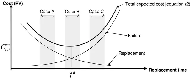
etc.). Note that the indirect cost and social cost components of pipe failure are not discounted. Note further that for public projects such as water main works it is appropriate to use “social discount rate”, which is significantly lower (typically 1% - 3%) than financial discount rate. Equation (2) also implies that the number of failure expected to occur on the new replacement pipe during the planning period T is negligible. This implication is justified for relatively short planning periods. The literature reflects (e.g., Shamir and Howard, 1979; Kleiner et al. 1998) that equation (2) generally describes a convex present value cost function as illustrated in Figure 1. Herz (1999) agreed that the cost function is generally convex but observed that often it is very flat, especially in the inclining branch (the right side) of the curve, creating a “hammock” shaped function. The point of minimum cost of pipe i (ti*) is the point at which the marginal (discounted) cumulative cost of failure rate, which is essentially the expected (discounted) cost of failure at year ti* equals the marginal

savings due to deferral of replacement.

Replacement time

Total expected cost [equation (2)]

tot t i

C

t*

Figure 1. Costs associated with replacement timing

Based on the assumptions about the shape and properties of equation (2), the following three cases are understood for some planning period T:

1. T is located to the left of ti* (i.e., case A in Figure 1)

2. T coincides with ti* (i.e., case B in Figure 1).

3. T is located to right of ti* (i.e., case C in Figure 1).

Barring any additional cost considerations, it is clear that in case 1, pipe i should not be replaced during T; in case 2, pipe i should be replaced at year ti* and; in case 3, pipe i

from these clear rules in some situations due to economies of scale or timely coordination with scheduled replacement/renewal of adjacent infrastructure.

While cases 2 and 3 are straightforward, case 1 presents a dilemma, namely, how far into the future should one look to see if economies of scale or timely coordination with replacement/renewal of adjacent infrastructure works might warrant the advancement of a pipe replacement to period T. Clearly, the dimensionality of the problem becomes higher the farther into the future one has to look, . We determined that for a planning period of T years, a period of no more than 2T+1 years needs to be examined to ensure that no loss of feasible solution occurs.

Economies of scale

Pipe replacement cost was assumed to have two components, fixed and variable. The fixed component, M, is termed “mobilization component” and is taken as a lump sum, assumed to be approximately equal for all pipes in the inventory. The mobilization component comprises costs such as setting up the job site, signage, discovery and marking of adjacent infrastructure, etc. The variable component, Cri, is the length-unit

cost ($/m) of replacing pipe i and it depends on pipe material, diameter, location and possibly other special circumstances (e.g., difficult access, rocky terrain, etc.). The cost of replacing pipe i, of length li is therefore

i i

i

M

Cr

l

CR

=

+

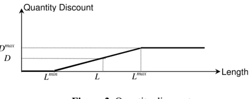
We observe two types of economies of scale: quantity discount, which applies to the variable component of pipe cost and contiguity discount, which applies to the mobilisation (fixed) component.

Figure 2 illustrates the concept for quantity discount: for a certain pipe material installed at a given year, unit cost discount is zero for a small quantity of pipes. When total quantity exceeds Lmin, quantity discount starts kicking in and increases with pipe length to a maximum of Dmax, which is obtained at quantities matching or exceeding Lmax.

Figure 2. Quantity discount

Contiguity discount is defined as follows: if pipe j is contiguous to pipe i (both share the same node) and both are replaced in a given year t they are assumed to be part of the same replacement project and therefore only one mobilization component is levied. Therefore, if k contiguous pipes are replaced in a given year, their total replacement cost will comprise the sum of all their unit costs plus one mobilization charge (i.e., k-1

Lmin Length Quantity Discount Lmax Dmax D L

mobilisation charges were saved compared to the cost of replacing k non-contiguous pipes).

In addition, we also consider the benefit of possible coordination of pipe replacement with scheduled roadwork. It is assumed that the unit cost (variable component) of pipe replacement is discounted by pi (e.g., $/m or % of cost) if pipe i is replaced at the same

year t that the pavement overlying it is scheduled for renewal. Equation (2) can now be modified to include all the savings described above:

rt t i t i t i t j soc i indir i rj wat i dir i rep i j i rt t i tot t i

e

savings

on

coordinati

Roadwork

discount

Quantity

savings

on

Mobilisati

C

C

e

C

C

C

k

e

CR

C

+

+

+

−

+

+

+

+

+

=

∑

)

(

]

)

[(

The total pipe replacement budget for the entire planning horizon of T years is denoted by B. We consider two budget scenarios, namely annual budget and non-restricted global budget. In the annual budget scenario, B is divided into annual portions Bt and

the total investment in pipe replacement in year t must not exceed Bt. The annual

portions Bt can be equal portions, increasing/decreasing series or arbitrary. In the

non-restricted scenario, B can be allocated to the planning period in the most economically efficient manner, where the only restriction is that the total pipe replacement costs in all years T cannot exceed B.

It is very important to note that for budgetary calculations pipe replacement costs (investments) are taken at their nominal values (including savings on economies of scale and timely coordination with scheduled roadwork renewal/replacement) and not at their present values.

5. Optimisation of replacement scheduling of pipes

The optimisation process has three major steps:

Step 1: Use I-WARP to produce a forecast of expected number of breaks for each pipe i in a homogeneous group of P pipes for each year t in the period of 2T+1 years, where T is the planning period.

Step 2: For each pipe i in P compute (equation 2) for each t in period 2T+1. Pipes for which t* (i.e., is minimum) occurs at year t = 2T+1 are not considered for replacement in planning period T and are removed from the analysis pipe set. The subset of the remaining pipes for analysis is denoted by P’.

tot t i C, tot t i C_,

Step 3: Use multi-objective genetic algorithm (MOGA) to find a set of non-inferior feasible solutions, or policies (Pareto front). GANetXL (Bicik, 2008), a

prototype non-commercial program (uses MS-Excel® as a platform) developed by the Centre for Water Systems (CWS) at the University of Exeter, UK was used in this study.

• The objectives for the MOGA are minimisation of total PV of costs (equation 2) and the maximisation of budget usage (minimisation of difference between available budget(s) and actual investment in pipe replacement). Note that budget and investment are considered at cash value while minimisation is done on the present value of costs.

• Imposition of budget constraint is achieved by penalising budget exceedance. • Quantity discounts and contiguity discounts have to be recalculated for each

candidate solution (policy).

• A policy may comprise pipes scheduled for replacement in year t ≤ T as well as pipes scheduled for replacement at year t > T. Within this policy only the former pipes are to be replaced within the planning period T. The latter are considered as pipes whose replacement is postponed to the next planning period.

6. Case study

We used a data set obtained from a water utility in Eastern Ontario, Canada. The utility has documented breakage records since 1972. The utility embarked on a hotspot cathodic protection program in 1984. For the analysis, 2 homogeneous groups of pipes were extracted. Group 1 comprised 6” (150 mm) diameter unlined cast iron (UCI) pipes installed in the 15-year period 1946-60, in total 391 individual pipe records (we

respected the utility’s definition of ‘individual pipe’ as was reflected in the database) with total length of about 54 km. Group 2 comprised 99 individual records of 8” (200 mm) diameter pipes of the same material and vintage, with total length of about 12 km. Pipes in both groups together formed a contiguous network (Figure 3). Climate data for the analysis years were obtained from Environment Canada.

6.1 Model training

I-WARP was applied to breaks recorded between 1972-2006 (training period). An examination of the coefficients (Table 1) reveals that background ageing is drastically different between the two groups. The length covariate in this case study was taken as the loge of pipe length. This means that in Group 1 the influencing factor is pipe length

to the power of approximately 2/3, while in Group 2 the power is greater than unity. The positive sign of PKNOF in Group 1 may point to a “worse than old” condition (in repairable systems three repair-related conditions are observed, “good as new”, “good as old” and “worse than old”). However, in Group 2, PKNOF was statistically

insignificant (at 5% significance level, using likelihood ratio test). The impact of

climate covariates on the model was statistically insignificant in Group 2 and somewhat inconsistent in Group 1, where freezing index (FI) showed little impact, snapshot rain deficit (RDs) appeared to have a more pronounced impact, and cumulative rain deficit (RDc) showed a relative larger impact but in a counter intuitive direction (negative coefficient). Water mains at this water utility are typically buried at a depth of 2.4 m, which may explain the low impact of FI, but not the negative sign of RDc. The positive coefficient of HSCP in Group 1 is also contrary to expectation, as it reflects that hotspot anodes act to increase (instead of reduce) breakage intensity.

Table 1. Coefficients obtained from model training using I-WARP

Group constant Ageing FI RDc RDs Length PKNOF HSCP

Group 1 -8.47 0.48 0.07 -0.41 0.34 0.65 0.76 0.43 Group 2 -11.97 0.74 N/S* N/S* N/S* 1.14 N/S* N/S* *Statistically not significant at 5% level, using likelihood ratio test.

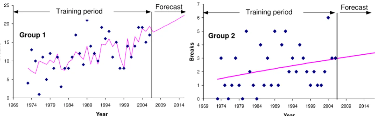
Figure 3 illustrates observed, and modeled number of breaks (aggregated by year) in the training period as well as the forecasted number of breaks for the two groups. Note that in Group 2, the modeled number of breaks is a rather smooth line because all time-dependent covariates were statistically insignificant and therefore removed from the analysis.

Figure 3. Network formed by 490 pipes in Groups 1 and 2

Figure 4. Trained models and forecasted breaks aggregated by year.

0 5 10 15 20 25 1969 1974 1979 1984 1989 1994 1999 2004 2009 2014 Year B rea ks 0 1 2 3 4 5 6 1969 1974 1979 1984 1989 1994 1999 2004 2009 2014 Year B re aks 7 Training period Group 1 Forecast Training period Group 2 Forecast

6.2 Pipe renewal planning

Corresponding to Step 1 (Section 5), planning period was selected as T = 5 years. Consequently, as can be seen in Figure 4, break forecast (using the coefficients from Table 1) was done for the 11 years 2007-2017 (forecast period that corresponds to 2T + 1). Although Figure 4 illustrates only the aggregated number of forecasted breaks, I-WARP provides a break forecast for each individual pipe.

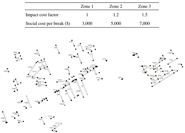
Corresponding to Step 2 (Section 5), we computed cost for each pipe i in period 2T+1. The unit costs used are provided in Tables 2 and 3. Zones in Table 3 represent different impact of pipe failure. Zone 1 represents low impact, e.g., industrial area; Zone 2 represents medium impact, e.g., residential area; and Zone 3 represents high impact, e.g., downtown area. Accordingly, each area is assigned different social cost of failure (Table 2) as well as an impact cost factor, used to multiply unit costs provided in Table 2. We consider a discount rate of r = 2%, which is in line with typical social discount rates (as opposed to financial discount rates) appropriate for public projects.

tot t i

C,

Pipes for which t* (i.e., C is minimum) occurs at year t = 2T+1 were not considered for replacement in planning period T and were therefore removed from the analysis pipe set. The subset of the remaining pipes comprised 105 (out of 490) individual mains. Their layout is illustrated in Figure 5.

tot t i,

We did not have real data on planned roadworks, instead we simulated roadwork schedule as follows. We assumed that the road above each of the 105 pipes would be renovated once in the 10 year period 2007-2016, in more or less equal portions each year. The year at which roadwork would be implemented was assigned by a random process using uniform distribution. Consequently, 57 (of 105) pipes saw planned roadwork during the 5-year planning period (Figure 5).

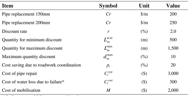
Table 2. Cost data

Item Symbol Unit Value

Pipe replacement 150mm Cr $/m 200

Pipe replacement 200mm Cr $/m 250

Discount rate r (%) 2.0

Quantity for minimum discount Lm in_m (m) 500 Quantity for maximum discount Lmax_m (m) 1,500 Maximum quantity discount d_mmax (%) 10 Cost saving due to roadwork coordination pi (%) 20

Cost of pipe repair Cirep ($) 3,000

Cost of water loss due to failure* Ciwat ($) 300

Cost of mobilisation M ($) 2,000

Table 3. Factors for cost assessment

Zone 1 Zone 2 Zone 3 Impact cost factor 1 1.2 1.5 Social cost per break ($) 3,000 5,000 7,000

Figure 5. 105 candidate pipes for renewal (grey background = planned roadwork)

In order to demonstrate the efficiency of the optimization process, we first examined a renewal policy, whereby only pipes whose is minimum for t = 1, 2, …5 are replaced (with no budget limitation). Table 4 provides a detailed summary of the outcome of this policy, to which we shall refer as the “baseline policy”.

tot t i

C_,

Next we applied the optimization process with a budget constrained that is

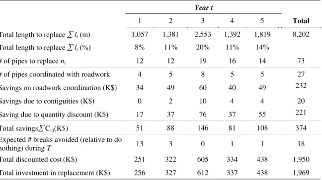
approximately equal to the total investment obtained in the baseline policy. Table 5 provides a detailed summary of outcome of this optimized policy. It is quite clear that the optimized policy is superior to the baseline policy, because while investing almost the same sum of money in replacement it allows for the replacement of an additional 772 m (more than 10% additional pipe length) of pipe and is expected to avoid one additional break compared to the baseline policy. It also provides a more balanced cash outlay compared to the baseline policy in which about half of the investment capital is expended in the first year.

Note that the total discounted cost in the optimized policy is higher than that in the baseline policy by about $24K. This is because the optimized policy encompasses 772m more replaced pipes compared to the baseline policy. One could therefore say that the optimal policy enabled the replacement of additional 772 meters of pipe at a marginal cost of about $31/m.

Table 4. Details of the baseline policy ($ values rounded to 1000)

Year t

1 2 3 4 5 Total

Total length to replace ∑ li (m) 3,838 1,222 151 1,134 1,085 7,430

Total length to replace ∑ li (%) _{30% 10% 1% 9% 8% 30%}

# of pipes to replace nt _{40 8 3 9 5 65}

# of pipes coordinated with roadwork _{10 1 0 1 1 13} Savings on roadwork coordination (K$) _{38 12 0 1 10 60} Savings due to contiguities (K$) _{16 2 0 0 0 18} Saving due to quantity discount (K$) _{115 26 0 22 19 182} Total savings∑ Ci,t(K$) 168 40 22 29 259 Expected # breaks avoided (relative to do

nothing) during 13 3 0 1 0 17

Total discounted cost (K$) _{959 320 44 312 290 1,926} Total investment in replacement (K$) _{979 326 45 32 297 1,965}

Table 5. Details of the optimised renewal policy ($ values rounded to 1000)

Year t

1 2 3 4 5 Total

Total length to replace ∑ li (m) 1,057 1,381 2,553 1,392 1,819 8,202

Total length to replace ∑ li (%) 8% 11% 20% 11% 14%

# of pipes to replace nt 12 12 19 16 14 73

# of pipes coordinated with roadwork 4 5 8 5 5 27 Savings on roadwork coordination (K$) 34 49 60 40 49 232 Savings due to contiguities (K$) 0 2 10 4 4 20 Saving due to quantity discount (K$) 17 37 76 37 55 221 Total savings∑ Ci,t(K$) 51 88 146 81 108 374 Expected # breaks avoided (relative to do

nothing) during T 13 3 0 1 1 18

Total discounted cost(K$) 251 322 605 334 438 1,950 Total investment in replacement (K$) 256 327 612 337 438 1,969

7. Summary and conclusions

A non-homogeneous Poisson process based model (I-WARP) is described, which considers three classes of covariates, pipe-dependent, time-dependent and pipe and time dependent. This model is used to forecast future water main breaks in each individual pipe. The forecasted numbers of break are then used for the efficient planning of water

main renewal in a short to medium planning period. The planning takes account of life cycle costs associated with the pipes and considers aspects of economies of scale, including quantity discount, contiguity savings due to reduced mobilization costs and coordination with anticipated road works (hence the need for short to medium planning period). Renewal planning can be done with or without budget constraint, where budget constraint can be global (for the entire planning period) or annual. This non-linear scheduling problem is discretized and solved using multi-objective genetic algorithm (MOGA). A case study, comprising a network of about 500 individual pipes was used to demonstrate the modeling and the planning process.

The approach for planning the replacement of individual water mains, is currently limited to the consideration of structural resiliency (i.e., breakage frequency) of pipes and the economics of their replacement. In reality, other factors should also be considered as well, such as hydraulic, reliability, etc. More work is required to incorporate additional considerations into this approach.

Acknowledgement

The pipe deterioration modeling part in this paper is based on a research project co-funded by the Water Research Foundation (formerly known as the American Water Works Association Research Foundation – AwwaRF) and the NRC and supported by water utilities from the United States and Canada.

References

Andreou, S. A., Marks, D. H., and Clark, R. M. (1987). “A new methodology for modeling break failure patterns in deteriorating water distribution systems: Theory.” Advance in Water Resources, 10, 2-10. Bicik, J., Morley, M.S., Savic, D.A. (2008). “A Rapid Optimization Prototyping Tool For

Spreadsheet-Based Models”, Proceedings of the 10th Annual Water Distribution Systems Analysis Conference (WDSA2008), Kruger National Park, South Africa, pp 472-482.

Boxall, J. B., A. O’Hagen, S. Pooladsaz, A. Saul, and D. Unwin, (2007). Estimation of burst rate in water distribution mains”, Proceedings of the Institution of Civil Engineers, Water Management I60, Issue

WM2, pp 73-82. June.

Constantine, A. G., and Darroch, J. N. (1993). “Pipeline reliability: stochastic models in engineering technology and management.” S. Osaki, D.N.P. Murthy, eds., World Scientific Publishing Co. Dridi, L,. Mailhot, A., Parizeau, M., and Villeneuve J.P. (2005) “A strategy for optimal replacement of

water pipes integrating structural and hydraulic indicators based on a statistical water pipe break model”. Proceedings of the 8th International Conference on Computing and Control for the Water

Industry, U. of Exeter, UK, September, 65-70.

Giustolisi, O., Laucelli, D, and Savic D. A., (2005). “A decision support framework fro short time planning of rehabilitation”, Proceedings of Computer and Control in Water Indu stry (CCWI), (1), 39-44. Jarrett, R. O. Hussain, and J. Van der Touw (2003). “Reliability assessment of water pipelines using

limited data”, OzWater, Perth, Australia.

Kleiner, Y. and Rajani, B. (2001). “Comprehensive review of structural deterioration of water mains: statistical models”. Urban Water, (3), 131-150.

Kleiner, Y. and Rajani, B. (2004). “Quantifying effectiveness of cathodic protection in water mains: theory,” Journal of Infrastructure Systems, ASCE, 10,(2), 43-51.

Kleiner, Y., and B. Rajani, (2008). “Prioritising individual water mains for renewal," ASCE/EWRI World

Environmental and Water Resources Congress (Honolulu, Hawaii, May 12.

Le Gat, Y. (2007). “Extending the Yule Process to model recurrent failures of pressure pipes”,Private communication.

Mailhot, A., A. Paulin, and Villeneuve J-P, (2003). “Optimal replacement of water pipes”, Water

Nafi, A. and Y. Kleiner, (2009). “Scheduling of water pipes renewal by considering adjacency of infrastructure works and economy of scale” in preparation.

Røstum, J. (2000). “Statistical modelling of pipe failures in water networks”. PhD thesis, Norwegian University of Science and Technology, Trondheim, Norway.

Park, S. and G. V. Loganathan (2002). “Optimal pipe replacement analysis with a new pipe break prediction model” Journal of the Korean Society of Water and Wastewater, 16/6, pp. 710-716. Watson, T.G., C.D. Christian, A. J., Mason, M. H. Smith, and R. Meyer (2004). “Bayesian-based pipe