Bayesian nonparametric reward learning from demonstration

Bayesian Nonparametric Reward Learning

from Demonstration

by

AASACHUS ETTS iNS E

Bernard J. Michini

"EAE

S.M., Aeronautical/Astronautical Engineering

~

Massachusetts Institute of Technology (2009)

NOV 2

2013

S.B., Aeronautical/Astronautical Engineering

Massachusetts Institute of Technology (2007)

Submitted to the Department of Aeronautics and Astronautics

in partial fulfillment of the requirements for the degree of

Doctor of Philosophy in Aeronautics and Astronautics

at the

MASSACHUSETTS INSTITUTE OF TECHNOLOGY

August 2013

@

Massachusetts Institute of Technology 2013. All rights reserved.

A uth or ....

...

Department of

C ertified by ...

Richard C. Maclaurin Professor of

. A

Certified by..

Associate Professor of

Certified by..

A4socifte Professor of

Aeronautics and Astronautics

August, 2013

...

Jonathan P. How

Aeronautics and Astronautics

Thesis Supervisor

...

Nicholas Roy

Aeronautics and Astronautics

...

...

Mary Cummings

Aeronautics and Astronautics

Accepted by ...

...

Eytan H. Modiano

Professor of Aeronautics and Astronautics

Chair, Graduate Program Committee

(VI

Bayesian Nonparametric Reward Learning

from Demonstration

by

Bernard J. Michini

Submitted to the Department of Aeronautics and Astronautics on August, 2013, in partial fulfillment of the

requirements for the degree of

Doctor of Philosophy in Aeronautics and Astronautics

Abstract

Learning from demonstration provides an attractive solution to the problem of teach-ing autonomous systems how to perform complex tasks. Demonstration opens au-tonomy development to non-experts and is an intuitive means of communication for humans, who naturally use demonstration to teach others. This thesis focuses on a specific form of learning from demonstration, namely inverse reinforcement learning, whereby the reward of the demonstrator is inferred. Formally, inverse reinforcement learning (IRL) is the task of learning the reward function of a Markov Decision Process (MDP) given knowledge of the transition function and a set of observed demonstra-tions. While reward learning is a promising method of inferring a rich and trans-ferable representation of the demonstrator's intents, current algorithms suffer from intractability and inefficiency in large, real-world domains. This thesis presents a reward learning framework that infers multiple reward functions from a single, unseg-mented demonstration, provides several key approximations which enable scalability to large real-world domains, and generalizes to fully continuous demonstration do-mains without the need for discretization of the state space, all of which are not handled by previous methods.

In the thesis, modifications are proposed to an existing Bayesian IRL algorithm to improve its efficiency and tractability in situations where the state space is large and the demonstrations span only a small portion of it. A modified algorithm is presented and simulation results show substantially faster convergence while main-taining the solution quality of the original method. Even with the proposed efficiency improvements, a key limitation of Bayesian IRL (and most current IRL methods) is the assumption that the demonstrator is maximizing a single reward function. This presents problems when dealing with unsegmented demonstrations containing mul-tiple distinct tasks, common in robot learning from demonstration (e.g. in large tasks that may require multiple subtasks to complete). A key contribution of this thesis is the development of a method that learns multiple reward functions from a single demonstration. The proposed method, termed Bayesian nonparametric in-verse reinforcement learning (BNIRL), uses a Bayesian nonparametric mixture model

to automatically partition the data and find a set of simple reward functions corre-sponding to each partition. The simple rewards are interpreted intuitively as subgoals, which can be used to predict actions or analyze which states are important to the demonstrator. Simulation results demonstrate the ability of BNIRL to handle cyclic tasks that break existing algorithms due to the existence of multiple subgoal rewards in the demonstration. The BNIRL algorithm is easily parallelized, and several ap-proximations to the demonstrator likelihood function are offered to further improve computational tractability in large domains.

Since BNIRL is only applicable to discrete domains, the Bayesian nonparametric reward learning framework is extended to general continuous demonstration domains

using Gaussian process reward representations. The resulting algorithm, termed

Gaussian process subgoal reward learning (GPSRL), is the only learning from demon-stration method that is able to learn multiple reward functions from unsegmented demonstration in general continuous domains. GPSRL does not require discretiza-tion of the continuous state space and focuses computadiscretiza-tion efficiently around the demonstration itself. Learned subgoal rewards are cast as Markov decision process options to enable execution of the learned behaviors by the robotic system and provide a principled basis for future learning and skill refinement. Experiments conducted in the MIT RAVEN indoor test facility demonstrate the ability of both BNIRL and GP-SRL to learn challenging maneuvers from demonstration on a quadrotor helicopter and a remote-controlled car.

Thesis Supervisor: Jonathan P. How

Acknowledgments

Foremost, I'd like to thank my family and friends. None of my accomplishments would be possible without their constant support. To Mom, Dad, Gipper, Melissa, and the rest of my family: there seems to be very little in life that can be counted on, yet you have proven time and again that no matter what happens you will always be there for me. It has made more of a difference than you know. To the many many wonderful friends I've met over the last 10 years at the Institute (of whom there are too many to name), and to the men of Phi Kappa Theta fraternity who I've come to consider my brothers: despite the psets, projects, and deadlines, you've made life at MIT the most enjoyable existence I could ask for. I constantly think on the time we shared, both fondly and jealously, and I truly hope that we continue to be a part of each others lives.

I'd also like to thank the academic colleagues who have given me so much assis-tance during my time as a graduate student. To my advisor, Professor Jon How: it's been my pleasure to learn your unique brand of research, problem solving, technical writing, and public speaking, and I'm extremely grateful for your mentorship over the years (though I sometimes hear "what's the status" in my sleep). Thanks also to my thesis committee, Professors Missy Cummings and Nicholas Roy, for their guidance and support. To the many past and present members of the Aerospace Controls Lab, including Dan Levine, Mark Cutler, Luke Johnson, Sam Ponda, Josh Redding, Frant Sobolic, Brett Bethke, and Brandon Luders: I couldn't have asked for a better group of colleagues to spend the many work days and late nights with. I wish you all the best of luck in your professional careers.

Finally, I'd like to thank the Office of Naval Research Science of Autonomy pro-gram for funding this work under contract #N000140910625.

Contents

1 Introduction

1.1 Motivation: Learning from Demonstration in Autonomy

1.2 Problem Formulation and Solution Approach . . . .

1.3 Literature Review 1.4 1.5 Summary of Contributions . . . . Thesis Outline. . . . . 2 Background

2.1 Markov Decision Processes and Options .

2.2 Inverse Reinforcement Learning . . . . .

2.3 Chinese Restaurant Process Mixtures . .

2.4 CRP Inference via Gibbs Sampling . . .

2.5 Gaussian Processes . . . .

2.6 Sum m ary . . . .

3 Improving the Efficiency of Bayesian IRL

3.1 Bayesian IRL . . . .

3.2 Limitations of Standard Bayesian IRL

3.2.1 Room World MDP . . . .

3.2.2 Applying Bayesian IRL . . . .

3.3 Modifications to the BIRL Algorithm . .

3.3.1 Kernel-based Relevance Function

3.3.2 Cooling Schedule . . . . 17 18 19 . . . . 2 1 24 28 31 . . . . 31 . . . . 33 . . . . 34 . . . . 36 . . . . 40 . . . . 42 45 47 50 50 51 53 53 54

3.4 Simulation Results . . . .

3.5 Sum m ary . . . .

4 Bayesian Nonparametric Inverse Reinforcement Learning

4.1 Subgoal Reward and Likelihood Functions . . . . . 4.2 Generative Model . . . . 4.3 Inference . . . . 4.4 Convergence in Expected 0-1 Loss . . . . 4.5 Action Prediction . . . . 4.6 Extension to General Linear Reward Functions . . . 4.7 Simulation Results . . . . 4.7.1 Grid World Example . . . . 4.7.2 Grid World with Features Comparison . . . 4.7.3 Grid World with Loop Comparison . . . . . 4.7.4 Comparison of Computational Complexities 4.8 Sum m ary . . . .

5 Approximations to the Demonstrator Likelihood

5.1 Action Likelihood Approximation . . . .

5.1.1 Real-time Dynamic Programming . . . .

5.1.2 Action Comparison . . . .

5.2 Simulation Results . . . .

5.2.1 Grid World using RTDP . . . .

5.2.2 Pedestrian Subgoal Learning using Action Comparison .

5.3 Sum m ary . . . .

6 Gaussian Process Subgoal Reward Learning

6.1 Gaussian Process Subgoal Reward Learning Algorithm . . . . .

6.2 Subgoal Reward Representation . . . .

6.3 Action Likelihood . . . .

6.4 Gaussian Process Dynamic Programming . . . .

55 58 61 . . . . 62 . . . . 63 . . . . 65 . . . . 68 . . . . 70 . . . . 70 . . . . 71 . . . . 72 . . . . 72 . . . . 74 . . . . 76 . . . . 80 83 84 85 87 89 89 90 92 95 95 96 98 98

6.5 Bayesian Nonparametric Mixture Model and Subgoal Posterior Inference 99

6.6 Converting Learned Subgoals to MDP Options . . . . 100

6.7 Sum m ary . . . . 101

7 Experimental Results 103 7.1 Experimental Test Facility . . . . 103

7.2 Learning Quadrotor Flight Maneuvers from Hand-Held Demonstration with Action Comparison . . . . 104

7.3 Learning Driving Maneuvers from Demonstration with GPSRL . . . . 105

7.3.1 Confidence Parameter Selection and Expertise Determination 108 7.3.2 Autonomous Execution of Learned Subgoals . . . . 110

8 Conclusions and Future Work 117 8.1 Future W ork . . . . 120

8.1.1 Improved Posterior Inference . . . . 120

8.1.2 Sparsification of Demonstration Trajectories . . . . 121

8.1.3 Hierarchical Reward Representations . . . . 121

8.1.4 Identifying Multiple Demonstrators . . . . 122

List of Figures

2-1 Example of Gibbs sampling applied to CRP mixture model . . . . 39

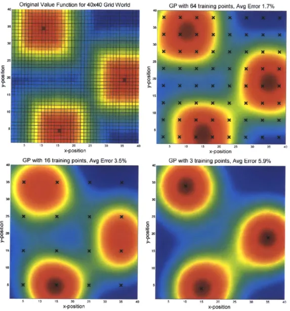
2-2 Example of Gaussian process approximation of Grid World value function 43

3-1 Room World MDP with example expert demonstration. . . . . 50

3-2 Reward function prior distribution (scaled). . . . . 52

3-3 State relevance kernel scores for narrow and wide state relevance kernels. 57

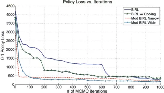
3-4 Comparison of 0-1 policy losses vs. number of MCMC iterations. . . . 58

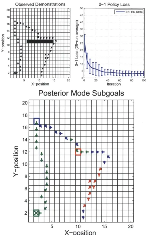
4-1 Observed state-action pairs for simple grid world example, 0-1 policy

loss for Bayesian nonparametric IRL, and posterior mode of subgoals

and partition assignments. . . . . 73

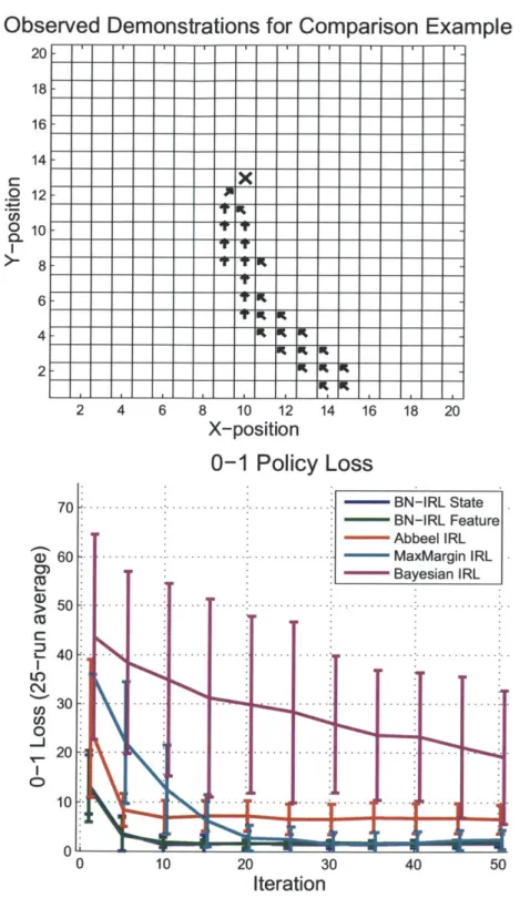
4-2 Observed state-action pairs for grid world comparison example and

comparison of 0-1 Policy loss for various IRL algorithms. . . . . 75

4-3 Observed state-action pairs for grid world loop example, comparison

of 0-1 policy loss for various IRL algorithms, and posterior mode of

subgoals and partition assignments . . . . 77

5-1 Progression of real-time dynamic programming sample states for the

Grid W orld example . . . . 86

5-2 Two-dimensional quadrotor model, showing y, z, and 6 pose states

along with i, %, and 6 velocity states. . . . . 88

5-3 Comparison of average CPU runtimes for various IRL algorithms for

the Grid World example, and the average corresponding 0-1 policy loss

5-4 Simulation results for pedestrian subgoal learning using action com-parison. Number of learned subgoals versus sampling iteration for a

representative trial . . . . 93

7-1 RAVEN indoor test facility with quadrotor flight vehicles, ground

ve-hicles, autonomous battery swap and recharge station, and motion

capture system . . . . 104

7-2 A human demonstrator motions with a disabled quadrotor. The BNIRL

algorithm with action comparison likelihood converges to a mode pos-terior with four subgoals. An autonomous quadrotor takes the subgoals as waypoints and executes the learned trajectory in actual flight . . . 106

7-3 A cluttered trajectory and the BNIRL posterior mode. The BNIRL

posterior mode is shown in red, which consists of four subgoals, one at

each corner of the square as expected . . . . . 107

7-4 A hand-held demonstrated quadrotor flip, the BNIRL posterior mode, and an autonomous quadrotor executing the learned trajectory in

ac-tual flight . . . . 111

7-5 RC car used for experimental results and diagram of the car state

variables . . . . 111

7-6 Thirty-second manually-controlled demonstration trajectory and the

six learned subgoal state locations . . . . 112

7-7 Number of subgoals learned versus the total length of demonstration

data sampled, averaged over 25 trials . . . . 113

7-8 Demonstration with three distinct right-turning radii, and number of

learned subgoals (50-trial average) versus the confidence parameter valu e ce . . . . 114

7-9 Comparison of demonstrated maneuvers to the autonomous execution

List of Algorithms

1 Generic inverse reinforcement learning algorithm . . . . 35

2 Generic CRP mixture Gibbs sampler . . . . 38

3 Modified BIRL Algorithm . . . . 55

4 Bayesian nonparametric IRL . . . . 67

List of Tables

Chapter 1

Introduction

As humans, we perform a wide variety of tasks every day: determining when to leave home to get to work on time, choosing appropriate clothing given a typically-inaccurate weather forecast, braking for a stoplight with adequate margin for error (and other drivers), deciding how much cash to withdraw for the week's expenses, tak-ing an exam, or locattak-ing someone's office in the Stata Center. While these tasks may seem mundane, most are deceivingly-complex and involve a myriad of pre-requisites like motor skills, sensory perception, language processing, social reasoning, and the ability to make decisions in the face of uncertainty.

Yet we are born with only a tiny fraction of these skills, and a key method of filling the gap is our incredible ability to learn from others. So critical is the act of learning that we spend our entire lifetime doing it. While we often take for granted its complexities and nuances, it is certain that our survival and success in the world are directly linked to our ability to learn.

A direct analogy can be drawn to robotic (and more generally autonomous)

sys-tems. As these systems grow in both complexity and role, it seems unrealistic that they will be programmed a priori with all of the skills and behaviors necessary to perform complex tasks. An autonomous system with the ability to learn from others has the potential to achieve far beyond its original design. While the notion of a robot with a human capacity for learning has long been a coveted goal of the artificial intelligence community, a multitude of technical hurdles have made realization of such

of a goal extremely difficult. Still, much progress has been and continues to be made using the tools available, highlighting the potential for an exciting future of capable autonomy.

1.1

Motivation: Learning from Demonstration in

Autonomy

As technology continues to play a larger role in society, humans interact with au-tonomous systems on a daily basis. Accordingly, the study of human-robot interac-tion has seen rapid growth [29, 34, 39, 47, 64, 85, 92]. It is reasonable to assume that non-experts will increasingly interact with robotic systems and will have an idea of how the system should act. For the most part, however, autonomy algorithms are currently developed and implemented by technical experts such as roboticists and computer programmers. Modifying the behavior of these algorithms is mostly beyond the capabilities of the end-user. Learning from demonstration provides an attractive solution to this problem for several reasons [6]. The demonstrator is typically not required to have expert knowledge of the domain dynamics. This opens autonomy development to non-robotics-experts and also reduces performance brittleness from model simplifications. Also, demonstration is already an intuitive means of communi-cation for humans, as we use demonstration to teach others in everyday life. Finally, demonstrations can be used to focus the automated learning process on useful areas of the state space [53], as well as provably expand the class of learnable functions

[97].

There have been a wide variety of successful applications that highlight the utility and potential of learning from demonstration. Many of these applications focus on teaching basic motor skills to robotic systems, such as object grasping [83, 89, 96], walking [58], and quadraped locomotion [48, 73]. More advanced motor tasks have also been learned, such as pole balancing [7], robotic arm assembly [19], drumming [43], and egg flipping [67]. Demonstration has proved successful in teaching robotic

systems to engage in recreational activities such as soccer [4, 40, 41], air hockey [11], rock-paper-scissors [18], basketball [17], and even music creation [32]. While the pre-vious examples are focused mainly on robotics, there are several instances of learning from demonstration in more complex, high-level tasks. These include autonomous driving [2, 21, 66], obstacle avoidance and navigation [44, 82], and unmanned

acro-batic helicopter flight [23, 63].

1.2

Problem Formulation and Solution Approach

This thesis focuses on learning from demonstration, a demonstration being defined as a set of state-action pairs:

0

where 0 is the demonstration set, si is the state of the system, and a is the action that was taken from state si. In the thesis, it is assumed that states and actions are fully-observable, and problems associated with partial state/action observability are not considered. The demonstration may not necessarily be given in temporal order, and furthermore could contain redundant states, inconsistent actions, and noise resulting from imperfect measurements of physical robotic systems.

Learning from demonstration methods can be distinguished by what is learned from the demonstration. Broadly, there are two classes: those which attempt to learn

a policy from the demonstration, and those which attempt to learn a task

descrip-tion from the demonstradescrip-tion. In policy learning methods, the objective is to learn

a mapping from states to actions that is consistent with the state-action pairs ob-served in the demonstration. In that way, the learned policy can be executed on the autonomous system to generate behavior similar to that of the demonstrator.

Policy methods are not concerned with what is being done in the demonstration, but rather how it is being done. In contrast, task learning methods use the demonstra-tion to infer the objective that the demonstrator is trying to achieve. A common way

of specifying such an objective is to define an associated reward function, a mapping from states to a scalar reward value. The task can then be more concretely defined as reaching states that maximize accumulated reward. This thesis focuses primarily on the problem of reward learning from demonstration.

Reward learning is challenging for several fundamental reasons:

" Learning rewards from demonstration necessitates a model of the demonstra-tor that predicts what actions would be taken given some reward function (or objective). The actions predicted by the model are compared to the demon-stration as a means of inferring the reward function of the demonstrator. The demonstrator model is typically difficult to obtain in that it requires solving for a policy which maximizes a candidate reward function.

" The demonstration typically admits many possible corresponding reward func-tions, i.e. there is no unique reward function that explains a given set of observed state-action pairs.

" The demonstration itself can be inconsistent and the demonstrator imperfect. Thus, it cannot be assumed that the state-action pairs in the demonstration optimize reward, only that they attempt to do so.

Despite these difficulties, reward learning has several perceived advantages over policy learning. A policy, due to its nature as a direct mapping from states to actions, becomes invalid if the state transition model changes (actions may have different consequences than they did in the original demonstration). Also, a policy mapping must be defined for every necessary state, relying on a large demonstration set or additional generalization methods. A learned reward function, however, can be used to solve for a policy given knowledge of the state transition model, making it invariant to changes in domain dynamics and generalizable to new states. Thus, a reward function is a succinct and transferable description of the task being demonstrated and still provides a policy which generates behavior similar to that of the demonstrator.

This thesis focuses primarily on developing reward learning from demonstration techniques that are scalable to large, real-world, continuous demonstration domains

while retaining computational tractability. While previous reward learning methods assume that a single reward function is responsible for the demosntration, the frame-work developed in this thesis is based on the notion that the demonstration itself can be partitioned and explained using a class of simple reward functions. Two new reward learning methods are presented that utilize Bayesian nonparametric mixture models to simultaneously partition the demonstration and learn associated reward functions. Several key approximation methods are also developed with the aim of improving efficiency and tractability in large continuous domains. Simulation results are given which highlight key properties and advantages, and experimental results validate the new algorithms applied to challenging robotic systems.

The next section highlights relevant previous work in the field of learning from demonstration, and is followed by a more detailed summary of the thesis contribu-tions.

1.3

Literature Review

The many methods for learning from demonstration can be broadly categorized into two main groups based on what is being learned [6]: a policy mapping function from states to actions, or a task description.

In the policy mapping approach, a function is learned which maps states to actions in either a discrete (classification) or continuous (regression) manner. Classification architectures used to learn low-level tasks include Gaussian Mixture Models for car driving [20], decision trees for aircraft control [77], and Bayesian networks [44] and k-Nearest Neighbors [78] for navigation and obstacle avoidance. Several classifiers have also been used to learn high-level tasks including Hidden Markov Models for box sorting [76] and Support Vector Machines for ball sorting [21]. Continuous regression methods are typically used to learn low-level motion-related behaviors, and a few of the many examples include Neural Networks for learning to drive on various road types [66], Locally-Weighted Regression [22] for drumming and walking [43, 58], and Sparse Online Gaussian Processes for basic soccer skills [41]. Actions are often defined

along with a set of necessary pre-conditions and resulting post-conditions [33]. Some examples include learning object manipulation [50], ball collection [94], navigation

from natural language dialog [51], and single-demonstration learning [36].

Of the learning from demonstration methods which learn a task description, most do so by learning a reward function. In [7], the transition model is learned from repeated attempts to perform an inverted pendulum task, and the reward function (the task itself) is learned from human demonstrations. The demonstrations double as a starting point for the policy search to focus the computation on a smaller volume of the state space. Similar approaches approaches are taken in [28, 36, 93]. When the transition function is assumed to be known (at least approximately), a reward function can be found that rationalizes the observed demonstrations. In the context of control theory this problem is known as Inverse Optimal Control, originally posed by Kalman

and solved in [16]. Ng and Russell cast the problem in the reinforcement learning

framework in [62] and called it Inverse Reinforcement Learning (IRL), highlighting the fact that the reward function in many RL applications is often not known a priori and must instead be learned. IRL seeks to learn the reward function which is argued in [62] to be the "most succinct, robust, and transferable definition of the task".

There have since been a number of IRL methods developed, many of which use

a weighted-features representation for the unknown reward function. Abbeel and

Ng solve a quadratic program iteratively to find feature weights that attempt to match the expected feature counts of the resulting policy with those of the expert demonstrations [2]. A game-theoretic approach is taken in [90], whereby a minimax search is used to minimize the difference in weighted feature expectations between the demonstrations and learned policy. In this formulation, the correct signs of the feature weights are assumed to be known and thus the learned policy can perform better than the expert. Ratliff et al. [73, 74] take a max-margin approach, finding a weight vector that explains the expert demonstrations by essentially optimizing the margin between competing explanations. Ziebart et al. [99, 100] match feature counts using the principle of maximum entropy to resolve ambiguities in the resulting reward function. In [61], the parameters of a generic family of parametrized rewards

are found using a more direct gradient method which focuses on policy matching with the expert. Finally, Ramachandran and Amir [71] take a general Bayesian approach, termed Bayesian Inverse Reinforcement Learning (BIRL).

All of the aforementioned IRL algorithms are similar in that they attempt to find a single reward function that explains the entirety of the observed demonstration. This reward function must then be necessarily complex in order to explain the data suffi-ciently, especially when the task being demonstrated is itself complicated. Searching for a complex reward function is fundamentally difficult for two reasons. First, as the complexity of the reward model increases, so too does the number of free parameters needed to describe the model. Thus the search is over a larger space of candidate functions. Second, the process of testing candidate reward functions requires solving for the MDP value function, the computational cost of which typically scales poorly with the size of the MDP state space, even for approximate solutions [13]. Thus find-ing a sfind-ingle, complex reward function to explain the observed demonstrations requires searching over a large space of possible solutions and substantial computational effort to test each candidate.

The algorithms presented in this thesis avoid the search for a single reward func-tion by instead partifunc-tioning the demonstrafunc-tion and inferring a reward funcfunc-tion for each partition. This enables the discovery of multiple reward functions from a single, unsegmented demonstration. Several methods have been developed that also address the issue of multimodal learning from unsegmented demonstration. Grollman et al. characterize the demonstration as a mixture of Gaussian process experts [41] and find multiple policies to describe the demonstration. Also using a Bayesian nonparametric framework, Fox et al. cast the demonstration as a switched linear dynamic system, and infer a hidden Markov model to indicate switching between systems [35]. In Con-structing Skill Trees (CST) the overall task is represented as a hierarchy of subtasks, and Markov decision process options (skills) are learned for each subtask. [49]. Of these methods, none attempt to learn multiple reward functions from unsegmented demonstration.

explain partitioned demonstration data. The notion of defining tasks using a cor-responding subgoal was proposed by Sutton et al. along with the options MDP framework [88]. Many other methods exist which learn options from a given set of trajectories. In [55], diverse density across multiple solution paths is used to dis-cover such subgoals. Several algorithms use graph-theoretic measures to partition densely-connected regions of the state space and learn subgoals at bottleneck states [56, 81]. Bottleneck states are also identified using state frequencies [84] or using a local measure of relative novelty [80]. Of these methods, most require large amounts of trajectory data and furthermore none have the ability to learn reward functions from demonstration.

1.4

Summary of Contributions

This thesis focuses broadly on improving existing reward learning from demonstration methods and developing new methods that enable scalable reward learning for real-world robotic systems. A reward learning framework is developed that infers multiple reward functions from a single, unsegmented demonstration, provides several key approximations which enable scalability to large real-world domains, and generalizes to fully continuous demonstration domains without the need for discretization of the state space, none of which are handled by previous methods.

The first contribution of the thesis is the proposal of several modifications to the Bayesian IRL algorithm to improve its efficiency and tractability in situations where the state space is large and the demonstrations span only a small portion of it. The key insight is that the inference task should be focused on states that are similar to those encountered by the expert, as opposed to making the naive assumption that the expert demonstrations contain enough information to accurately infer the reward function over the entire state space. With regard to the improvement of Bayesian IRL, the thesis makes the following contributions:

* Two key limitations of the Bayesian IRL algorithm are identified. Foremost, it is shown that the set of demonstrations given to the algorithm often contains

a limited amount of information relative to the entire state space. Even so, standard BIRL will attempt to infer the reward of every state. Second, the MCMC sampling in BIRL must search over a reward function space whose dimension is the number of MDP states. Even for toy problems, the number of MCMC iterations needed to approximate the mean of the posterior will become intractably large.

" A fundamental improvement is proposed which introduces a kernel function quantifying similarity between states. The BIRL inference task is then scaled down to include only those states which are similar to the ones encountered by the expert (the degree of "similarity" being a parameter of the algorithm). The resulting algorithm is shown to have much improved computational efficiency while maintaining the quality of the resulting reward function estimate. If the kernel function provided is simply a constant, the original BIRL algorithm is obtained.

* A new acceptance probability is proposed similar to a cooling schedule in Sim-ulated Annealing to improve speed of convergence to the BIRL prior mode. Use of the cooling schedule in the modified BIRL algorithm allows the MCMC process to first find areas of high posterior probability and focus the samples towards them, speeding up convergence.

Even with the proposed efficiency improvements, a key limitation of Bayesian IRL (and most current IRL methods) is the assumption that the demonstrator is

maximizing a single reward function. This presents problems when dealing with

unsegmented demonstrations containing multiple distinct tasks, common in robot learning from demonstration (e.g. in large tasks that may require multiple subtasks to complete). The second contribution of this thesis is the development of a method that learns multiple reward functions from a single demonstration. With respect to learning multiple reward functions, the thesis makes the following contributions:

* A new reward learning framework is proposed, termed Bayesian nonparametric inverse reinforcement learning (BNIRL), which uses a Bayesian

nonparamet-ric mixture model to automatically partition the data and find a set of simple reward functions corresponding to each partition. The simple rewards are inter-preted intuitively as subgoals, which can be used to predict actions or analyze which states are important to the demonstrator.

* Convergence of the BNIRL algorithm in 0-1 loss is proven. Several compu-tational advantages of the method over existing IRL frameworks are shown, namely the search over a finite (as opposed to infinite) space of possible rewards and the ability to easily parallelize the majority of the method's computational requirements.

" Simulation results are given for simple examples showing comparable perfor-mance to other IRL algorithms in nominal situations. Moreover, the proposed method handles cyclic tasks (where the agent begins and ends in the same state) that would break existing algorithms without modification due to the existence

of multiple subgoal rewards in a single demonstration.

" Two approximations to the demonstrator likelihood function are developed to further improve computational tractability in large domains. In the first method, the Real-time Dynamic Programming (RTDP) framework is incorpo-rated to approximate the optimal action-value function. RTDP effectively limits computation of the value function only to necessary areas of the state space. This allows the complexity of the BNIRL reward learning method to scale with the size of the demonstration set, not the size of the full state space. Simula-tion results for a Grid World domain show order of magnitude speedups over exact solvers for large grid sizes. In the second method, an existing closed-loop controller takes the place of the optimal value function. This avoids having to specify a discretization of the state or action spaces, extending the applicability of BNIRL to continuous demonstration domains when a closed-loop controller is available. Simulation results are given for a pedestrian data set, demonstrating the ability to learn meaningful subgoals using a very simple closed-loop control law.

While BNIRL has the ability to learn multiple reward functions from a single demonstration, it is only generally applicable in discrete domains when a closed-loop controller is not available. A main focus area of the thesis is achieving scalable reward learning from demonstration in real-world robotic systems, necessitating the extension of the Bayesian nonparametric reward learning framework to general, continuous demonstration domains. With respect to reward learning in continuous domains, this thesis makes the following contributions:

" The Bayesian nonparametric reward learning framework is extended to general continuous demonstration domains using Gaussian process reward representa-tions. The resulting algorithm, termed Gaussian process subgoal reward learn-ing (GPSRL), is the only learnlearn-ing from demonstration method able to learn multiple reward functions from unsegmented demonstration in general contin-uous domains. GPSRL does not require discretization of the contincontin-uous state space and focuses computation efficiently around the demonstration itself. " Learned subgoal rewards are cast as Markov decision process options to enable

execution of the learned behaviors by the robotic system and provide a prin-cipled basis for future learning and skill refinement. Definitions of the option initiation set, terminating criteria, and policy follow directly from data already inferred during the GPSRL reward learning process. This enables execution of learned subgoals without the requirement for further learning.

" A method is developed for choosing the key confidence parameter in the GPSRL

likelihood function. The method works by instructing the demonstrator to

execute a single maneuver several times, and doing a sweep of the parameter to identify regions of under- and over-fitting. Furthermore, this method can be used to quantify the relative skill level of the demonstrator, enabling comparison between multiple demonstrators.

Since the broad focus of this work is to enable scalable reward learning from demonstration, the final contribution of the thesis is to provide experimental results

demonstrating the ability of the proposed methods to learn reward from demonstra-tions in real-world robotic domains. With respect to experimental validation of the methods presented herein, the thesis makes the following contributions:

" Quadrotor flight maneuvers are learned from a human demonstrator using only hand motions. The demonstration is recorded using a motion capture system and then analyzed by the BNIRL algorithm with action comparison. Learned subgoal rewards (in the form of waypoints) are passed as commands to an autonomous quadrotor which executes the learned behavior in actual flight. The entire process from demonstration to reward learning to robotic execution takes on the order of 10 seconds to complete using a single computer. Thus, the results highlight the ability of BNIRL to use data from a safe (and not necessarily dynamically feasible) demonstration environment and quickly learn subgoal rewards that can be used in the actual robotic system.

" GPSRL is experimentally applied to a robotic car domain. In the experiments, multiple difficult maneuvering skills such as drifting turns are identified from a single unsegmented demonstration. The learned subgoal rewards are then executed autonomously using MDP options and shown to closely match the original demonstration. Finally, the relative skill level of the demonstrator is quantified through a posteriori analysis of the confidence likelihood parameter.

1.5

Thesis Outline

The thesis proceeds as follows. Chapter 2 provides background material on the math-ematical concepts that the thesis builds on. Chapter 3 presents several fundamental modifications to the existing Bayesian IRL method to improve efficiency and tractabil-ity in large domains. In Chapter 4, a new Bayesian nonparametric reward learning framework is developed enabling the discovery of multiple reward functions from a sin-gle demonstration. Chapter 5 offers several approximations to the BNIR.L likelihood function that further enables scalability to large domains. In Chapter 6, the GPSRL

algorithm is developed as a generalized, continuous extension of BNIRL. Chapter 7 provides experimental results demonstrating the application of BNIRL and GPSRL to quadrotor helicopter and remote-controlled car domains. Finally, Chapter 8 offers concluding remarks and highlights areas for future research.

Chapter 2

Background

This chapter provides a background in the mathematical concepts that this thesis builds upon. Throughout the thesis, boldface is used to denote vectors and subscripts are used to denote the elements of vectors (i.e. zi is the ith element of vector z).

2.1

Markov Decision Processes and Options

A finite-state Markov Decision Process (MDP) [69] is a tuple (S, A, T, R, -Y) where

S is a set of states, A is a set of actions, T : S x A x S -+ [0,1] is the function of

transition probabilities such that T(s, a, s') is the probability of being in state s' after

taking action a from state s, R : S -4 R is the reward function, and - E [0, 1) is the

discount factor.

A stationary policy is a function Tr : S H- A. From [87] we have the following set

of definitions and results:

1. The infinite-horizon expected reward for starting in state s and following policy 7r thereafter is given by the value function V'(s, R):

V'(s, R) = E, E -YR(si) SO = s (2.1)

i=O

where si is the state at time i. Assuming state-based reward (i.e. rewards that do not depend on actions), the value function satisfies the following Bellman

equation for all s E S:

V'(s, R) = R(s) + -y T(s, -r (s), s')V'(s') (2.2)

The so-called Q-function (or action-value function) Q"(s, a, R) is defined as the infinite-horizon expected reward for starting in state s, taking action a, and

following policy 7r thereafter:

Q"(s, a, R) = R(s) + -y T(s, a, s')V'(s') (2.3)

2. A policy -r is optimal iff, for all s E S:

7r (s) = argmax

Q'(s,

aEA

An optimal policy is denoted as 7r* with corresponding value function V* and

action-value function Q*.

There are many methods available for computing or approximating V* (and thus

Q*)

Vk1(s, R) = R(s) + maxZy T(s, a, s')Vk (s') Vs

E S

a

The sequence {Vk} can be shown to converge to V* under the same mild conditions that guarantee the existence of V* [13]. In general, value iteration requires an infinite number of iterations to converge. In practice, the algorithm terminates when the maximum change in value from one iteration to the next is less than some threshold,

i.e. when:

max Vk(s) - Vk-_(s)l <6 (2.6)

Value iteration is used throughout the thesis as a simple and reliable method for calculating optimal value functions in relatively small domains. However, since value iteration requires a sweep of the entire state space at each update, it is often imprac-tical to use for larger domains. Many approximate methods exists that are based on value iteration but avoid sweeping the entire state space. Two such approximate methods (presented later in the thesis) are real-time dynamic programming [9] and Gaussian process dynamic programming [27].

Many hierarchical methods have been developed which employ temporally-extended macro actions, often referred to as options, to achieve complex tasks in large and chal-lenging domains. An option, o, is defined by the tuple (Is, 7r₀, f30) [88]. I0 : S {, 1}0 is the initiation set, defined to be 1 where the option can be executed and 0 elsewhere.

T : S - A is the option policy for each state where the option is defined according to

I. Finally, i3, : S e [0, 1] is the terminating condition, defining the probability that

the option will terminate in any state for which the option is defined. Any method which creates new skills (in the form of options) must define at least Io and 0. The option policy 7ro can be learned using standard RL methods.

2.2

Inverse Reinforcement Learning

Inverse reinforcement learning (IRL)[62] is the problem of inferring the reward

func-tion responsible for generating observed optimal behavior. Formally, IRL assumes a given MDP/R, defined as a MDP for which everything is specified except the state reward function R(s). Observations (demonstrations) are provided as a set of state-action pairs:

0 = {(si, ai), (S2, a₂), ..., (sN, aN)} (2.7) where each pair Oi = (si, aj) indicates that the demonstrator took action ai while in

that rationalizes the observed demonstrations, i.e. find a reward function R(s) whose corresponding optimal policy -r* matches the observations

0.

It is clear that the IRL problem stated in this manner is ill-posed. Indeed, R(s)

c Vs E S, where c is any constant, will make any set of state-action pairs 0 trivially

optimal. Also, 0 may contain inconsistent or conflicting state-action pairs, i.e. (si, a,) and (si, a2) where a, 7 a2. Furthermore, the "rationality" of the demonstrator is not

well-defined (e.g., is the demonstrator perfectly optimal, and if not, to what extent sub-optimal).

Most existing IRL algorithms attempt to resolve the ill-posedness by making some assumptions about the form of the demonstrator's reward function. For example, in [2] it is assumed that the reward is a sum of weighted state features, and a reward function is found that matches the demonstrator's feature expectations. In [74] a linear-in-features reward is also assumed, and a maximum margin optimization is used to find a reward function that minimizes a loss function between observed and predicted actions. In [71] it is posited that the demonstrator samples from a prior distribution over possible reward functions, and thus Bayesian inference is used to find a posterior over rewards given the observed data. An implicit assumption in these algorithms is that the demonstrator is using a single, fixed reward function.

The three IRL methods mentioned above (and other existing methods such as

[53, 61, 90]) share a generic algorithmic form, which is given by Algorithm 1, where

the various algorithms use differing definitions of "similar" in Step 6. We note that each iteration of the algorithm requires solving for the optimal MDP value function V* in Step 4, and the required number of iterations (and thus MDP solutions) is potentially unbounded.

2.3

Chinese Restaurant Process Mixtures

The algorithms developed throughout the thesis combine IRL with a Bayesian non-parametric model for learning multiple reward functions, namely the Chinese restau-rant process mixture model. The Chinese restaurestau-rant process (CRP) is a sequential

Algorithm 1 Generic inverse reinforcement learning algorithm

1: function GENERICIRL(MDP/R, Obs. 0 1:N, Reward representation R(slw))

2: w(+) +- Initial reward function parameters

3: while iteration t < [ma do

4: V* +- Optimal MDP value function for reward function R(slw(t-))

5: <- Optimal policy according to V*

6: t) -- Parameters to make 7 more similar to demonstrations 01:N

7: end while

8: return Reward function given by R(slw(t-a))

9: end function

construction of random partitions used to define a probability distribution over the space of all possible partitions, and is often used in machine learning applications which involve partitioning observed data[65]. The process by which partitions are constructed follows a metaphor whereby customers enter a Chinese restaurant and must choose a table. In the analogy, tables are used to represent partitions, and the Chinese restaurant has a potentially infinite number of tables available. The construction proceeds as follows:

1. The first customer sits at the first table.

2. Customer i arrives and chooses the first unoccupied table with probability

.7 , and an occupied table with probability .c ,where c is the

i- 1+7 -1+I

number of customers already sitting at that table.

The concentration hyperparameter q controls the probability that a customer starts a new table. Using zi = j to denote that customer i has chosen table

j,

j,

currently occupied by the first i - 1 customers, the assignment probability can be

formally defined by:

P(zi = Azi ..A_1) =+ (2.8)

This process induces a distribution over table partitions that is exchangeable [37], meaning that the order in which the customers arrive can be permuted and any par-tition with the same proportions will have the same probability. A Chinese restaurant process mixture is defined using the same construct, but each table is endowed with

parameters 0 of a probability distribution which generates data points xi:

1. Each table

j

2. For each customer i that arrives:

(a) The customer sits at table j according to (2.8) (the assignment variable

Zi = j).

(b) A datapoint xi is drawn i.i.d. from P(xl0j).

Thus each datapoint xi has an associated table (partition) assignment z=

j

is drawn from the distribution P(x0j) '. The CRP mixture is in the class of Bayesian

nonparametric models, meaning that the number of resulting partitions is potentially

infinite. This property arises from the fact that, as new a customer arrives, there is always a non-zero probability that a new table will be started. The ability of the CRP mixture to model data which are generated from a random and potentially infinite number of partitions is critical to the algorithms presented throughout the thesis.

2.4

CRP Inference via Gibbs Sampling

The CRP mixture from Section 2.3 describes a generative model for the data x, i.e. the process by which each datapoint xi was generated. For the algorithms presented in the thesis, the task will be to invert this process: given a set of observed data x, infer each partition assignment zi = j, and the associated mixture parameters 0j.

Formally, this means inferring the posterior distribution over assignments and mix-ture parameters given observed data, P(z, O|x). Bayes rule can be used to decompose this posterior:

'It is noted that the CRP mixture is directly analogous to the Dirichlet process mixture, whereby datapoints are generated directly from posterior draws of a Dirichlet process. CRPs are used through-out the thesis for consistency.

P(z,

OIx)

likelihood prior

where P(xlz, 0) is the likelihood of the data given the parameters and P(z, 0) is the

prior over parameters. Calculating the posterior distribution (2.9) analytically is not

possible in the general case where the likelihood and prior are non-conjugate [37]. Even when the mixture parameters 0 come from a finite discrete distribution (which is the case throughout the thesis), exhaustive search for the maximum likelihood value of each zi and Oj is intractable due to the combinatorial number of possible partition assignments z. A tractable alternative is to draw samples from the posterior (2.9), and approximate the desired statistics (e.g. the mode of the distribution) from a finite number of samples.

Gibbs sampling [38] is in the family of Markov chain Monte Carlo (MCMC)

sam-pling algorithms and is commonly used for approximate inference of Bayesian non-parametric mixture models [30, 60, 86]. The Gibbs sampler works under the assump-tion that each target random variable can be tractably sampled condiassump-tioned on all of the others (it samples one variable at a time while holding the others constant).

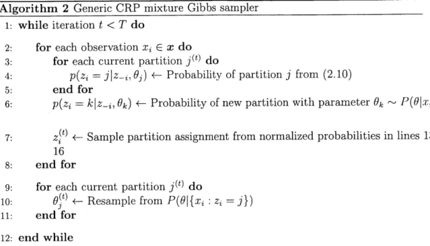
Algorithm 2 outlines the generic Gibbs sampling procedure for the CRP mixture posterior (2.9). Note that the posterior variables to be inferred are sampled separately while others are held constant, i.e. each zi is sampled in Step 17 and each 6O is sampled in Step 10. The assignment sampling in Step 17 of the algorithm relies on the exchangeability of the CRP mixture model by assuming that each xi is the last datapoint to arrive. The posterior assignment probability p(zi =

jI

p(zi =

ijzi,

CRP likelihood

It is assumed that P(Ojx), the conditional of 0 given x, can be sampled.

Given that each sampling update of zi and Oj occurs infinitely often and some mild conditions on the update probabilities are met [60], the resulting samples z)

Algorithm 2 Generic CRP mixture Gibbs sampler

1: while iteration t < T do

2: for each observation xi c x do

3: for each current partition

j(t)

4: p(zi =

jIz-i,

Qj)

j

5: end for

6: p(zi klz-i, Ok) <- Probability of new partition with parameter Ok - P(OI.i)

7: Zt < Sample partition assignment from normalized probabilities in lines

13-16

8: end for

9: for each current partition

j(')

10: 0 <- Resample from P(Oj{xi : zi =

j})

11: end for

12: end while

13: return samples z(1:T) and 0 (1:T), discarding samples for burn-in and lag if desired

and O(t) can be shown to form a Markov chain whose stationary distribution is the target posterior (2.9). In other words, the samples (z(t), 0(t)) will converge to a sample

from (2.9) as t -+ cc.

In practice, for a finite number of iterations T, the chain will be dependent on the initial state of the posterior variables and consecutive samples from the chain will

be correlated (not i.i.d.). To mitigate the effect of arbitrary initial conditions, the

first N burn-in samples are discarded. To mitigate correlation between samples, only every nth lagged sample is kept, and the rest discarded. There is considerable debate as to whether these ad-hoc strategies are theoretically or practically justified, and in general it has proven difficult to characterize convergence of the Gibbs sampler to the stationary Markov chain [75].

Figure 2-1 shows an illustrative example of Algorithm 2 applied to a Chinese restaurant process mixture model where data are generated from 2-dimensional Gaus-sian clusters. In the example, the data x E R2 _{are drawn randomly from five clusters,}

and the parameters to be estimated

0

{p,

unnormal-Posterior Mode, Iteration 0

-x

0 0.2 0.4 0.6 0.8 1 X-coordinate

Posterior Mode, Iteration 15

0 0.2 0.4 0.6 0.8 1 X-coordinate 0.8 .9 0.6 0 0.4 0.2 0

Posterior Mode, Iteration 5

0 0.2 0.4 0.6 0.8 1

X-coordinate

Posterior Mode, Iteration 20

0.8 0.6 0 8 0.4 0.2 0 A0.8 V 0.8 S0.6 0. 72 _'2 0 0 0 0 (30.4 0 4 0.2 0.2 0 0 0 0.2 0.4 0.6 0.8 1 X-coordinate

Posterior Mode Clusters vs. Sampling Iteration

Posterior Mode, Iteration 10

&

Posterior Mode, Iteration 25

0 0.2 0.4 0.6 0.8 1 X-coordinate 10 7 - -6* 0 10 20 30 40 50 80 70 80 90 100

Gibbs Sampling Iteration

Posterior Mode Log Likelihood vs. Sampling Iteration

-15C0 0 -200 -250 -300 -350 *0 -400 -450 o -500 0 10 20 30 40 50 60

Gibbs Sampling Iteration 70 80 90 100

Figure 2-1: Example of Gibbs sampling applied to a Chinese restaurant process mix-ture model, where data are generated from 2-dimensional Gaussian clusters. Observed

data from each of five clusters are shown in color along with cluster covariance

el-lipses (top). Gibbs sampler posterior mode is overlaid as black covariance elel-lipses after 0,5,10,15,20, and 25 sampling iterations (top). Number of posterior mode clus-ters versus sampling iteration (middle). Posterior mode log likelihood versus sampling iteration (bottom). 0.8 A= 0.6 0 0.4 0.2 0 0.8 0.6 0 0 0 0.4 0.2 0 Cn 0 ") 0 0L -DZ)U -. . .. ... .

ized multivariate Gaussian probability density function (PDF), and P(O1x) is taken to be the maximum likelihood estimate of the mean and covariance. Observed data from the five true clusters are shown in color along with the associated covariance ellipses (Figure 2-1 top). The Gibbs sampler posterior mode is overlaid as black covariance ellipses representing each cluster after 0,5,10,15,20, and 25 sampling iterations (Fig-ure 2-1 top). The number of posterior mode clusters (Fig(Fig-ure 2-1 middle) shows that the sampling algorithm, although it is not given the number of true clusters a priori, converges to the correct model within 20 iterations. The posterior mode log likelihood (Figure 2-1 bottom) shows convergence in model likelihood in just 10 iterations. The CRP concentration parameter in (2.8) used for inference is r/ = 1. Nearly identical posterior clustering results are attained for i/ ranging from 1 to 10000, demonstrating robustness to the selection of this parameter.

2.5

Gaussian Processes

A Gaussian process (GP) is a distribution over functions, widely used in machine learning as a nonparametric regression method for estimating continuous functions from sparse and noisy data [72]. In this thesis, Gaussian processes will be used as a subgoal reward representation which can be trained with a single data point but has support over the entire state space.

A training set consists of input vectors X = [x1 ,..., Xn] and corresponding

ob-servations y =[y, ... , y,] . The observations are assumed to be noisy measurements

from the unknown target function

f:

y=

f

where e ~ V(0, af) is Gaussian noise. A zero-mean Gaussian process is completely

specified by a covariance function k(., .), called a kernel. Given the training data

{X,