Artificial gravity as a countermeasure to spaceflight deconditioning : the cardiovascular response to a force gradient

(1)

Artificial Gravity as a Countermeasure to

Spaceflight Deconditioning:

The Cardiovascular Response to a Force Gradient

by

Dawn Hastreiter

Bachelor of Aerospace Engineering & Mechanics, Summa Cum Laude University of Minnesota, 1995

Bachelor of Electrical Engineering, Summa Cum Laude University of Minnesota, 1995

Submitted to the Department of Aeronautics and Astronautics in Partial Fulfillment of the Requirements for the Degree of

Master of Science in Aeronautics and Astronautics

at the

Massachusetts Institute of Technology June 1997

Signature of Author:

Department of Aeronautics and Astronautics May 23, 1997 Certified by:

Professor Laurence R. Young Apollo Program Professor of Astronautics Thesis Supervisor Accepted by:

Professor Jaime Peraire Chair, Graduate Office

(2)

(3)

Artificial Gravity as a Countermeasure to

Spaceflight Deconditioning:

The Cardiovascular Response to a Force Gradient

by

Dawn Hastreiter

Submitted to the Department of Aeronautics and Astronautics on May 23, 1997 in Partial Fulfillment of the Requirements for the

Degree of Master of Science in Aeronautics and Astronautics

Abstract

Before intermittent short-arm centrifugation can be tested as a countermeasure to space deconditioning, a number of ground-based studies must be conducted to determine the effects of a gravity gradient both on normal subjects and individuals undergoing bed rest. This investigation focused on determining several of the cardiovascular effects of a gravity gradient on normal subjects. The purposes of the investigation were to answer the following questions: 1) how cardiovascular performance measures change with G level and duration of stimulation, 2) how do cardiovascular parameters change during force gradient stimulation as compared to their response to standing in 1 G, and 3) what levels of force gradient stimulation promote significant cardiovascular regulation? It was hypothesized that G levels of 1 and less at the feet would produce few cardiovascular changes in normal subjects. This investigation will enable future researchers to more precisely outline centrifuge studies necessary on individuals undergoing bed rest treatments as models for spaceflight deconditioning. The hope is that a SAC may someday be used in space to keep the cardiovascular system stimulated to minimize orthostatic intolerance.

Eight subjects, four men and four women, participated in one control and three rotation tri-als on a horizontal short-arm centrifuge (SAC) such that the Gz levels at the feet were 0.5, 1.0, and 1.5. Trials consisted of 30 min. of supine rest, 1 hour of rotation (or in the control, 30 additional min. of rest and 30 min. of standing), and a final 30-minute rest period. Measurements of heart rate, calf impedance, calf volume, and blood pressure were obtained. Post-trial analysis explored the relationships between the physical characteristics of the subjects, rotation time, G level, and the cardiovascular parameters measured. Most measured cardiac parameters suggest that rotation levels causing 1.0 G at the feet or less produced regulatory responses not significantly different from continued supine rest. In addition, the cardiovascular responses to SAC rotation with 1.5 G at the feet were statistically similar to standing, at least for a comparison based on 30 min. The primary effects of 1.5 G were an elevated diastolic pressure, increased heart rate, and increased calf volume. While some cardiovascular changes were found to be correlated to gender, mass, and height, their influence was considered minor. Most importantly, since standing intermittently during bed rest trials has been shown to decrease orthostatic intolerance and rotation at 1.5 G was found here to be similar to standing, short-arm centrifugation should be considered as a possible countermeasure to cardiovascular space deconditioning. Rotation durations on the order of 30 min. may be required for promotion of sufficient cardiovascular regulation in inactive subjects.

Thesis Supervisor: Dr. Laurence R. Young Title: Apollo Program Professor of Astronautics

(4)

(5)

Acknowledgments

Funding for this work was provided by NASA Grant NAGW-3958, the MIT Man-Vehicle Laboratory, and the Department of Defense (U.S. Air Force) Graduate Fellowship Program.

The following members of the MIT community participation in this research:

Albert Assad, M.D. Steve Burns, Ph.D. Richard Cohen, M.D., Ph.D. Catherine Coury Peter Diamandis, M.D. Mark Davies Kristen Fisher Barbara Glas Keoki Jackson, Ph.D. Minh Le Robert Lees, M.D. Mike Markmiller Thomas Mullen, Ph.D. Alan Natapoff, Ph.D. Matt Neimark Dava Newman, Ph.D. Charles Oman, Ph.D.

are to be thanked for their advice, aid, or

Richard Perdichizzi Emerson Quan David Rahn Scott Rasmussen Jennifer Rochlis Teresa Santiago Javorka Saracevic Patricia Schmidt Lisa Shimizu Prashant Sinha Adam Skwersky Anna Tomassini Christine Tovee Michail Tryfonidis Donald Weiner Elise Westmeyer Laurence Young, Sc.D.

The following members Jay Buckey, M.D. David Cardd's, M.D. John Greenleaf, Ph.D.

of the NASA community are to be thanked for their advice in this research: Alan Hargens, Ph.D.

Joan Vernikos, Ph.D.

Special gratitude goes to the following persons and their institutions for the loan of laboratory equipment necessary for this research:

Allied Signal, Inc. -- Blood pressure monitor

Dr. Richard Cohen, MIT Division of Health Sciences and Technology -- ECG Dr. Steve Bums, MIT Division Health Sciences and Technology -- ECG

(6)

(7)

List of Figures

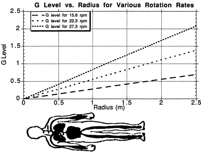
Figure 1. Variation of Gz level Along a Body with Radius and Rotation Rate...17

Figure 2. Pressure Gradients Induced by Orthostatic Stresses...19

Figure 3. The Cardiovascular Response to Short-Arm Centrifugation in Carddis's Study ... 22

Figure 4. Subject on the MIT-Artificial Gravity Simulator (AGS) ... 24

Figure 5. The MIT-Artificial Gravity Simulator (AGS)...26

Figure 6. Stimulation Profiles for Trials...27

Figure 7. Minnesota Impedance Cardiograph... 29

Figure 8. Example of Impedance Leads and Circumference Lines ... 29

Figure 9. Example Calf Profile and Curve Fits...31

Figure 10. Example of Filtering of ECG Signals...33

Figure 11. Impulse Responses of the ECG Filter ... 34

Figure 12. Normalized Calf Impedance Data for Subject J...39

Figure 13. Calf Impedance Data...40

Figure 14. Calf Volume Data...44

Figures 15a-c. Plots for Assessing the Relationship Between Calf Impedance and Volume...46

Figures 16. Average, Normalized Blood Pressure Results for the 4 Trials ... 47

Figure 17. Average, Normalized Systolic Blood Pressure Results for the 4 Trials ... 48

Figure 18. Average, Normalized Diastolic Blood Pressure Results for the 4 Trials... 49

Figure 19. Examples of R-R Interval and Instantaneous Heart Rate Plots ... 53

(10)

List of Tables

Table 1. Space Adaptation Syndrome Effects...13

Table 2. Questions Regarding the Physiological Requirements for Artificial Gravity...15

Table 3. Biometric Characteristics and Rotation Parameters of the Subjects ... 27

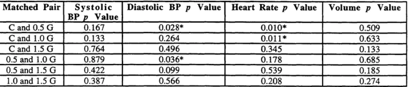
Table 4. p Values for Comparisons Between Resting Values of the Different Trials...36

Table 5. Statistics for Comparisons Between the Resting Cardiovascular Parameters Between M ale and Fem ale Subjects...37

Table 6. Significant Correlations Between Experimental Results and Subject Resting CV Parameters and Biometric Characteristics ... 38

Table 7. p Values for Impedance Comparisons Between the Trials ... 42

Table 8. p Values for Impedance Comparisons Within the Trials ... 43

Table 9. p Values for Volume Comparisons Within the G Trials...45

Table 10. p Values for Blood Pressure Comparisons Between the Trials ... 50

Table 11. p Values for Blood Pressure Comparisons Within the Control Trial...51

Table 12. p Values for Blood Pressure Comparisons Within the 0.5 G Trial...51

Table 15. p Values for Heart Rate Comparisons Between the Trials...55

Table 16. p Values for Heart Rate Comparisons Within the Trials ... 56

(11)

We are the children of gravity. We can't touch it or see it. But it has guided the evolutionary destiny of every plant and animal species, and has dictated the size and shape of our organs and limbs. Every bone and muscle is aligned to maximize mobility in 1 G.

(12)

(13)

INTRODUCTION

The Case for Artificial Gravity

Living in a weightless environment often produces physiological changes referred to as space adaptation syndrome (SAS). The effects of SAS have been well documented (Grymes 1995; Convertino and Sandler 1995), and generalized symptoms are listed in Table 1 (Sander, et al. 1995). Changes in the skeletal and cardiovascular systems are particularly alarming. 1-2% of bone mass is lost per month in space (Sandler 1995). This is a critical problem affecting long-term spaceflight. Issues related to loss of orthostatic tolerance are also of concern. Astronaut faintness during reentry or during an emergency landing on earth or another planet is a real danger caused by cardiovascular deficiencies.

Table 1. Space Adaptation Syndrome Effects

Anorexia Decreased Exercise Capacity

Nausea Muscular Incoordination

* Motion Sickness Muscle Atrophy

* Disorientation Fluid Shift

Restlessness Dehydration

Sleeplessness Weight Loss

Fatigue * Gastrointestinal Disturbances

Lethargy Renal Calculi

Immune System Degradation Reduced Plasma Volume

* Demineralization of Bones Reduced Blood Volume

* Loss in Bone Mass * Cardiac Arrhythmias

Spine Length Increase/Pain Tachycardia

* Decreased G Tolerance Hypertension

* Postflight Syncope * Hypotension

* May cause an emergency situation in flight.

Current countermeasures against SAS include exercise, the Russian Penguin suit, fluid loading, diet modification, lower body negative pressure (LBNP), preflight adaptation training, drugs, and electrical muscle stimulation. The primary inflight exercises practiced in the Russian and American space programs are use of a cycle ergometer, running on a treadmill, and resistance training. These maintain aerobic capacity and do a somewhat sufficient job of maintaining muscular strength. Similar to the exercise training is the Penguin suit, an elasticized garment that requires extra force to be exerted for normal movements. Fluid loading in-flight corrects for plasma volume loss and helps prevent disorders such as renal stone formation (Heer, et al. 1995). Fluid loading prior to reentry is intended to help maintain orthostatic tolerance during the large reentry G forces (up to 2 G). The potential of diet modification as a countermeasure has not fully been explored, but it can only attenuate some of the effects of SAS. Current ground-based

(14)

research on the use of LBNP is showing promise (GUell 1995); however, few in-flight studies of LBNP as a countermeasure to orthostatic intolerance have proven its effectiveness. At the moment, preflight adaptation training may consist of occasional flights in the KC-135 (to experience 0 G), underwater training, acceleration G profiles similar to Shuttle launch, and exposure to disorienting vestibular stimuli in the JSC Pre-Adaptation Trainer. However, a formal preflight adaptation program does not exist. No psychological preflight training is currently practiced either. Promethazine, for motion sickness, is the most advanced pharmacological countermeasure in place today. Altered pharmacokinetics and pharmacodynamics in microgravity have prevented most drug treatments available on Earth from being applied as countermeasures to SAS in space (Vernikos 1995). Electrically stimulating the muscles has been practiced for years by the Russians to prevent atrophy and has met with some success (Convertino and Sandler 1995).

While current countermeasures attack many aspects of space deconditioning, not one preserves bone density. Orthostatic tolerance and muscular strength are not totally sustained either. Russian cosmonauts have made extensive use of the Penguin Suit and exercise countermeasures for durations longer than one year, but they cannot walk unassisted for at least 48 hours after landing. Russell Burton, Chief Scientist at the U.S. Air Force School of Aerospace Medicine (USAFSAM), stated the problem nicely when he said (1989), "The Occupational Safety and Health Association would probably not allow employees to work in such a hazardous environment on earth, so why should it be permitted in space?" The failure of existing therapies for dealing with the debilitating effects of long duration weightlessness may call for artificial gravity (AG) as the only way to prevent SAS.

Why do we need something as extreme as artificial gravity (AG) when we can allow the astronauts to recuperate when they return? That question may be valid for short-term flights and even space station missions, but for long-term explorations such as a Mars venture certain additional considerations merit use of the extreme countermeasure. Current technology dictates that a Mars trip will require at least two years in microgravity because "the diverse capabilities of such energy sources as the dilithium crystals used on the U.S.S. Enterprise are as yet unavailable to NASA" (Grymes 1995). Providing astronauts with AG on the trip to Mars could produce several benefits. The gravity level of Mars is only 37.5% of Earth's. No one has ever lived in microgravity for one year and returned to a gravity environment without medical treatment available. AG would maintain the astronauts' ability to perform emergency extravehicular activities (EVA's), prevent bone fractures, and maintain the pilots' ability to perform their duties. Also, adaptation time to the Mars environment might decrease if 0.375 G could be provided prior to a Mars landing. Thus, few of the precious days on Mars would be wasted due to astronauts' limited functionality. Finally, it is not inconceivable that someday humans will live in space for many

(15)

environment of the moon (0.16 G) or Mars are unknown. AG may need to be provided even on the surface. The challenge is to determine what kind of AG (what G level and for how long in the context of this paper) is necessary in any of these situations.

Performing AG research has been difficult at best because the human 1 G requirements are unknown and all experiments on Earth are subject to a 1 G force. Critical studies that have been conducted pertaining to the physiological effects of AG are summarized in Appendix A. They are categorized according to the rotation environment or purpose of study. Some general observations can be made. Most of the experiments were conducted long before acquisition of the current knowledge of SAS. Usually, a handful of subjects were tested, making the validity of the findings questionable. In addition, many of the tests were not comprehensive and varied considerably so that comparisons are nearly impossible. Still, the results of these studies, the fact that bed rest can approximate the physiological effects of microgravity exposure (for some but not all major body systems), and recent orthopedic research indicate that it is not just the G force that maintains the human system but the activities carried out in the G force (Schneider, et al. 1993). That different activities stimulate different body systems seems to be clear as well. The conclusions of the intermittent stimulation investigations, added to the knowledge that humans sleep horizontally each night with no ill effects, imply that humans do not require constant exposure to gravity along the vertical axis of the body. As a final observation, each of the studies in Appendix A is concerned with only a specific aspect of AG, usually intermittent or constant exposure. While some

suggestions have been made (Kotovskaya, et al. 1977; Workshop on the Role of Life Science in

the Variable Gravity Research Facility 1988; Burton 1989), an overall research approach to

determine the physiological AG requirements for long-term spaceflight is decidedly absent.

Before deciding what research is necessary to determine the physiological requirements for AG, a comprehensive set of questions must be compiled. As complete a list as possible is shown in Table 2. Note that only questions necessary to provide AG for long-term spaceflight are listed. Many more could be added if the entire physiological response to force levels were desired. These questions include those that must be answered for both AG provided by a rotating spacecraft and AG provided by a short-arm centrifuge (SAC) in a nonrotating spacecraft.

Motivation

As mentioned previously, one of the methods of providing artificial gravity to astronauts is by using short-arm centrifugation in space. This would most likely occur via intermittent stimulation on a SAC since a space crew would not be likely to live and work in a small volume, as would be the case if short-arm centrifugation were applied by spinning the entire spacecraft. Before a SAC can be tested as a countermeasure in space, a number of ground-based studies must

(16)

be conducted to determine the effects of a gravity gradient both on normal subjects and individuals undergoing bed rest, a treatment that mimics microgravity exposure.

Table 2. Questions Regarding the Physiological Requirements for Artificial Gravity

1. How much time in 1 G is necessary to maintain normal physiological status?

2. What activities in 1 G keep humans fit?

3. Since the activities we perform in a gravitational field stimulate us, then passive exposure to

rotational G during sleep is of little benefit. Is there a best time of day to provide 1 G?

4. Should 1 G be provided in a lump sum or intermittently during a day?

5. If exposed to the microgravity environment for a period of time, how long does reconditioning via AG take, or can it be done at all?

6. Does exposure to G levels greater than 1 decrease the total stimulation time?

7. What the relationship between the steady-state physiological response and the G level? 8. What is the character of the physiological transient response to a G level?

9. What is the relationship between the G-level physiological response and age, gender, fitness,

etc.?

10. What is the physiological response to a G gradient along the body?

11. The effects of motion sickness caused by angular cross-coupling in a rotating environment on

the general body system can be determined by comparing the response of subjects who have lost vestibular function to that of normal subjects. After this knowledge is gained, how can it be applied to reduce the severity of or eliminate the detriments of rotational motion sickness in a normal person?

12. Does the Coriolis stimulation of the rotating environment affect physiological responses?

13. What is the best way to adapt to a rotating environment?

14. Burton cites data implying that animals can adapt to increased G environments while maintaining adaptation to 1 G (1989). Can a human maintain adaptation to two G levels for a period of time without experiencing major side effects from transition between the two levels?

15. If partial gravity could only be provided because of engineering/cost concerns, how much more stimulation time is necessary, or can partial gravity exposure be beneficial at all?

16. How similar are adaptation and physiological responses to a rotating environment on earth to

those caused by a rotating environment in space?

This investigation focused on determining several of the cardiovascular (CV) effects of a gravity gradient on normal subjects. Specifically, one purpose of the investigation was to determine how cardiovascular performance measures change with G level and duration of stimulation. Additional questions considered were: (1) how do cardiovascular parameters change during force gradient stimulation as compared to their response to standing in 1 G, and (2) what "safe" levels of force gradient stimulation promote significant cardiovascular regulation? In essence, partial answers to questions 7-10 in Table 2 were sought. As a result of previous research in this area and physical principles, it was hypothesized that G levels of 1 and less at the feet would produce few cardiovascular changes in normal subjects.

(17)

The added benefit is increased knowledge about gravitational physiology. The hope is that a SAC may someday be used in space to keep the cardiovascular system stimulated to reduce the likelihood of orthostatic intolerance, among other effects.

Background

G Level vs. Radius for Various Rotation Rates

2 =

I

2 n

.

0-

-.5

11.5

2

2 Radius (m)

Figure 1. Variation of Gz Level Along a Body with Radius and Rotation Rate

A consequence of short-arm centrifugation is a force, or gravity, gradient along the body. Centrifugal acceleration, a, obeys the law

a=rO

2 1

where w is angular velocity and r is the radius. Thus, a body subjected to a constant angular velocity on a SAC will experience a different force at each location along its longitudinal, or z,

axis. The following equation can be used to calculate G level, were w is in rpm and r is in meters:

ro( 27r rad

y

1min 2

[1

rev

A60

sj

G level= (2) 9.81 M/s2 G evel for 15.8 rpm I G evel for 22.3 rpm Gjleve for 273rpm .. ... ... ... .. .. .. .. .. .... .. . . . .-.. . . . . Sew. S 00,10 .. ~...,.. .9 * 00

(18)

Figure 1 displays curves for G level along a body for various angular rotation rates. As specified by question 10 in Table 2, the effect of the variation in force on humans has not been completely characterized.

Obviously, no centrifuge on Earth can subject a body to less than 1 G in three-dimensional space. Rather, a centrifuge rider is subjected to the vector sum of the centrifugal force and Earth's gravity. In general, studies conducted on centrifuges refer only to the G level along the rotation radius. In addition, since a force gradient exists, experimenters often refer to the G level in SAC studies as being the force felt at the feet. For example, a rotation rate of 22.3 rpm will cause a G level of 1 at the feet of a 1.8 m person whose head is placed at the center of rotation. The same rotation rate will only produce 0.80 G in a person 1.5 m tall whose head is at the center of rotation as well. The force component felt through the x-axis of a supine person, gravity, is generally considered of negligible importance to the results (of studies such as the present where subjects are horizontally supine) because the height of the x-axis hydrostatic column is small compared to the z-axis column and most major systemic blood vessels are aligned with the body's z-z-axis (Breit, et al.

1996).

Standing under the influence of normal gravity creates a pressure gradient along the z-axis of the body. The normal hydrostatic pressure relation is given by

P=pgz+P,, (3)

where p is density, g is normal gravitational acceleration, z is the height from a reference level, and

P0 is the reference pressure. For rotation on a centrifuge the pressure relation becomes

P=4p92(z2 - z2)+., (4)

with z now representing the distance along the radius. If the heart is considered to be at the reference level, with a mean arterial pressure of 100 mmHg, then Figure 2 compares the pressure gradients induced by standing and rotation at 0.5, 1.0, and 1.5 G in a 1.8 m person. While supine, the arterial pressure over the body is much more uniform than any of the curves in Figure 2.

Before discussing the mechanisms responsible for orthostatic intolerance and how to prevent the condition, several CV variables and relations should be defined. Cardiac output (CO) is the volume of blood pumped out of the heart per unit time. It is calculated by

CO = SV x HR, (5)

where HR is the heart rate and SV is the stroke volume, the volume of blood pumped out of the heart with each beat. The pulse pressure, PP. the difference between and systolic and diastolic pressures, can be directly related to SV through

PP SV ₍₆₎

(19)

Pressure vs. Distance Along the z-Axis of the Bod'

200---- Standing -0.5 G 1

8 - -.. - - - 1.0 G

... ... ... ...,I ... --- 1.5 G-1 6 - ... .... ... ... ... ... ... , ... ... ... .

E 1 64 0

---

----

--- ---

----

-

-E

160-...

... ... .... .. ...

.--

MM... ... 1 2 0 -- - --- - - -

-+---CA

140-0

omow 1

12

0 7 . ... ...---... 8 0) --- ... -- 60 1

0

0.45

0.9

1.35

1.8 z

(m)

Figure 2. Pressure Gradients Induced by Orthostatic Stresses

Calculations are based on a 1.8 m person with the heart located 0.45 m from the top of the head. The curves were produced assuming 100 mmHg was the pressure in the heart for comparison purposes. However, centrifugation normally raises the mean arterial pressure above 100 mmHg.

where Ca is the arterial capacitance. Unlike SV, Ca is a relatively invariant to stresses induced on the body. Generally, one of the fundamental functions of CV regulation is to maintain cardiac output at a level sufficient to sustain perfusion to the brain and to maintain pressure in the circulatory system. Mean arterial pressure can be found using

(20)

F=lp -9 PD, (7) where PS is the systolic pressure and PD is the diastolic pressure.

Alterations in posture or the gravity environment create increased pressure in the lower body which leads to venous pooling in legs. A postural example that demonstrates this is the transition to standing after being supine for a period of time. Hypergravity conditions will also cause venous pooling. If the increased blood flow to the periphery is not regulated, venous return to the heart is impeded. This leads to decreased cardiac output, decreased blood pressure, and eventual syncope, the classic sign of orthostatic intolerance. Orthostatic tolerance is normally maintained by compression of leg veins through local regulation and baroreflex-mediated sympathoexcitation and vagal withdrawal.

The primary mechanisms related to cardiovascular responses to orthostatic stress that will be discussed here are autonomic control of the cardiovascular system and the baroreflex response. For a further discussion of CV regulatory mechanisms the reader is referred to Blomqvist (1983) or Churchill and Bungo (1997). Autonomic control of the CV system is mediated by sympathetic and parasympathetic innervation. The parasympathetic system innervates the heart via the vagus nerve and acts to reduce heart rate. In the context of the present experiment, activation of the sympathetic system increases heart rate, increases contractility of the heart, and causes vasoconstriction. The arterial baroreflex is a mechanism for regulating arterial pressure by sensing pressure in the arteries and responding with changes in control of cardiac output or peripheral resistance to achieve a desired CV set-point. The pressure sensors, termed baroreceptors, are found in the aortic arch and a region of the neck called the corotid sinus. In the case of the present study, the barorecptors will sense a decrease in arterial pressure when the body transitions from supine rest to an orthostatic stress. The baroreceptors will then normally cause the following changes, among others, to occur: a decrease in vagal activity, an increase in sympathetic activity to all portions of the CV system, arteriolar and venular vasoconstriction (increasing total peripheral resistance), and an increase in heart rate.

When astronauts return to the gravity environment of Earth from a stay in space, the cardiovascular regulatory mechanisms that prevent excessive blood pooling in the legs do not function properly. It is for this reason that 9 to 64% (depending on the particular study) of astronauts fail a 10 min. standing test after return to Earth (Buckey, et al. 1996). According to recent studies, the major hemodynamic defect related to orthostatic intolerance resulting from spaceflight is a lack of vasoconstriction in the lower limbs (Buckey, et al. 1997). Total peripheral resistance does not rise adequately. Changes in the baroreflex sensitivity have not been confirmed (Arbeille, et al. 1997; Buckey, et al. 1996) so sympathetic circulatory control alterations are suspect. In a simplified explanation, current theory believes these alterations in the CV regulatory system occur as a result of disuse in space. In a sense, the CV reflexes "have not been practicing."

(21)

It has been suggested that standing intermittently could be an effective countermeasure to the orthostatic intolerance seen in SAS (Vernikos 1994). A study was performed in which subjects were exposed to four days of -6' head-down bed rest interrupted by 15-minute periods of standing. Two conditions, standing 8 times per day (2 hours total) and standing 16 times per day (4 hours total), were tested. Orthostatic tolerance was assessed by 30 min. of 60' head-up tilt. Presyncope indicated failure of the test. Standing 8 times per day partially prevented and standing 16 times per day completely prevented orthostatic intolerance. To stand in space, a gravity field would need to be created. This paper investigates SAC rotation as the mechanism for providing the gravity field.

Several studies have investigated the effects of a gravity gradient on the cardiovascular system. Shulzhenko and Vil-Viliams (1992) monitored the orthostatic intolerance during 3-day dry immersions (another analog of microgravity exposure) of 4-6 subjects who were intermittently exposed to rotation on a 2 m-radius centrifuge. Orthostatic function was assessed by time tolerance to rotation on a 7.25 in centrifuge at +3 Gz. In one study, subjects experienced 40-60

min. of 0.8, 1.2, or 1.6 G two to three times daily. As compared to pre-dry immersion, orthostatic tolerance decreased 18%, 7%, and 1%, respectively, at the end of the three days. The control decrease was 21%. When water and salt supplements were added and the experiment was repeated for the 0.8 and 1.2 G levels, the orthostatic tolerance only decreased 7% and 1%, respectively. The same experimenters conducted a 28-day trial with the following time profile: 7 days of no-exposure dry immersion, 7 days with 40-60-minute blocks of 0.8, 1.2, or 1.6 G 2-3 times daily, 7 days with periodic supine bicycle ergometer training, and 7 days with SAC rotation combined with bicycle ergometry for 60 min. twice daily. It was found that after the first 7 days, orthostatic tolerance had decreased by 56%. After 28 days, orthostatic tolerance was 8% less than normal. While this last experiment clouds the issue because of the combined interventions, the combination of the three trials proves that rotation at hypergravity attenuates loss of orthostatic tolerance due to physiological microgravity analogs.

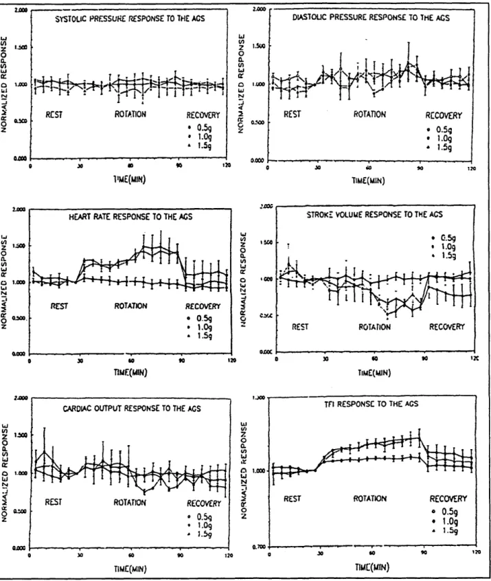
Cardiis (1993a, 1993b) performed a study on six men with measurements of general cardiovascular signals for one hour durations on a 2 m-radius SAC. G levels of 0.5, 1.0 (with only 3 subjects in this case), and 1.5 at the feet were tested. Time profiles for the trials included a 30-minute supine rest period, one hour of rotation, and a final 30-minute rest period. The experimenters observed few cardiovascular changes for G levels below 1 at the feet. Cardiovascular alterations did occur for G levels in the 1-1.5 range. Above 1.5 G, cardiovascular changes became more dramatic, with 2 G inducing syncope in some subjects. Figure 3 displays some of the results of the experiment for three rotation rates. It should be noted that the authors used rates of 17, 20, and 24 rpm to produce estimated G levels of 0.5, 1.0, and 1.5 G. Rotation rates were not adjusted for subject height. No statistical comparisons were performed although it

(22)

SYSTOLC PRESSURE RESPONSE TO THE ACS. DASIOUC PRESSURE RESPONSE TO THE ACS

REIRaTJ RCVEY URSTRTTONR~vR

1 .. g .5.0

0 0

it~uN iN TTME(

J0 0.5

ROTATION RECOVERY 2 REST ROTATION RECOVERY

. 0.5g 0 0 1.09 - EEOE £ 1.59 _A_1.5g o a 220 i so 12C 'ME(MIII) TIME(MIN) 2=00

HEART RATE RESPONSE TO THE AGS STROKE VOLUME RESPONSE ro THE AGS

1 A 0.59 0 Z 0 1.09 0 _1.5g kL TUM(M wT - (IN WI W

REST ROTATION RECOVERY

Z * I.09 REST ROTATION RECOVERY

a1.59

R so t d 0 b 120 f0 s t t t r s

TIMEQMIN) TimE(MIN)

CARDIAC OUTPUT RESPONSE TO THE AGS TFI RESPONSE TO THE AS

V) U)

0 0r

(L 0.

o 1.00 1.000.

NJ N

R<AINRCVR REST ROTATION RECOVERY

ox 0=~ 0 * 0.59

z01.09 * 1.Og

& 1.59 1.59

o 060 60 120 0 J 60 0 20

TiME(MIN) TIUEQ(ffN)

Figure 3. The Cardiovascular Response to Short-Arm Centrifugation in Cardis's Study

Results of experiments conducted by Cardus (1993b) for 6 male subjects at three rotation rates. (Only three subjects participated in the middle rotation rate trial). Trials consisted of 30 min. rest, 1 hour of rotation, and a final 30-minute rest period. Rotation was performed on a SAC termed the Artificial Gravity Simulator (AGS). TFI = thoracic fluid index

(23)

was noted that diastolic pressure tended to increase slightly. In addition, data were not compared to continued supine rest substituted for rotation. From Figure 3, one can see that systolic pressure changed little and diastolic pressure showed some increase as the rotation rate was raised. Heart rate increased and stroke volume decreased for the 1.0 and 1.5 G cases. Careful study shows that after the initial change in these two parameters, a small recovery took place, followed by a much larger alteration occurring at approximately 30 min. The thoracic fluid index (TFI) was measured via electrical impedance. An increase in impedance (or TFI) corresponds to a decrease in volume over the area measured. The plots show that TFI increased with rotation, especially at the higher G levels. This can be interpreted to mean that fluid was transferred from the thoracic cavity to the lower body. Note that this effect does not reach steady state in the one hour of rotation for the higher G levels.

Researchers at NASA Ames Research Center (Breit, et al. 1996) also conducted a study on eight men and seven women to compare the effects of short-arm centrifugation (with a 75% Gz gradient), long-arm centrifugation (with a 25% Gz gradient), whole-body tilting, and lower body negative pressure on regional cutaneous microvascular flow, mean arterial pressure, and heart rate. Stimuli were applied for only 30 s at a time, and transitions between stimuli levels were performed in 10 s without stopping the stimulus. Their investigation was limited to G levels of 1 and below (0.2, 0.4, 0.6, 0.8, and 1.0) at the feet. LBNP was found to cause the greatest relative flow reduction in the lower body. All stressors except short-arm centrifugation resulted in an increased heart rate. Head-up tilt was the only orthostatic stressor which produced a change in mean arterial pressure. The experimenters found no correlation between height and gender and the cardiovascular responses to centrifugation. Centrifugation was also found to produce the least severe vasoconstriction. Their results showed flow inconsistency among the subjects when exposed to centrifugation as opposed to the other orthostatic stressors. Vestibular stimulation was suggested a possible explanation. The experimenters concluded that centrifugation, especially using a SAC, may be disadvantageous for baroreflex stimulation because the carotid sinus is near the top of the pressure column and because they observed little heart rate change in their study.

The goals of the studies mentioned above and of the present experiment are to determine what stressors cause cardiovascular regulation sufficient enough to keep the CV system in practice. This paper details an investigation of short-arm centrifugation as a method for CV stimulation. Rotation trials at 0.5, 1.0, and 1.5 G were conducted for one-hour durations with pre- and post-stimulus supine periods. Since standing has been proposed as a countermeasure to SAS-in uced orthostatic intolerance, responses to iotation were compared to those that standing produces to determine if adequate stimulation is caused by SAC rotation.

(24)

(25)

METHODS

General

The rotation research was conducted using the MIT-Artificial Gravity Simulator (AGS) (Massachusetts Institute of Technology Man-Vehicle Laboratory), pictured in Figures 4 and 5, a 2 m-radius rotating platform with the ability to exceed 30 rpm (Diamandis 1988). Modifications to the AGS can be found in another document (Tomassini 1997). Rotation rate, subject position, and mounted physiological monitoring equipment were variable for the AGS. Subjects were placed supine on the AGS, such that the tops of their heads were at the center of rotation (made possible by the AGS's adjustable foot plate). As seen in Figure 4, the AGS is covered by a transparent (so that the experimenter could easily view the subjects) wind canopy, to prevent cooling of the subjects from wind. Linen material loosely sealed both ends of the canopy. Rotation rate was determined via a tachometer mounted on the motor (seen immediately below the AGS platform and mid-picture in Figure 4). The AGS tended to increase rotation speed as time progressed, so manual feedback was employed to maintain a constant angular speed. A video camera (Sony # PVM-122), as seen in Figure 5, was available for viewing the subjects and physiological

monitoring equipment. The floor of the AGS platform and the foot plate were padded with foam for subject comfort. An emergency stop button, with the ability to stop the rotator in 15 s for G levels up to 1.5, was available for both the experimenter and subject. Rotation was commenced at a rate of less than 1 rpm/s. Generally, the target rotation rate was achieved 30 s from rotation onset.

This experiment was approved by the MIT Committee on the Use of Humans as Experimental Subjects. Appendix B contains the COUHES application, subject consent form, and subject selection questionnaire. Experimental participants were required to be in good health, have no cardiovascular abnormalities, and not to be pregnant. Subjects were asked to abstain from caffeine and alcohol intake 24 hours prior to each experimental session. In later trials, subjects were asked if they had eaten well, how much sleep they had had, and if they had taken any medications prior to each experiment. Subjects were blindfolded to prevent motion sickness induced by conflicting vestibular-visual cues. They were also instructed to move as little as possible. This was especially true while blood pressure measurements were being taken. It was made imminently clear that any head movements would induce motion sickness and would be counter-productive to the experiment. The experimenter and subject were in continuous two-way communication via radio headsets (Voice-Operated 49 MHz Two-Way Communication System, cat. no. 21-406, Radio Shack). To prevent the subjects from falling asleep, the experimenter read to them, talked with them, and played music during rest periods.

(26)

(27)

Stimulation vs. Time _{Figure 6 shows the stimulation profiles} standing for the four trials. Rotation trials included a

30-minute supine rest period, 1 hour of rotation, and a final 30-minute supine rest

s speriod (with the exception of the 1.0 G trial for

rotaton _{subject D in which only 25 min. of rest}

followed rotation). Each subject participated in supine rest supine rest three rotation trials, otherwise termed G trials, such that the G levels at the feet during rotation

0 15 30 45 60 75 90 105 120 were 0.5, 1.0, and 1.5. Table 3 shows the

Time (min) _{rotation rates, calculated from Equation 1, that}

Figure 6. Stimulation Profiles for Trials _{were required for each subject to produce the} appropriate G levels at their feet. A control trial for each subject was performed before the rotation trials, involving 1 hour of rest, 30 min. of standing, and a final 30-minute rest period. For each subject, only one trial was performed per day, all four trials were completed within 1.5 weeks, and the time of day of experimentation was controlled to within one hour. The protocol checklist is presented in Appendix C. Subjects performed the rotation trials in a pre-determined, semi-random order. The order for each subject is shown in Table 3. Because only eight subjects were studied and it was desired to have one man and one woman perform the same trial order, a full Latin square randomization of rotation trials could not be fulfilled. Since 1.0 and 1.5 G were likely to produce the greatest effects, it was decided to have these two levels as the two initial rates available in the partial Latin square. Subjects were not told how much time had elapsed during the trials nor were they told what G level they were experiencing.

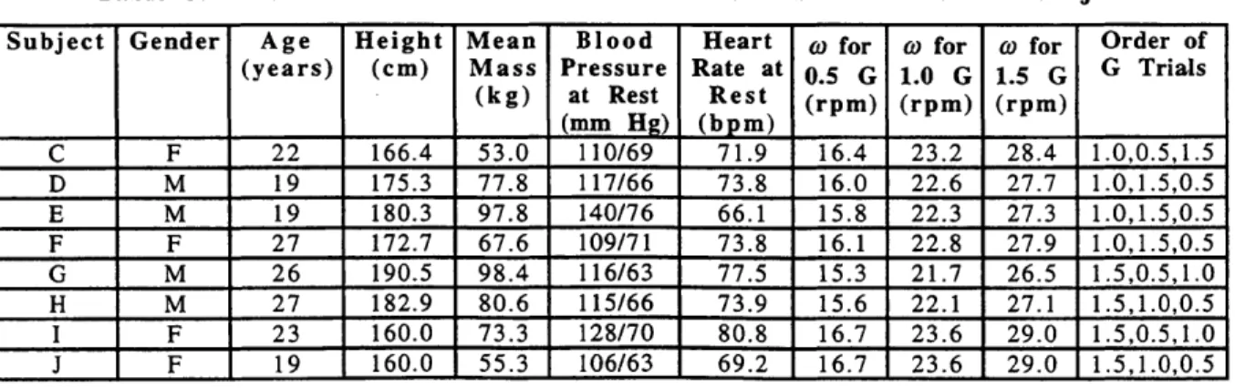
Table 3. Biometric Characteristics and Rotation Parameters of the Subjects

Subject Gender Age Height Mean Blood Heart w for (o for o for Order of (years) (cm) Mass Pressure Rate at 0.5 G 1.0 G 1.5 G G Trials

(kg) at Rest Rest _{(rpm) (rpm) (rpm)} (mm Hg) _(bpm) C F 22 166.4 53.0 110/69 71.9 16.4 23.2 28.4 1.0,0.5,1.5 D M 19 175.3 77.8 117/66 73.8 16.0 22.6 27.7 1.0,1.5,0.5 E M 19 180.3 97.8 140/76 66.1 15.8 22.3 27.3 1.0,1.5,0.5 F F 27 172.7 67.6 109/71 73.8 16.1 22.8 27.9 1.0,1.5,0.5 G M 26 190.5 98.4 116/63 77.5 15.3 21.7 26.5 1.5,0.5,1.0 H M 27 182.9 80.6 115/66 73.9 15.6 22.1 27.1 1.5,1.0,0.5 I F 23 160.0 73.3 128/70 80.8 16.7 23.6 29.0 1.5,0.5,1.0 J F 19 160.0 55.3 106/63 69.2 16.7 23.6 29.0 1.5,1.0,0.5 For the control trial, subjects performed the supine portions on the AGS. They were allowed to sit up approximately 20 s prior to standing. The experimenter aided them in the

(28)

transition from the AGS to standing. While standing, subjects positioned their back against a wall but were allowed to place their feet naturally (as long as the angle the legs made with the wall was not too great). They were allowed to make minor movements of their legs such as shifting weight but were not required to "stand at attention." The experimenter remained at the side of the subject at all times to observe any presyncopal symptoms.

Four male and four female healthy volunteers, coded C-J, provided written consent to participate in this study, comprised of four trial sessions. The subjects had the following physical characteristics (mean ± standard deviation): age = 22.75 ± 3.6 years, height = 1.74 ± 0.11 m, mass = 75.5 ± 17.0 kg, resting blood pressure = 118/68 + 11/4 mm Hg, and resting heart rate =

73.4 i 4.6 bpm. Table 3 displays the individual biometric statistics for the subjects. The mean mass was the average of the masses measured on each of the four trial days. The maximum coefficient of variation for mass was 1.7%.

Calf Impedance and Volume

Calf impedance (I) was measured at 0.2 Hz with a Minnesota Impedance Cardiograph (Model 304B), pictured in Figure 7. The impedance cardiograph was utilized as an impedance plethysmograph in this experiment. Four circumferential electrical leads, as seen in Figure 8, were attached to one leg of a subject, two near the ankle and two near the knee. The leads were formed by wrapping electrode tape (Cardiograph Electrode Tape, IFM T-8001, Instrumentation for Medicine, Inc.), with electrode gel (Signa Gel, # 0341-15-25, Parker Laboratories, Inc.) applied to the electrode portion, around the limb and meeting the two ends. The impedance cardiograph leads were then clipped to the joined ends of the tape. Subjects were not required to remove hair from their calves. At times the electrode tape did not stick properly; so medical tape (Kendall Tenderskin Hypoallergenic Paper Tape, # 1914) was employed to improve attachment. The two outer leads ran a 4 mA AC current between them. The inner two leads measured the mean resistance (ZO = I) of the limb between their positions. Since the impedance cardiograph leads ran through the slip rings, calibration was verified at the AGS end of the circuit with an ordinary resistor attached between the four leads. The impedance cardiograph was accurate to within 1% for a range of up to 99.9 0. The impedance readings were sent to a computer (90 MHz Pentium PC) through an A/D board (Keithley Metrabyte DAS-1600), which had a input voltage range of ± 10 V and 12-bit quantization. The impedance leads could not be placed in exactly the same position for every trial, but the average standard deviation in the distance between the inner two leads was 0.87 cm. For each subject, the leads were placed on the same leg for all of the trials.

(29)

Figure 7. Minnesota Impedance Cardiograph

Figure 8. Example of Impedance Leads and Circumference Lines

(30)

The impedance data was normalized based on values averaged over 1 min. around t = 20 min. It was necessary to choose t = 20 min. as the resting value in order to compare impedance with volume. For purposes of statistical comparison, the normalized impedance values were extracted from the data at discrete times: t = 0, 20, 30 (for the rotation trials 30- and 30+, 60 (for the control trial 60- and 60+), 90-, 90+, and 120 min. These values were determined by averaging over the 1-min. period around the specific time. The - and + values refer to the fact that onset or cessation of a stimulus immediately produced a large change in the impedance. The -value is for the normalized impedance preceding the change, and the + value is for the normalized impedance immediately following the change. For the averages over 1 min. to find the critical points, the largest coefficient of variance was 0.99% but the majority were much lower. For statistical comparisons between trials, differences in normalized impedance between two times were compared.

In order to correlate the impedance readings with actual volumes, calf volume was measured at certain times during the trials. The volume measurements were taken from the same calf on which the impedance leads were attached. For every trial (except for the control trial with subject F), calf circumferences at 9 to 15 positions (depending on the size of the subject's leg) between the two inner impedance leads were measured with a flexible tape measure at t = 20 and 90 min. (t = 20 min. was the latest time before rotation that measurements could be taken because of the preparations required for rotation.) For some trials, additional recordings were taken at t = 0 and 120 min. Generally, the circumference measurements took less than one minute. They were accurate to within 1 mm. During that time, a subject was required to raise his leg approximately 2 cm to facilitate measurement. The circumference measurements were made 2 cm apart. To insure that the readings were acquired at the same positions within each trial, the circumferences were demarcated on the subjects' calves with water-proof marker (Crayola Classic Washable Markers, # 7808, Binney & Smith, Inc.). An example is depicted in Figure 8. For each subject, the same experimenter measured the circumferences whenever a reading was taken in all four trials. From the circumference, the radius of the calf at that position could be found via

C

r = -. (8)

21r

Statistical methods were used to fit a third--order equation to the radius profile. An example profile is shown in Figure 9. The solid of revolution method was used to estimate a volume:

v =2(#ons) X[f(x)]2dx (9)

wheref(x) is the equation fit for the radius profile.

The volume acquired from the circumference readings taken at t = 20 min. was considered to be the resting volume value. The maximum coefficient of variance for the 20-minute volume

(31)

readings over four trials was 1.9% but the ...~-i"... 20 mn.e,

I--Poslrotation Radius, 90 min. (cm)

majority were much lower. Volumes obtained Calf Profile, Subject D, 1.5 G

6-within each trial were proportionally

normalized by the resting value.

Blood Pressure *04320889

012973866392

.-99842691008

2 - --- -- -- -f h

-riO.m.X+n'x2.r' X.

Blood pressure (BP) was recorded at

5-minute intervals with a Omron Smart-Inflate .. ...

_98124 1 0 2

Blood Pressure Monitor (Model HEM-71 1) 0 10

which had an arm cuff. The device was z-axis Distance (cm)

accurate to within 2% of the actual blood Figure 9. Example Calf Profile and Curve Fits pressure. The subjects themselves initiated the

measurement at the request of the experimenter. A BP measurement generally took 30 s from initiation. In some instances, the device would not take a reading because of subject movement. The BP measurements were monitored via the video camera. With respect to transitions between rest and stimuli, a BP reading was taken immediately after steady-state rotation or standing was achieved and immediately after complete rotator stop or return to the supine position. The pulse pressure was calculated post-hoc.

To obtain BP statistics, values were averaged over 15-min. intervals because of the limited number of data points. The reading at t = 120 min. was excluded because of suspected unreliability due to the subjects' anticipation of the end of the experiment. BP comparisons between trials were based on differences while within-trial comparisons looked at the raw values. The BP value obtained from the average of the last 15 min. of the initial supine period was considered the resting value for the subject for each trial. The mean resting BP for each subject was the average of these four measurements. The mean resting values for the subjects were then

averaged, resulting in a group mean of 118/68 mm Hg.

Blood pressure was normalized based on differences because BP changes in the body seldom depend on initial pressures normally. For the purpose of normalization, the values at t =

25 min., 5 min. before rotation was initiated, were assumed to represent resting states for the

individual trials. The group mean resting BP (118/68 mm Hg) became the value at resting (t = 25

min.) for the normalized blood pressure data for each subject. (Since the normalization was based on differences, no information was lost by using the group average for the individual normalized values at t = 25 min.) The normalized blood pressures at other times for the subjects were then

calculated by adding to 118/68 the difference between their actual BP at that time and the subject's actual BP at t = 25 min. The following example will illustrate the normalization method. Subject

(32)

G had a BP of 115/63 mm Hg at t = 25 min. in 0.5 G trial. The normalized BP value at t = 25 min. for this case was set to 118/68 mm Hg. For the same trial, subject G had a BP of 110/69 mm Hg at t = 70 min. The difference between subject G's BP measurements at t = 70 and t = 25 min. was -5/6 mm Hg. This difference was then added to 118/68 mm Hg to achieve the normalized BP value for subject G in the 0.5 G trial at t =70 min. of 113/74 mm Hg.

Heart Rate

Electrocardiograph (ECG) signals were recorded at 250 Hz (except for two of the 32 trials, in which a lower rate was employed) using a laboratory-constructed device (a human-rated differential amplifier with a gain of 1000). Two ECG electrodes were attached to the subjects subclavicular and towards the axilla. Another was mounted laterally on the abdomen. The self-adhesive electrodes (Electro Blue ECG Electrodes-Foam, catalog number AF3 10, LMI Medical) were prepared with electrode gel (Signa Gel, # 0341-15-25, Parker Laboratories, Inc.) prior to attachment. The ECG signal was sent through the AGS slip rings, a low-pass analog filter (Krohn-Hite model 3340) with a 60 Hz cutoff frequency and a DC gain set at 20 dB, the A/D board, and into the computer.

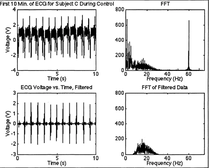
Instantaneous heart rate (HR) was calculated from the ECG data via peak detection using a matched filter. Appendix D contains the MATLAB© computer code used to do this. Since the subjects did not produce extremely high heart rates, it was acceptable to reduce the sampling rate of the data by 50%. The ECG data displayed typical baseline drift characteristics (low frequency noise) and in some cases extreme high frequency noise. The high frequency noise was a consequence not only of 60 Hz noise due to standard AC power supply voltage but also of AGS and subject movement. As a result, it was necessary to filter the signals. To see what frequency range the data were in, a 4096-point fast Fourier transform (FFT) of the first 10 s of data for each trial was performed. Figure 10 displays an example of the first 10 s of ECG data and its corresponding FFT. Note the large spike at 60 Hz due to standard AC power supply voltage. This spike was present in all of the ECG data. Also note the very strong frequency component near 1 Hz. This is most likely the baseline drift mentioned earlier. Since this experiment was interested only in heart rate, i.e. finding the QRS complexes, it was possible to use a very dramatic filter to eliminate as much noise as possible. The downside of the filter was to nearly eliminate recovery of P and T waves. A MATLAB© bandpass filter ("firl") of order 100 with cutoff frequencies of 10 and 30 Hz was used to "clean up" the ECG signal. The narrow frequency range of the filter was necessary to eliminate as much noise as possible (low frequency drift and high frequency noise) while still maintaining recovery of the QRS complexes after filtering. The

(33)

complex, hence the term matched filter. The MATLAB© function "fftfilt" was utilized to filter the ECG data. For our example in Figure 10, we see that the filtered data contains very little noise. One can actually detect P and T waves in this case. The FFT of the filtered data is also presented in Figure 10. Power at the main noise frequencies has been eliminated.

First 10 Min. of ECG for Subject C During Control FFT

4 800 2 600 0400 0 -2 200 -41 0 -M60 0 5 10 0 20 40 60 Time (s) Frequency (Hz)

ECG Voltage vs. Time, Filtered FFT of Filtered Data

3 800 2 600 >1 200 -2 -3 0 -0 5 10 0 20 40 60 Time (s) Frequency (Hz)

Figure 10. Example of Filtering of ECG Signals

The top left picture shows 10 s of the original ECG signal. The top right picture displays the FFT of the original signal. Note the large spike at 60 Hz. The bottom left picture shows the filtered version of the same 10 s of ECG signal. Note that P and T waves can be seen. The bottom right picture displays the FFT of the filtered data.

Peak detection was performed by looking for local maximums over time. Because noise could still be present in the filtered data, it was necessary to define a range of possible heart rates. The range used was 40-133 bpm. While transient, extreme increases in heart rate were lost, all of the averaged HR data points were well within this range. The times between successive peaks, R-R intervals, were found by simple subtraction of the peak times. Instantaneous HR-R was then

(34)

0.4 _{calculated by inverting the R-R intervals.}

0.3. At this stage some noise still remained. In

some cases the level of remaining noise

0.2.

was enough to severely alter the average

0.1 . heart rate, in most cases causing an

elevation. Generally, the noise data points were distinguishable from the real data by

-.1. having exceptionally high or low R-R

-0.2- .intervals compared to the main portion of

the data. Steps were taken to remove the

.30 10 20 30 40 so 60 70 so so T00 remaining noise data by setting bounds on

Figure 11. Impulse Response of the ECG Filter the R-R intervals. The bounds were set individually for each ECG signal and sometimes varied over the signal. The bounds used for each signal are shown in the MATLAB© codes entitled "heart*.m" in Appendix D, where * represents the individual subject code letter. Using the bounded instantaneous HR data, the average HR over 30 s and 5 min. intervals was found. Statistical analysis of HR utilized the values averaged over 5 min. HR comparisons between trials were based on differences while within-trial comparisons looked at the actual values. Since no evidence attests that heart rate will change proportionally under the conditions of the experiment, the HR averaged over 5 min. was normalized based on differences (similar to the BP normalization). The values at t = 25 min. were assumed to represent resting states. The mean resting values for the subjects (the average of the resting values from the four trails) were averaged, resulting in a group mean of 73.4 bpm. This group mean resting value became the value at rest (t = 25 min.) for the normalized HR data for each of the subjects. (Since the normalization was based on differences, no information was lost by using the group mean for the individual normalized values at t = 25 min.) The normalized HR at other times for the subjects was then calculated by adding to 73.4 bpm the difference between the actual HR at that time and the subject's actual HR at t =25 min.

Additional Procedures

Data were statistically analyzed using Student's t-tests for matched pairs. Unless otherwise stated, the n for all comparisons was 8. The primary comparisons explored were between the following pairs of time intervals: the first half hour of rotation in the G trials and the second half hour of supine rest in the control trial (comparison I), the first half hour of rotation in the G trials and the half hour of standing in the control (comparison II), and the one-hour rotation periods at