Efficient multi-bounce lightmap creation using GPU forward mapping

(1)

Efficient Multi-Bounce Lightmap Creation Using

GPU Forward Mapping

Doctoral Dissertation submitted to the

Faculty of Informatics of the Università della Svizzera Italiana in partial fulfillment of the requirements for the degree of

Doctor of Philosophy

presented by

Randolf Schärfig

under the supervision of

Prof. Kai Hormann

co-supervised by

Prof. Marc Stamminger

(2)

(3)

Dissertation Committee

Prof. Marc Langheinrich Università della Svizzera Italiana, Switzerland Prof. Evanthia Papadopoulou Università della Svizzera Italiana, Switzerland Prof. Marco Tarini Università degli Studi dell’Insubria, Varese, Italy Prof. Matthias Zwicker Universität Bern, Switzerland

Dissertation accepted on 18 October 2016

Prof. Kai Hormann Research Advisor

Università della Svizzera Italiana, Switzerland

Prof. Marc Stamminger Research Co-Advisor Universität Erlangen, Germany

Prof. Michael Bronstein PhD Program Director

(4)

I certify that except where due acknowledgement has been given, the work pre-sented in this thesis is that of the author alone; the work has not been submitted previ-ously, in whole or in part, to qualify for any other academic award; and the content of the thesis is the result of work which has been carried out since the official commence-ment date of the approved research program.

Randolf Schärfig

Lugano, 18 October 2016

(5)

Abstract

Computer graphics can nowadays produce images in realtime that are hard to distin-guish from photos of a real scene. One of the most important aspects to achieve this is the interaction of light with materials in the virtual scene. The lighting computation can be separated in two different parts. The first part is concerned with the direct illu-mination that is applied to all surfaces lit by a light source; algorithms related to this have been greatly improved over the last decades and together with the improvements of the graphics hardware can now produce realistic effects. The second aspect is about the indirect illumination which describes the multiple reflections of light from each sur-face. In reality, light that hits a surface is never fully absorbed, but instead reflected back into the scene. And even this reflected light is then reflected again and again until its energy is depleted. These multiple reflections make indirect illumination very com-putationally expensive. The first problem regarding indirect illumination is therefore, how it can be simplified to compute it faster.

Another question concerning indirect illumination is, where to compute it. It can either be computed in the fixed image that is created when rendering the scene or it can be stored in a light map. The drawback of the first approach is, that the results need to be recomputed for every frame in which the camera changed. The second approach, on the other hand, is already used for a long time. Once a static scene has been set up, the lighting situation is computed regardless of the time it takes and the result is then stored into a light map. This is a texture atlas for the scene in which each surface point in the virtual scene has exactly one surface point in the 2D texture atlas. When displaying the scene with this approach, the indirect illumination does not need to be recomputed, but is simply sampled from the light map.

The main contribution of this thesis is the development of a technique that computes the indirect illumination solution for a scene at interactive rates and stores the result into a light atlas for visualizing it. To achieve this, we overcome two main obstacles.

First, we need to be able to quickly project data from any given camera configuration into the parts of the texture that are currently used for visualizing the 3D scene. Since our approach for computing and storing indirect illumination requires a huge amount of these projections, it needs to be as fast as possible. Therefore, we introduce a technique that does this projection entirely on the graphics card with a single draw call.

Second, the reflections of light into the scene need to be computed quickly.

(6)

iv

fore, we separate the computation into two steps, one that quickly approximates the spreading of the light into the scene and a second one that computes the visually smooth final result using the aforementioned projection technique.

The final technique computes the indirect illumination at interactive rates even for big scenes. It is furthermore very flexible to let the user choose between high quality results or fast computations. This allows the method to be used for quickly editing the lighting situation with high speed previews and then computing the final result in perfect quality at still interactive rates.

The technique introduced for projecting data into the texture atlas is in itself highly flexible and also allows for fast painting onto objects and projecting data onto it, con-sidering all perspective distortions and self-occlusions.

(7)

Acknowledgements

First and foremost, I would like thank my advisor Prof. Kai Hormann for his support and guidance through the PhD-process. I am very grateful for his advice, his constructive criticism, and his encouragement and sincerity.

Furthermore, I would like to thank my external advisor Prof. Marc Stamminger from the University of Erlangen for his suggestions, insights and comments about my research.

I would also like to thank my internal committee members Prof. Evanthia Pa-padopoulou and Prof. Marc Langheinrich as well as my external committee members Prof. Marco Tarini and Prof. Matthias Zwicker for reading and evaluating this thesis.

I am also grateful to my colleagues here at USI with whom I had a great working relationship and many interesting talks. Especially Sandeep Kumar Dey and Dmitry Anisimov became very close friends during the time I spent here and helped me a lot in different situations. You guys made my life here very enjoyable even in days and weeks of extreme stress. I would also like to mention Ämin and Ali for the interesting talks we had about different topics.

Most certainly, I am indebted to my family, who laid the foundation for all I have and will accomplish in my life.

And most importantly, thank you Lilla for being part of my life and making me enjoy every minute of it to the fullest. You always gave me strength to work hard on this and lifted my spirit with your positive attitude towards everything. You managed to motivate me even during the hardest times.

(8)

(9)

Figures

1.1 Current computer graphics . . . 2

2.1 Lightspectrum . . . 8

2.2 Direct vs. indirect illumination . . . 11

2.3 Incoming light angle . . . 12

2.4 Material roughness . . . 13

2.5 Light reflection . . . 13

2.6 Phong-Shading-Components . . . 14

3.1 Raytracing vs. rasterization . . . 30

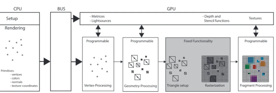
3.2 Fixed function pipeline . . . 33

3.3 Hardware Design . . . 34

3.4 Programmable pipeline . . . 35

3.5 OpenGL and DirectX timeline . . . 37

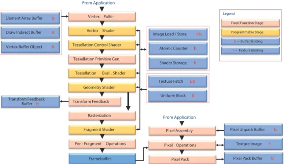
3.6 OpenGL-Pipeline . . . 38

3.7 Texturing example . . . 40

3.8 Lightmap example . . . 41

3.9 Texture composition example . . . 42

3.10 Mip-mapping and linear filtering . . . 43

3.11 Perspective effects on textures . . . 43

4.1 Projection goal . . . 48

4.2 Forward-Mapping . . . 49

4.3 Projection example . . . 51

4.4 Seam example . . . 53

4.5 Projecting over seams . . . 54

4.6 No texture coordinate sampling . . . 55

4.7 Subdivision scheme . . . 55

4.8 Tessellation example . . . 56

5.1 Mesh painting process . . . 61

5.2 Resulting texture atlas . . . 61

(14)

xii Figures

5.3 Brush examples . . . 62

5.4 Overview of the mesh painting algorithm . . . 66

5.5 Importance of VTC-precision . . . 67

5.6 VTC computation . . . 68

5.7 Painted mesh example . . . 70

5.8 Texture atlas for the mesh in Figure 5.7 . . . 70

6.1 VPL and sample visualization . . . 75

6.2 Visualization of light distribution on VPLs . . . 77

6.3 Radiosity projection process . . . 79

6.4 Seam repair process . . . 80

6.5 Problem cases . . . 81

6.6 Tessellation quality comparrison . . . 83

6.7 Improvement through soft shadows . . . 83

6.8 Importance of per-pixel shadow computation . . . 84

6.9 Detailed shadow example . . . 84

6.10 Different number of light bounces . . . 86

6.11 Example of slight scene changes . . . 86

6.12 Quality comparison with LuxRender . . . 87

6.13 Light distribution for the Cornell box with different numbers of VPLs . . 88

6.14 Comparison with texturing applied . . . 88

6.15 Correctness comparison with LuxRender . . . 88

6.16 Indirect illumination examples . . . 89

6.17 Requirements for smooth results . . . 91

6.18 Recomputation configuration . . . 92

6.19 Light recomputation configuration . . . 93

6.20 Single light changed . . . 94 6.21 Area light effect, created with our technique using 100 VPLs in 0.6 seconds 96

(15)

Tables

6.1 Timings . . . 90 6.2 Timings for recomputation . . . 94

(16)

(17)

Chapter 1

Introduction

Computer generated images for movies are nowadays often indistinguishable from real footage. Since there is no time limit for the computation of these scenes, everything is computed with very high precision to model reality as best as possible. Here the main focus is on following light rays or photons into the scene, which makes these techniques slow and computationally expensive.

But also interactive computer graphics has advanced to the point where it is possible to render scenes, objects, plants and characters in a way that makes the result hard to distinguish from a photography. All of the effects necessary to produce these results – e.g. dynamic lighting, subsurface and atmospheric scattering, depth of field, lens flares, high dynamic range lighting and more – are computed in real-time and react to current lighting conditions, material properties and other dynamic effects. Even dynamic reflections on arbitrary rough surfaces can be handled convincingly. Figure 1.1 shows examples from current computer games, rendered in realtime using the above-mentioned effects.

The techniques used in modern computer games include high detail textures giving materials a very natural look, tone mapping that helps to make the colors and con-trast more realistic, and image space reflections. Shaders allow each material to have entirely different visual appearance and can be used to approximate physical effects like subsurface scattering, diffuse and specular lighting effects for different BRDFs and so on. Normal mapping makes low-tessellated surfaces look like they have different roughness or impurities on them. Due to some simplifications of the physically-based formulas and the enormous parallel computational power of GPUs all of this can be handled in realtime and yet it gives incredibly realistic results as Figure 1.1 demon-strates.

As long as the virtual scene is rendered in the same style making every piece fit into the whole image, the user is inclined to take it for real. This is an important factor that makes it different to CG-effects in movies, where the rendered object needs to fit into the environment captured by the camera, because otherwise the viewer would immediately

(18)

2

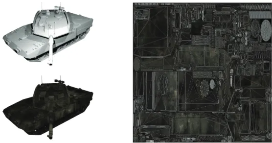
Figure 1.1. The left image shows a realistic looking scene with atmospheric light scatter-ing from the game Crysis 3 rendered in realtime. The middle image shows screen-space reflections, while the last image shows a scene from Call of Duty: Advanced Warfare, demonstrating the realism of scanned human actors rendered in realtime with depth

of field.

and intuitively spot the rendered objects which would destroy the immersion that a movie is aiming at.

Although all the above-mentioned techniques have been optimized for high speed computation as well as best possible looks, indirect illumination is still in a very simplis-tic state. In most cases it is modelled by artists or precomputed and the result is then used in the dynamic rendering process. This holds even for the Unreal Development Kit[16], which is considered the most advanced engine currently available. Although that gives good results, it restricts the rendering to rather static lighting conditions, while dynamic lights do not affect the scene ambience. Other approaches simplify the computation, allowing it to be computed at interactive rates, but the light distribution is very restricted. This approach becomes more and more popular recently and gives good results in generating a certain ambient, but since it is strictly bound in the num-ber of possible light bounces, it does not correctly illuminate scenes with complicated structures lit by only a few light sources. So if the user, for example, opens a door sep-arating a brightly lit room from a completely dark corridor, the direct light – if any is directed towards the door – would shine into the corridor and the door frames would create shadows. But the surrounding of the door would still stay entirely dark. The effect is even worse when the light inside the room is not directed towards the door. Then the corridor would stay entirely unchanged no matter if the door is opened or closed.

Therefore we propose a novel idea for computing indirect illumination that can be computed very fast and provides very convincing results. It uses a forward mapping approach that we introduce to create a smooth high-resolution light atlas for the scene. The light atlas allows us to use this results as long as the lighting computation in the scene does not change, resulting in very high rendering times. It allows for a fast recomputation of the lighting in case of only a few lights moving inside the scene.

Our proposed technique aims mainly at static scenes with mostly static light sources, yet allowing for moving objects and light sources, too. The technique is also highly scalable allowing to replace the real-time computation of the results by a more time consuming computation and therefore more precise result.

(19)

3 1.1 Research questions

1.1 Research questions

The main goal of this thesis is to create an algorithm that can quickly and precisely compute the indirect illumination solution for a scene and store the results smoothly and visually appealing. To achieve this goal, we have to answer two main questions first:

RQ1: How can indirect illumination be computed efficiently and flexible on the GPU? RQ2: How can the computation be simplified and speeded up without loss of physical

correctness?

There exist many techniques for handling these questions. Most of them fall into the categories of being either very fast and improving the overall visual quality of the computed scene but being not even close to the correct solution, while other methods compute the full physically-based solution at the cost of hours of computation time. Now we need to answer the question:

RQ3: How can the data be stored efficiently for visualizing the scene of interest? To answer this question, I decided to store the lighting solution within the texture atlas of the scene for which we compute the indirect illumination. This lightmap ap-proach is already very established, but here we present a physically correct and fast method to create it. To that end we need to figure out:

RQ4: How to efficiently project data from the scene into its texture atlas?

While texturing is standard nowadays for all kinds of graphical applications, the mapping of the object into the texture atlas is usually computed once and the texture is created accordingly. When projecting data from an arbitrary view onto an object, it will most likely overlap multiple seams. A seam is created by a mesh that is continuous in 3D, but separated into multiple patches within the texture atlas. That gives rise to the question:

RQ5: How can we project contiguously from a continuous mesh surface into the differ-ent related parts of the texture atlas?

When all the above questions are answered we need to ask the final questions: RQ6: How to compute the illumination and then project the result into the texture

atlas?

(20)

4 1.2 Contributions

1.2 Contributions

We present a novel technique that creates visually appealing indirect illumination, which is flexible enough to switch between high quality results that take a couple of seconds to compute but can be compared with state-of-the-art results and very fast pre-views that can be computed in almost realtime. Despite the very low quality of these previews, they still give a very good approximation of the overall lighting condition within a scene, thus providing artists with fast feedback during the light editing phase. The contributions in more detail are:

• We present an approach to project data from the surface of a given scene into its texture atlas. The technique is very flexible and can be adapted and opti-mized towards different goals. It is easy to implement into an existing render-ing engine and takes full advantage of the GPU’s extreme parallel computational power, making it extremely fast. In contrast to most other techniques, our so-lution is not fragment-bound and works efficiently for multiple high-resoso-lution texture atlases.

• To implement the projection technique, the main obstacle to overcome is the presence of seams on the 3D-mesh and to correctly project the data over them. In this thesis we present three approaches to handle that without much overhead in both memory and computational time.

• We present a technique for painting onto a 3D-mesh as a proof of concept of the above mentioned projection technique.

• Using the above technique in combination with a many-light approach we present a method that can efficiently compute and store indirect illumination for a given scene at interactive rates. It is almost entirely implemented on the GPU to guar-antee the short computational time and computes enough light bounces to come very close to the real solution for that scene.

• The method can also quickly recompute the entire solution for a scene in case a single light changes. Since our technique is deterministic in contrast to stochasti-cal methods like photonmapping, we can simply undo the effect of a single light and then recompute it with its new configuration. This restricts the computa-tion to only those parts of the scene, where the change in the lighting situacomputa-tion actually takes effect.

• The technique is very flexible and can compute physically realistic images with smooth shadows in seconds as well as previews in realtime. While these previews have harder shadows and do not look as visually appealing as the results created by the longer processing, the physical correctness is preserved. This makes the preview optimal for editing the lighting situation in virtual scenes.

(21)

5 1.3 Outline of the thesis

1.3 Outline of the thesis

We start by giving an overview of the general physics of light in Chapter 2. This chapter also descibes the difference between the computation of direct and indirect illumination in virtual scenes. We end that chapter with an overview of the state of the art in indirect illumination computation.

We begin Chapter 3 by describing the history of the graphics hardware as well as the APIs that allow for programming them. Based on that we show how this led to different techniques that allow drawing onto or projecting data into the texture atlas of a virtual object and how these techniques became much more effective with the advancements in the underlying hardware.

In Chapter 4 we describe the idea of forward mapping that allows us to project data from screen space into the parts of an objects texture atlas visible on the screen. This mapping is not fragment-bound since it draws only into the necessary parts of the – possibly many different – texture atlases. This allows for fast computation of results even for multiple high-resolution texture atlases.

In Chapter 5 we present an application that uses forward mapping to allow artists to view a scene or an object on screen and then paint directly into the texture atlases of this object or scene.

In Chapter 6 we introduce a new approach to compute indirect illumination within a scene that strongly depends on the forward mapping to create and store the final results. We explain our multi-light approach for distributing the light and how we adapted the forward-mapping approach to suit the needs of this application.

We conclude the thesis with Chapter 7 by putting the current work into the context of the field and by describing how the research questions are answered to achieve the presented work. We furthermore give an outlook on how the work can be improved and optimized further.

1.4 Publications

The work presented here led to two publications. The first paper is a proof of concept for the efficiency of the forward mapping approach, using mesh painting as a demonstra-tion. The second paper describes our approach to the problem of efficiently computing and storing indirect illumination results.

• Chapter 5 is based on the forward mapping technique that was presented at the VMV 2010 conference and published in the proceedings Vision, Modeling & Visu-alization[47] with the title “Hardware Accelerated 3D Mesh Painting”.

• Chapter 6 is based on the work that was published in the journal Computers and Graphics [48] with the title “Creating Light Atlases with Multi-bounce Indirect Illumination”.

(22)

(23)

Chapter 2

Basics of Light and Lighting

In this chapter we give an overview of the physics of light and its interaction with objects in Section 2.1 and the perception of light and color in Section 2.2. With these basics we then describe to mathematical descriptions that capture this light interaction and can be used to model lighting in virtual scenes in Section 2.3.

In Section 2.4 we describe different models for direct lighting and then go into de-tails about indirect illumination and why these two models need to be separated in Section 2.5. In Section 2.6 we describe the current state of the art in computing global lighting conditions with close to realtime frame rates and also describe techniques aim-ing for perfect results, where the computational time is irrelevant.

2.1 Physical properties of light

Let us start by describing how light interacts with surfaces and capturing devices as well as the human eye. The lighting condition in an arbitrary surrounding is given by the photons that are created and emitted from any direct light source and are then reflected and refracted from any surface – and partially even by atmospheric effects like fog – in the scene. What we perceive visually is the combination of all of these interactions with the photons that end up in our eye.

With our eyes or any capturing device like e.g. a camera we see the world as a sum of the photons, that are ultimately reflected into the visual sensor. There the final image is created as a measurement of the number of photons giving the brightness in every perceived point and the wavelength giving the color of that point.

The interaction of the photons with the sensor are described in Section 2.2. The brightness of a point on an object or light source is given by the number of photons that arrive at the sensor from this given point (for more details see Section 2.2.1) and is measured in Lumen[Lm].

The color of an object is given by the wavelength of the photons being reflected by this objects surface properties. Each photon is an electro-magnetic wave with

(24)

8 2.2 Perception of light

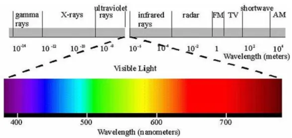
Figure 2.1. The lightspectrum going from blue on the left side (short wavelength) to red on the right side (long wavelength). Note that the visible part is just a small fraction of the continuous electro-magnetic spectrum.1

ticle properties moving with the speed of light c in a certain direction with a given wavelengthλ related to the photon’s energy E through E =hc_λ, where h is the Planck constant. The photon’s wavelength is what we perceive as color. The continuous color-spectrum is depicted in Figure 2.1.

The surface of an object might reflect photons with one wavelength while absorbing photons with another one. The wavelength of the photons that get reflected, determine the color of the object (more details about that can be found in Section 2.2 and the mathematical model that describes the light interaction in Section 2.3).

In the absence of extraordinary strong gravitational forces, a photon will travel on a ray from its point of origin, until it interacts with the surface of an object, at which point the direction will change – that is, if the photon does not get absorbed – and it will travel along the new ray.

2.2 Perception of light

Human eyes perceive light in two different ways. In dark environments the eyes rely on the rod cells, that react to light around 500 nm wavelength (blue-green). Since all rod cells react to this same wavelength, they do not allow us to differentiate colors, but due to the high concentration of Rhodopsin, they enable us to see in dark environments, since they are around 1000 times more sensitive than the cone cells, that allow us to perceive colors.

(25)

9 2.2 Perception of light

For bright environments the eye possesses three different types of cone cells, one type for each of the colors red (500-700 nm), green(450-630 nm) and blue (400-500 nm). They use slightly different variations of the molecule Photopsin, that reacts to different wavelengths. Incoming photons of a certain wavelength therefore create a re-action in the corresponding cells. The signal created by the three cone cells is then com-bined by other cells through the step-wise adaptive blending r+ g + ((r + b) + (g + b)) into a single color signal that is send to the brain together with a signal encoding the overall brightness.

In monitors the same composition method is used to create the different colors on displays. Each pixel has a mask for the three colors red, green and blue which are used to dim the corresponding portion of the white background illumination. Each mask is controlled by a byte that sets the amount of light that can pass through that color-channel with 1 meaning all light can pass and 0 that meaning the mask absorbs all the amount of the specific color. This way we end up having a 24-bit color range, leading to 224= 16777216 different colors (Note that it also contains the same color in different brightness shades).

Since the number of photons define the brightness, the mask does not only control the color itself, but also the brightness that is perceived, ranging from the brightness of the background illumination to the amount that can still pass through the color-mask set to full absorption. In the optimal case this would be completely black, meaning no photons passed, but due to technical restrictions this value will be higher than that.

2.2.1 High-Dynamic-Range

As mentioned before, the brightness is measured in Lumen, where 1 Lm at a wavelength of 555 nm is equivalent to a photon rate of 4.11× 1015photons per second.

Each photon creates a single chemical reaction, triggering a signal to the brain, and the signal strength is given by the amount of reactions within a given time. Let aside the color-perception described in Section 2.2 and looking at just one arbitrary receptor-cell, the brightness that can be perceived is given by the maximum number of signals that the cell can create in a given time-interval for a single measurement.

Since the brightness varies strongly between bright daylight and a night with noth-ing but starlight, the human eye adapts to the current brightness level through changes in the pupil dilation – adapting the number of photons entering the eye – and by chang-ing the sensitivity of the photo-receptor-cells – changchang-ing the signal strength from the retina to the brain.

Since the human eye is additionally made up of rod and cone cells that operate at different brightness-levels, the overall visual range is further increased. This extreme range is called High-Dynamic-Range(HDR) in computer graphics due to the strong con-trast of the brightness range of the monitor (1:1000) which is now usually labelled as being Low-Dynamic-Range.

(26)

10 2.3 Lighting in virtual environments

Currently the problem is solved by compressing the brightness range of images with a tone mapping. This technique applies non-linear curves on the input colors to compute output colors that match the contrast and luminosity as best as possible over the whole image.

With HDR-monitors becoming widely available, the correct computation of indirect lighting that illuminates every part of the environment – and be the quantity ever so small – becomes more and more important. In contrast to the Low-Dynamic-Range screens, where an approximation of the brightness is enough to give a feeling of realism, since the image is compressed to 8 bit per color channel with tone-mapping, with HDR-screens the brightness needs to be computed with high fidelity to achieve the sense of looking at a realistic scene.

2.3 Lighting in virtual environments

In computer graphics we deal with virtual scenes or objects mainly given as triangular meshes. Other representations like point-clouds and implicit functions describing the surface have also been experimented with, but triangle meshes proofed to be the most efficient (see Chapter 3). To give these scenes and objects a natural look when being rendered, they need to be correctly lit, since their interaction with light is what we perceive (see Section 2.2).

To achieve this, we need to understand the physical basis of lighting to compute these effects in the virtual environments.

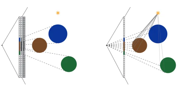
As mentioned before, the brightness is given by the number of photons. These photons originate from a light source (direct light), but might also have bounced off of surfaces in the scene (indirect illumination, more about this in Section 2.5). Figure 2.2 shows a comparison. The further away we get from any light source (direct or indirect), the fewer photons we register on the same area. This number falls off with a factor of

1

r2, where r is the distance to the object, since the photons are distributed on the surface

of the sphere with the radius r, which grows by r2.

Now that we have covered the basics of the light origin, we need to look at the interaction of the photons with objects. Note that the following three types of inter-actions describe what can happen to a single photon. In reality one surface can – and most likely will – show different types of interaction. That is, each photon interacts in a single random way with the surface, but the probability of the exact interaction of the photon is given per every material. Furthermore, these probability distribution differs for every wavelength, leading to this materials reflection coefficientsρ, that describe the probability distribution for each color:

• Absorption: its energy is transformed into heat and no further interactions can occur with this photon.

• Translucency: the photon passes right through the object, changing its trajectory due to the refraction index of the material.

(27)

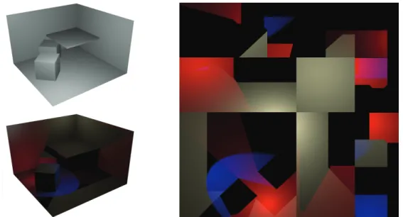
Figure 2.2. Difference between direct light (left) and indirect illumination (middle). The final solution is composed of both parts (right).2

• Reflections: Materials reflect light in different directions with different inten-sities due to microscopic inter-reflections on rough surfaces and other effects. Each single reflection follows the law of reflection (specular), but for rough or weakly translucent surfaces a number of inter-reflections occur leading to diffuse reflections or subsurface scattering respectively.

– Specular: the photon is reflected along the reflection vector. Details about this can be found in Section 2.3.2.

– Diffuse: the photon is reflected into a random direction away from the surface. Details about this are described in Section 2.3.1.

– Subsurface-Scattering: the photon enters the material and gets reflected many times before leaving the surface in a random direction close to the entry point.

The interactions that make up most parts for most materials are the diffuse and specular reflection as well as the absorption of the incoming light. Therefore we look into this more closely now. We will start with the diffusion term in Section 2.3.1 and then look into the specular reflection in Section 2.3.2.

2.3.1 Diffuse reflection

The diffuse reflection is created by light being reflected in the top layer of a surface one or more times. Due to the possibly high amount of inter-reflections, the reflected light can be assumed to be reflected equally in all directions away from the surface, although the exact BRDF might be slightly different. To determine the brightness of a fully diffuse surface it is therefore enough to compute the incoming radiosity, since the reflected light is in all directions a certain fraction of this value.

We describe the diffusion term now by looking at an exemplary interaction of light with a plane surface. First we look at a light ray R with a certain width w. The amount nof photons in the cross-sectional area of this ray is given by the brightness of the light source from which it originates (see Figure 2.3). For simplicity we ignore the reflection

2_Image _taken _from: _{https://docs.unrealengine.com/latest/INT/Engine/Rendering/}

(28)

coefficient of the plane material for now and assume that all photons are reflected diffuse (ρ_s= 0 and ρ_d= 1). The perceived brightness of a surface area A is then given as a fraction of the amount of photons that impact in A.

width N N α width α . A

Figure 2.3. When the light shines perpendicular onto a surface, the lit area has the same size of the incident light ray (left). If the light hits the surface with an angleα

bigger then zero, the lit area becomes bigger then the with of the light ray. Therefore the amount of light energy is distributed over a bigger area which makes each point within this area darker, the bigger the angleαgets.

If the light ray intersects the plane straight from the top, the illuminated area A has exactly the width w as seen on the left side of Figure 2.3. Therefore all n photons contained in the cross-section of R impact the area A. If the incident angleα between the normal N and the light ray R is bigger then 0°, the area will be bigger then w. Using trigonometry (image on the right side of Figure 2.3), we see that we have a 90° triangle given by the light ray R. Since the sum of all angles in a triangle sum up to 180° and we have a 90° angle between R and w, we know thatα + β = 90°. The angle α occurs also in the triangle where w is adjacent toα.

The lit area A0is now given as _cosw_(α) since it is the hypotenuse of the triangle with wadjacent to it. Let the number of photons in the cross-section of R be n which leads to a photon density of _wn. With R having an angle of α with the normal, the photon density now becomes nw

cos(α) = n cos(α)

1

w. Since the width is infinitesimally small and

the number n of photons is set for the light source, we see that the amount of photons hitting the surface can be computed by multiplying the brightness of the light source with the cosine of the angle between the normal N of the surface and the light-ray R.

2.3.2 Specular reflection

Perfect specular reflection describes the effect that is given by a mirror. A light ray R hits a surface with a certain incoming angleγ measured between R and the surface normal N and are reflected of the surface in the direction with the same angle to the normal

(29)

in the other direction within the plane created by the vectors R and N (see Figure 2.5 left).

The explanation for that is the electro-magnetic-wave-character of light. When the light wave hits the object, the Huygens-principal creates a wave-front with the same angle to the surface, as the incoming angle but in the opposite direction.

Figure 2.4. Here different values for the roughness of a material are shown. With grow-ing roughness, the reflection coefficients change from high specular and low diffuse to low specular and high diffuse (from left to right).3

The reflection vector can be computed as R0= 2〈N, R〉N − R. An approximation for that is to use the half-vector as suggested by Blinn[3]; it uses the fact, that _||R||R +_||RR0₀_|| will create a vector that is completely aligned with N . If the vector C from the point to the camera is equal to R0, the reflection is perfect and the camera will receive the full reflected intensity. If the vector from the point to the camera deviates, the intensity should decrease. It can be computed as_{〈N , (R + C)〉}ρs4 _{as the brightness given by the}

specular reflection. This is 1 for C= R0, while the value quickly decreases the further C deviates from R0. Computing this is faster and gives results very close to using the ones computed with the true reflection vector. Figure 2.4 shows examples of different values for the specularity of an object.

N

α α

Figure 2.5. The incident angle is equal to the reflected angle for ideal specular reflec-tion (left). For different materials the light flux is highest around the reflecreflec-tion vector and falls off quickly with increasing divergence from it (lenght of blue arrows on the right).

3_Image _taken _from: _{https://docs.unrealengine.com/latest/INT/Engine/Rendering/}

(30)

14 2.4 Direct illumination

2.4 Direct illumination

For efficient rendering we differentiate between direct lighting and indirect illumina-tion (see Secillumina-tion 2.5) which is visualized in Figure 2.2. Direct lighting – also refereed to as local illumination – describes the effects created by light being emitted from a direct light source, hitting at most one surface and then being reflected directly into the cam-era where they contribute to the color and intensity of a single pixel. In the beginning of computer graphics, objects were not illuminated at all and were simply assigned a fixed color. Then simplified lighting models were created, that approximated realistic light-ing effects fast enough to be computed. The first of these techniques was flat-shadlight-ing, where the color of a triangle was determined by the cosine of the angle between its normal and the light-ray. In 1971 Henri Gouraud[18] improved this by computing the lighting at every vertex of the triangle and interpolate the resulting colors over the tri-angles surface. Since this still created artefact when dealing with specular reflections, Bui Tuong Phong[41] proposed in 1975 to interpolate the normals across the triangles surface and then compute the lighting per visible pixel with this normals.

These and other techniques are based on the Phong lighting model[41], that takes into account the self-emitted light of an object, approximates the indirect illumination by a simple constant color (omnidirectional) and then sums up the effects of all direct lights in the scene. This is done by splitting them into a diffuse and a specular com-ponent. It furthermore takes the materials reflection coefficients into account, which describe how much of the incoming light is absorbed. The whole computation as well as the reflection coefficients are usually given in the RGB-color-space (see Section 2.2).

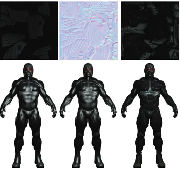
Figure 2.6. The different components for Phong-shaded objects. In this shading, the global lighting situation is simplified to be a constant color.4

Since all lighting computations are based on this equation we describe it in detail here: R= E + ρ_aA+ L X i=0 I_i(ρ_dD_i+ ρ_sS_i)V (i) (2.1)

4_Image _taken _from: _{https://en.wikipedia.org/wiki/Phong_shading/media/File:Phong_}

(31)

15 2.5 Indirect illumination

where R is the color of the current pixel, given as the sum of the self-emitted light E, the overall ambient color A and the sum over all L light sources with intensities I_i interacting with this point. The interaction between the light and the surface itself is separated into a diffuse interaction D_idescribing the reflection of the light equally in all directions (see Section 2.3.1) and a specular term S_i that describes the light reflection according to the law of reflection (see Section 2.3.2).

The amount of light reflected from the surface point is a property of the material at that position and given by the reflection coefficientsρ which are material parameters given in the RGB-color-model describing which light waves are absorbed and which get reflected. The parameters are usually given for ambientρ_a and diffuseρ_d reflections. The specular reflection coefficientρ_sshould have the same values across the colors for dielectric materials since they reflect all wavelength equally, while they are material color dependent for other materials such as metals.

These terms are evaluated as

Di= 〈Li, N〉 (2.2)

where L_iis the normalized vector from the point of interaction to the light source i and N is the normalized normal at the point of interaction. The specular term is evaluated as

Si= (〈2〈Li, N〉N − Li, C〉)s (2.3)

with C being the vector from the point of intersection towards the camera. The ex-ponent s is a surface property describing the shininess of the surface. As mentioned in Section 2.3.2 this can be simplified by the use of the half vector leading to similar results. An example that separates the results of the different terms is visualized in Figure 2.6.

The function V(l, i) describes the visibility of point i from the light source l and de-termines if the point is shadowed (V(l, i) = 1) or lit (V (l, i) = 0). In modern interactive visualizers this is determined through shadow mapping, which is hardware accelerated on all modern 3D-accelerators. Another technique that was quite popular for a while was to use the stencil-test for shadow-volumes, but shadow mapping has proven to be superior and is nowadays the standard.

2.5 Indirect illumination

Indirect illumination in contrast to local lighting as described in Section 2.4 describes the illumination created by light that was reflected off of at least two surfaces. When light hits a surface, it can be refracted leaving the object at another point than where it entered the object. Another possibility is that the energy is absorbed by the material it hit; in this case the photon’s energy is transformed into heat. The third case is, that the light bounces off the surface either in a random direction (diffuse reflection) or it is reflected (specular).

(32)

In real world materials all of the above might happen at once. A good example for that are thin leafs on a tree. They let a fraction of the light through (refraction), absorb another part (heat and photo-synthesis) and reflect the rest both diffusely and specularly.

Even black materials reflect at least a small fraction of the incoming light which makes indirect illumination hard to handle. This is due to the fact, that light bounces off of every surface, and though the intensity might have been reduced by a huge amount due to the reflection-coefficient of the surface material, it will now serve as a weak light source itself, illuminating objects in its vicinity.

This effect occurs wherever light hits a surface, and every photon is reflected until it is absorbed. To compute the global lighting means therefore to follow all possible light paths ad infinitum in contrast to direct illumination, where we just compute the lighting situation for every visible point on the screen.

In Section 2.5.1 we describe the history and basic idea of global illumination, clas-sify different approaches to that problem in Section 2.6 and then describe state-of-the-art ideas in Section 2.7.

2.5.1 Basics for implementation

When the importance of indirect illumination in rendered scenes became obvious, the first approach of computing it was through the radiosity equation formulated by[5]. The authors’ radiosity method describes an energy equilibrium (see Eq. (2.6)) within a closed surface assuming that all emissions and reflections are ideal diffuse. The au-thors further partition the whole scene into a finite number of n small patches. These patches are associated with a position x_i– the center of patch i – and the normal of this point. With this assumption and simplification they reformulate the rendering equation introduced by[27] to the following:

B_i = E_i+ p_i n

X

j=0

B_jF_{i j} (2.4)

where B_i is the radiosity of the current patch i (the amount of light leaving), E_i is its self emission, p_i is the percentage of light that gets reflected from patch i and the sum over all the n patches that make up the environment takes into account the amount of light reaching the current patch through light that is reflected or emitted from other patches in the scene. Therefore B_jdescribes the amount of light that leaves the patch j and the form-factor F_{i j} describes the geometric relationship between the patches i and j and therefore the percentage of the light leaving patch j and reaching patch i. The F_{i j} for patches with areas A_i and A_j is defined as:

Fi j=

1 A_i

cosθ_icosθ_j

(33)

were the angles θ_i and θ_j in the cosine terms describe the angle between the direct line between the two patches i and j and the corresponding normal vector for these patches, and r is the distance between the patch i and patch j.

In case of partial occlusion between two patches the authors suggest to subdivide them to get a better result. The authors also mention that for a finite area the form-factor is equivalent to the fraction of a circle covered by the projection of the area first onto the hemisphere and then orthographically further down onto the circle that is the basis of this hemisphere. By subdividing the hemisphere into smaller patches itself and computing the projection of other patches on them and only considering the closest patch that gets projected to each element, it also takes care of occlusion. The solution found for these small partitions of the hemisphere – called delta form-factors by the authors – for one distant patch can then be summed up to get the form-factor between the current patch and this distant one.

With these form-factors and the initial emission values E = (E₁, . . . , E_n) for all patches the authors solve the following equation system to receive the final radiosity B= (B₁, . . . , B_n) for all the patches in the scene,

     1_{− p}₁F11 −p1F12 · · · −p1F1n −p2F21 1− p2F22 · · · −p2F2n .. . ... ... ... −pnFn1 −pnFn2 · · · 1 − pnFnn           B1 B2 .. . B_n      =      E1 E2 .. . E_n      (2.6)

The authors use scenes made up of polygons that are also used as the patches. After they have solved the linear equation system and get the radiosity of each patch, they render the scene using bilinear interpolation on the vertices to get a color out of the polygons/patches surrounding this vertex. This way the resulting image looks smooth, since there are no sudden jumps in color or brightness. We described this technique in much detail, since it introduces many tricks that are standard for computing radiosity nowadays.

The idea of solving the equation system to compute the final radiance for the scene is the basis for modern shooting or gathering techniques. These techniques take ad-vantage of the fact that in the first step of the algorithm only the light sources possess energy that needs to be projected into the scene, and even in the next few steps there are some elements that do not contribute to the light distribution because at this stage they still did not receive any light. The first approach to use this fact was only comput-ing the lines in the matrix that have a value greater then zero on the right side. Later, shooting and gathering approaches were introduced and even ported onto the graph-ics card, as described in the work of[7], for example. Their technique stores for all patches in the scene the energy that they distribute in a sorted list where elements with the highest energy come first. Then the elements shoot their energy into the scene in the given order and are set to have zero energy afterwards. This process permanently introduces new elements into the list and updates elements that are already stored,

(34)

18 2.6 Classification of indirect illumination techniques

since their energy level increases. This way the whole list is processed until the next element in the list has a radiosity that lies under a certain threshold, which terminates the computation, since the energy is distributed well enough.

Since the field of indirect illumination is large and diverse, we start this partitioning the field into smaller sub-fields (e.g. interactive vs. non-interactive) in Section 2.6. This is important, since the computational cost of indirect illumination is very high, and one needs to choose between perfect results and real-time computation. For light-editing a trade-off between these two might also be desirable. The comparison of existing techniques only makes sense within one of these classes. We then give an overview of the techniques that are state of the art in each field in Section 2.7, concentrating on the field of this work being close to real-time computation of the indirect illumination solution.

2.6 Classification of indirect illumination techniques

Since the beginning of indirect illumination computation, different approaches with deviating aims were developed for its computation, so we first distinguish between these varying techniques and create clusters. The first approaches date back into the 1970ies and since then one goal was to make the computation of indirect illumination ever more precise. As computers got faster and the results for diffuse surfaces led to good results, the focus shifted from making it more and more realistic to making indirect illumination computation also faster, since achieving interactive frame rates became a realistic goal. When the first 3D-accelerators were introduced in 1996 and newer versions supported hardware-accelerated Transforming & Lighting in 1999, researchers focused on this goal. The research was now focused on the different path of either increasing the realism of the results by taking into account more and more physical interactions of materials with light into account while others the quality and instead tried to compute visually appealing but not physically correct results in real-time.

If we take a look at the varying techniques that exist today it is convenient to sep-arate them into different classes. There are techniques that compute indirect illumina-tion almost in real-time – something around 30 frames per second (FPS). These ideas make strong simplifications or compute only one or two light bounces to achieve this. Within this class of techniques another criterion for further distinguishing is the num-ber of bounces the algorithms can compute. Another class of techniques do not aim for high framerates and instead aim at increasing the realism of the computed images. These techniques have to compute all light bounces – meaning they have to follow the light until its energy falls below a certain threshold.

To simplify the distinction, we concentrate on the class of real-time algorithms. Most compute only a single bounce of light and the reason for this is twofold: On the one hand, it might be sufficient in small and simple scenes to just compute one bounce while computing more would just be a waste of computing time. On the other

(35)

19 2.6 Classification of indirect illumination techniques

hand, it is much faster to compute only one inter-reflection, since this is the most time consuming part of indirect lighting computation after all (even if pre-computed light transport functions are available).

So for simplicity let’s say we have the following classes: • Interactive Frame Rates

– One bounce reflections – Multi bounce reflections • Non-Interactive Frame Rates

Now that we have partitioned the existing algorithms into these groups, we can also distinguish between the following main ideas of how to scatter the light:

• Computationally

– Discretizing the scene (Radiosity) – Many-light approaches

• Statistically – Ray-tracing – Photon-mapping

While the computational method via the form-factors is very time consuming, it is also very precise. It partitions the scene until the discrete parts (patches) are small enough to give good results. Modern methods also partition the scene depending on the al-ready computed results and their quality, to only improve the computed results where necessary, speeding up the computation time considerably. But still, doing the visibility test between each pair of surfaces is very expensive.

The other idea is to use the Graphics Processing Unit (GPU) to handle this visibility test via rendering the scene from the current light source’s point of view. This can be done very efficiently, because it uses the graphics card for its main purpose and the extreme parallelism is optimally used. But then other problems arise, like for example getting all necessary data for a distant surface that is interacting with the current one. One reason for this is that the graphics card does not allow random access to its memory. Another idea using the GPU is to create new light sources and use the shadow mapping algorithm implemented in modern graphics cards to do this computation as if it was done for a direct light source. This gives good results but is still quite expensive. While both techniques can be used for interactive computation, it is mainly the latter that is actually used nowadays.

The other two techniques – ray-tracing and photon-mapping – are mainly used for non-interactive computation of indirect lighting, since they are very precise but also

(36)

20 2.7 Overview of existing techniques

computationally expensive. Both methods do not calculate the lighting distribution based entirely on a physical model but instead use a stochastic approach for scattering light from every point that has gathered light in a previous step.

Another differentiation that is needed is concerned with the material properties that are supported. Most techniques do not allow for glossy materials, since the ap-pearance of the light also depends on the current viewing direction. Other techniques do compute one bounce (the last one of the indirect lighting computation) to consider glossy materials. But this almost only holds for interactive techniques, because the non-interactive techniques can easily take care of this, since the additional computational cost is irrelevant and negligible.

So if we want to distinguish the different techniques, the most realistic partitioning is:

• Interactive Frame Rates – One bounce reflections

glossy reflections diffuse materials only – Multi bounce reflections

glossy reflections diffuse materials only

• Non-Interactive Frame Rates (mainly Photon-mapping or ray-tracing) – multiple bounces

• Full Solution

– very many bounces

– complex material-light-interaction with diffuse and glossy reflections BRDF

subsurface scattering refraction

2.7 Overview of existing techniques

There are many techniques based on the before mentioned light distribution model. We will now give an overview of the state-of-the-art techniques. We start with the histor-ically first implementations and there direct improvements in Section 2.7.1. We then look at techniques that achieve interactive rates in Section 2.7.2 and finally describe methods that aim for photo-realistic results in Section 2.7.3.

(37)

2.7.1 Non-Interactive approaches

In this section we discuss techniques that improve the computational time by optimiz-ing other algorithms through parallelization and/or porting them to the GPU without achieving real-time-speeds.

The first approach of computing indirect illumination was through the radiosity equation formulated by Cohen and Greenberg[5]. This radiosity method describes an energy equilibrium within a closed scene assuming that all emissions and reflections are ideally diffuse and the light distribution is computed iteratively over the discretized surface of the scene.

Then shooting and gathering approaches were introduced and even ported on the graphics card by Coombe et al.[7]. This technique uses the aforementioned approach for the coarse distribution of light within the scene, followed by a highly precise method for storing the lighting results, therefore changing the geometry of the scene and cre-ating a higher tessellation. In our approach we only use the shooting method in the beginning of the light distribution and then switch to a scene texture atlas for storing the high resolution results. Therefore, our approach does neither depend on nor does it change the scene geometry. Szécsi et al.[55] propose to precompute the expensive integrals needed for indirect illumination for all but one variable, the light position, and store them in a texture atlas of the scene. During rendering, the radiance of the visi-ble scene pixels is determined by evaluating this precomputed data for the given light positions. Although the results look very promising, the amount of memory needed is rather big, even for scenes without complex occluder configurations. Our technique can handle complex scenes using only a light atlas, which is required anyway.

Arikan et al.[2] accelerate the final gather step of global illumination algorithms through approximation of the light transport by decomposing the radiance field near a surface into separate near- and far-fields which then get approximated differently. They rely mainly on the assumption that radiance will exhibit low spatial and angular variation due to distant objects, and that the visibility test between close surfaces can be reasonably predicted by simple location- and orientation-based heuristics. They use scattered-data interpolation with spherical harmonics to represent the spatial and angular variance for the far-field, while the near-field scheme employs an aggressively simple visibility heuristic.

Other techniques [20, 23] use the extreme parallel capability of modern GPUs to accelerate ray-tracing approaches. They cluster different light rays according to their direction and then use the GPU to compute the visibility for all these bundles simulta-neously. This makes the computation much faster than on the CPU, but still does not achieve interactive frame rates. Our technique creates similar quality, but in shorter time.

Luksch at al.[36] propose a technique for computing the light atlas of a scene at almost interactive speed. They partition the scene into polygons and distribute the light energy among virtual light sources, one for each polygon. In a final gathering

(38)

step, they render the light atlas and collect the radiosity for each texel from the direct and virtual light sources. Although this technique is similar to ours, it is limited to two light bounces and therefore produces results with a lower quality.

2.7.2 Interactive approaches

An important technique considering indirect illumination was introduced by Greger et al.[19]. Instead of calculating the indirect lighting situation within a given scene, it rather tries to compute the illumination introduced by the scene on a static object moving through the scene. That means that the scene lighting needs to be already computed, for example by the previously described radiosity method. Under the as-sumption that this is given, the idea behind irradiance volumes (IV) is that instead of storing the amount of light leaving each surface point within the scene, it rather pre-computes for certain points in space the incoming light under certain angles. To do this, the technique first fills the bounding box of the scene with virtual spheres – the irradiance volumes – that are distributed through the scene in a way that best sam-ples the underlying geometry and its complexity. Then each sphere samsam-ples the space around with a specific step size, resulting in the projection of the scene around the sphere on its surface with the pre-computed brightness and color. That means that every sphere is “lit” by its environment. The authors then store these color values for every sphere and use them for the objects moving within the scene. Therefore, a mov-ing object is first associated with the closest irradiance volumes and the object’s surface color is then computed by taking into account the object’s normals and the distance to the spheres using bilinear interpolation of the color values determined. This technique is only able to compute indirect lighting for moving objects within a scene for which the indirect illumination was already computed. This means that this technique cannot handle changes of light sources within the scene and is therefore bound to statically lit environment.

Sloan et al. [52] introduce a technique that extends the idea of IV through pre-computed radiance transfer (PRT). The authors describe a technique that can handle the different lighting effects introduced in[19], but also takes into account inter-object reflection and shadow casting. This is done by a pre-computed spherical harmonic ba-sis that describes how an object scatters light on itself and the surrounding space. Like in the previous idea of IV, the lighting environment is assumed to be given and being infinitely far away, which makes the illumination the computation of a cosine-weighted integral for each surface point of the object if it is convex. For concave objects the inte-gral is multiplied by a value that describes visibility along each direction to account for self-shadowing. The authors pre-compute these values and the integrals and represent it through spherical harmonics. Through the linearity of this representation the inte-gral of the light transport function becomes a dot product between the pre-computed environment light and the pre-computed coefficient vectors that can be handled by the graphics hardware in real-time. In the same way the technique also handles glossy

(39)

surfaces, inter-reflection, and soft-shadows.

Sloan et al.[53] extend the paper [52] to account for deformable objects in a local PRT considering the inter-surface reflections and shading of a surface point by nearby surroundings. This is done by switching from the pre-computed spherical harmonics basis to the zonal harmonics basis, which allows for fast computations of rotations. So whenever a part of the object is deformed, the local basis is updated to fit this deformation. Afterwards the transformed basis is used to compute the resulting lighting for this object.

Kristensen et al.[29] presented an algorithm that is able to indirectly relight scenes in real-time. This is achieved by extending the idea of precomputed radiance trans-fer and introducing the idea of unstructured light clouds to account for local lighting. The indirect illumination of a static scene is precomputed for a very dense light cloud, which is then compressed to contain just a small number of lights. While rendering the scene, its indirect illumination is approximated by interpolating the precomputed radiosity of the closest lights in the light cloud. This requires a relatively high number of values stored for every vertex of the scene and can only compute the lighting at these scene vertices. Therefore, the quality of the resulting image depends strongly on the tessellation of the scene. The technique gives nice results in static scenes with moving lights, but it cannot handle scene changes or large moving objects that strongly change the scene’s lighting situation. Instead, our technique uses a high resolution texture to store the indirect shadows, which allows us to handle even high frequency lighting details. Moreover, our technique does not require any further computations once the light distribution is stored, which in turn reduces the time needed for rendering every frame.

Another approach was introduced by Walter et al. [57]. The authors suggest an algorithm that can handle all kinds of light, e.g. environment maps and indirect il-lumination. The main idea is to simplify huge amounts of light sources by grouping them together and only to compute the illumination effects for the light sources cre-ated through this combination process. To speed up this merge and make it as accurate as possible, the authors introduce a binary light tree combined with a perceptual met-ric. While the former helps in finding appropriate light clusters, the latter helps to stop clustering if the introduced error exceeds a certain threshold. This way the rendering time can be reduced, while at the same time a certain quality for the final result can be guaranteed. For indirect lighting the authors simply use their algorithm – which they claim to be able to reduce hundreds of thousands virtual lights to only few hundred shadow rays – to reduce the expanse in computation. To calculate indirect illumination they create new virtual light sources wherever a direct light source enlightens a surface as described in[28].

A technique that reaches interactive results for single-bounce indirect illumination was introduced by Dachsbacher and Stamminger[9]. The authors use reflective shadow maps generated from the direct light source and a certain number of pixels in this