HAL Id: hal-00020060
https://hal.archives-ouvertes.fr/hal-00020060
Preprint submitted on 3 Mar 2006
HAL is a multi-disciplinary open access
archive for the deposit and dissemination of
sci-entific research documents, whether they are
pub-lished or not. The documents may come from
teaching and research institutions in France or
L’archive ouverte pluridisciplinaire HAL, est
destinée au dépôt et à la diffusion de documents
scientifiques de niveau recherche, publiés ou non,
émanant des établissements d’enseignement et de
recherche français ou étrangers, des laboratoires
social distances or ’what lies beneath preferential
attachment’
Christophe Prieur, Giambattista Salinari
To cite this version:
Christophe Prieur, Giambattista Salinari. social distances or ’what lies beneath preferential
attach-ment’. 2006. �hal-00020060�
Social distances
or
What lies beneath preferential attachment
Christophe Prieur
∗, Giambattista Salinari
†November 18, 2005
Abstract
This paper addresses the issue of the power-law degree distribution ob-served in large networks and its usual justification by way of a dynamics based on preferential attachment, applied here to an example of network (about professional changes in the XIXth-century France). The compar-ison of this dynamics with the one of other phenomena having the same kind of distributions (family names and cities populations), puts into ev-idence a phenomenon of measurable social distances which is hidden by the preferential attachment and the degree distribution, and is much more meaningfull in this particular case.
1
Introduction
At the end of the 20th century, an unexpected property has been discovered to be shared by many networks, like the World-Wide Web ([BA99, KRRT99]) or the Internet topology [FFF99], seen as graphs: the degree distribution (the distribution, for all nodes, of the number other nodes linked to them) is not a symmetric distribution (like a Poisson distribution) but looks more like a power-law distribution. In other words, rather than getting a significant average degree for most of the nodes, one finds a large number of nodes having very small degree, and some, although very few, with very high degree.
This property has since been observed on many other so-called ‘complex networks’ (air-traffic networks, protein interactions, exchanges on peer-to-peer networks, social networks etc. see, e.g., [New03, Wat03]). Barabasi and Albert [BA99] and other authors [DM03, KRR+00] give a justification for it in terms
of a dynamics called ‘preferential attachment’ in which new links will go prefer-entially towards the most ‘popular’ nodes of the network, i.e. the nodes whose degree is higher.
Many stochastic models have been devised [Gab99, FKP02] in order to ex-plain power-law distributions. All along the 20th century, such distributions, studied even before by Pareto [Par96], have been shown to appear in many
∗LIAFA, Universit´e Paris 7
phenomena like the distribution of names or property ownership among a pop-ulation, or the distribution of people among geographical areas ([Zip49]).
In a way, the recent discovery on networks just give another evidence for the relevance of the notion of ‘social capital’, by showing that social relationships are a resource with similar (unequal) properties than material resources’. Many studies (since or even before the statement of the notion of social capital [Col88, Bou80]) can be found, about the way this particular resource can be managed in order to gain popularity, strategical assets, or just resources that are more material [Boi74, Bur04].
In this paper, we compare the dynamics of different systems having the same property of power-law distributions, tracking the similarities with the so-called preferential attachment. This comparison leads us to ‘rip off’ from a network of professional occupations, the part corresponding to the preferential attach-ment, yielding an empirical measure of intrinsic distances (or rather proximities) between the nodes of this network.
The paper is organized as follows. We will first study in Section 2, the dynamics of the transmission of professional occupations among a population. This dynamics is assessed with a database of wedding certificates that can be seen as a network made of links between (fathers and sons) occupations. The comparison is then done with the dynamics of the transmission of names among a population (Section 3) and the migrations of people between cities (Section 4). Trying to uniformize these three models, we get in Section 5 a network of social proximities in which information can be read that was hidden in the initial data.
2
Occupations
The network considered here is a set of links of the form occupation of a man – occupation of his father, coming from a database of more than 20,000 wedding certificates (see appendix) from the XIXth-century France.
2.1
Looking for a dynamics
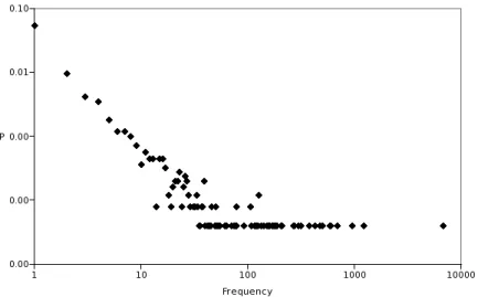
Figure 1 shows the distribution of the occupations in the whole population of the database which can be approximated by a power law1.
We will now try and explain this property of the distribution by studying the dynamics of the system. In other words, we will address the question of how a man chooses its own occupation, knowing the occupation of his father and of other people around him.
However, we will not consider people individually but within a given period of time (actually the data is given within 1-year periods of time, and one can also want to consider longer historical periods).
The dynamics will be decomposed as follows.
1. First of all, there is a non-negligeable probability that a man may ‘inherit’ the occupation of his father.
1Only the sons are considered here, to avoid counting a man once as a son and then
possibly several times as the father of several sons. Actually, a similar bias remains since many men were to marry more than once due to a high mortality rate. Anyway, none of these problems are likely to have a serious impact on the power-law distribution (which remains similar whether fathers are added or not to the whole population).
Figure 1: Distribution of the occupations in the database.
The Y-axis gives the probabilities, for an occupa-tion, to have the frequency given on the X-axis. Both scales are logarithmics.
2. Now if this is not the case, one may take as an initial guess that he will choose an occupation with a probability following the distribution of people among all existing occupations. This is the very principal of preferential attachment.
2.2
Formalization
As explained above, time will be considered discrete, ranging from 1 to a given integer T . The set of existing occupations over the whole set of time periods will also be denoted by integers from 1 to the cardinality n of the set of occupations. Given a time period, the data can thus be seen as a so-called mobility matrix (see below) M ∈ Nn×n in which a row (resp. a column) numbered i gives the
distribution of occupations of all the sons (resp. fathers) having fathers (resp. sons) with occupation i. The integer Mi,j is thus the number of sons having
occupation j and whose father has occupation i.
Definition 1 (mobility matrix) Given a discrete property ranging from 1 to an integer n, we will call mobility matrix of size n a matrix of dimension n × n with non-negative integer values.
Note that the time period is not written in order to simplify the notations. In all the notations defined below, a given time period is understood.
The total number of sons (which is equal to the total number of fathers due to the nature of the data, see note 1, p. 2) will be denoted p (for ‘population’). The distribution of occupations among the sons (resp. fathers) will be de-noted as a Nnvector S (resp. F) for plain values (S
iis the number of sons having
occupation i) and as a [0, 1]n normalized vector ψ (resp. φ) for probabilities (ψ i
The number of sons having taken the occupations of their fathers can be read on the diagonal of the matrix M, which will be denoted D ∈ Nn as a vector, D
i
being the number of sons whose occupation is i as well as their fathers. Conversely, the number of sons having occupation i unlike their fathers is obtained by substracting Di (the i-th diagonal value of matrix M) to the sum
of values on the i-th column of M. They will be denoted with a vector A. The following table sums up the notations used in the paper.
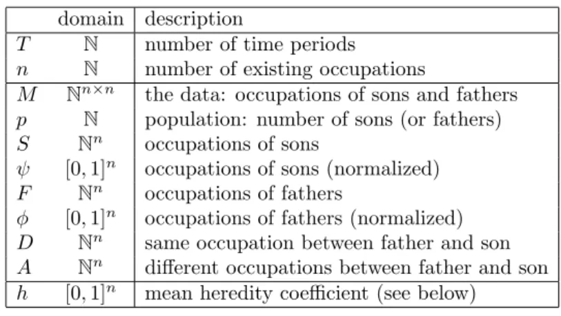
domain description
T N number of time periods
n N number of existing occupations
M Nn×n the data: occupations of sons and fathers p N population: number of sons (or fathers) S Nn occupations of sons
ψ [0, 1]n occupations of sons (normalized)
F Nn occupations of fathers
φ [0, 1]n occupations of fathers (normalized)
D Nn same occupation between father and son
A Nn different occupations between father and son
h [0, 1]n mean heredity coefficient (see below)
2.3
Heredity
We will now look at the first part of the dynamics sketched above.
Definition 2 (heredity coefficient) Given a discrete property ranging from 1 to an integer n, and a mobility matrix M of size n, the heredity coefficient of the (non-zero positive) value i ≤ n is the ratio between the i-th diagonal value and the sum of the i-th column:
her(i) = PnMi,i j=1Mj,i
.
The mean heredity coefficient is the ratio between the sum of diagonal values and the sum of all values of the matrix.
In the case of our professional mobility matrices (one matrix for each time period), the heredity coefficient of an occupation i in a given time period is the amount of sons having kept the occupation of their fathers among all sons having occupation i. The mean heredity coefficient is the amount of sons having the same occupation as their fathers.
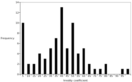
Figure 2 shows the distribution of heredity coefficients for occupations with at least 10 fathers and 10 sons2in a 20-year time period, and the mean heredity coefficient for the whole time period. Two observations can be made:
• the distribution is symmetric with a significant average value ;
• this average value is quite high, which means that the first part of the dynamics described above is important.
2keeping all occupations leads to artifacts in the distribution (like high peaks in values 0, 1
3, 1 2,
2
Figure 2: Distribution of heredity coefficients in time period 1843–1862.
Here the mean heredity coefficient is 0.42
2.4
Preferential attachment?
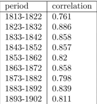
We will now look at the second part of the dynamics and focus on the sons that have chosen another occupation than the one of their fathers. To test the ‘guess’ made above, one may look at the extent in which vector A of a given time period is correlated with vector S of the former time period. Figure 3 shows these measures of correlations.
The correlation coefficients obtained in the previous experiment are quite good and thus partly validate the dynamics sketched above, even though they could perhaps be stronger, and we will come to this later.
2.5
A nice formula
It can be noted that the distributions of occupations among fathers and among sons are highly correlated, as can be seen on Figure 4.
One can thus try and express the dynamics only in terms of the occupations of sons and fathers in one given time period.
The description given above of the distribution of heredity coefficients of the occupations allows us to make a first approximation, assuming all occupations have the same heredity coefficient h which is the mean heredity coefficient.
period correlation 1813-1822 0.761 1823-1832 0.886 1833-1842 0.858 1843-1852 0.857 1853-1862 0.82 1863-1872 0.858 1873-1882 0.798 1883-1892 0.839 1893-1902 0.811
Figure 3: Correlations between sons on all 10-year time periods.
The value given for each period is the av-erage correlation between the two vectors of sons’occupations in the current time period and in the previous one
period correlation 1801-1837 0.8
1838-1861 0.77 1862-1883 0.74 1884-1902 0.75
by definition: Si = Mi,i+ X 1 ≤ j ≤ n j 6= i Mj,i = her(i) × Fi+ X 1 ≤ j ≤ n j 6= i Mj,i
which can be approximated by: Si ≈ hFi+ X 1 ≤ j ≤ n j 6= i Fj× Mj,i Fj .
By using the vector notation, this approximation can be rewritten as follows (product of matrices by vectors is denoted here with ×, and product by scalar with a dot (·)):
S ≈ F × (h · I + m), (1) where I is the identity matrix and m the following:
m = 0 M1,2 F1 · · · M1,n F1 M2,1 F2 0 · · · M2,n F2 .. . ... ... Mn,1 Fn Mn,2 Fn · · · 0 (2)
(the 0’s are only on the diagonal.)
Now, taking into account the second part of the dynamics, we can make the following approximation for a given occupation i in a given time period:
Si≈ hFi+ ψi×
X 1 ≤ j ≤ n
j 6= i Fj,
which can again be simplified by considering as highly correlated the vectors ψ and φ (thus probabilities of having occupation i, for a son ψi and for a father
φi): Si≈ hFi+ φi× X 1 ≤ j ≤ n j 6= i Fj.
This latter approximation gives the same general formula (1) as before, but with the following matrix:
m = 0 φ2 · · · φn φ1 0 · · · φn .. . ... ... φ1 φ2 · · · 0 (3)
We will look, with this formula, at two other systems in which power-law distributions can be found.
3
Family names
The distribution of family names among a given population can usually be approximated by a power law, as can be seen on Figure 5.
In many cultures, family names are transmitted in the following way : • men and unmaried women get most of the time the name of their fathers ; • a married woman takes the name of her husband.
This leads to the following dynamics, for each generation: • more than half of the people keep the name of their fathers ;
• the rest of the people get a name with a probability following the distri-bution of names among the whole population.
Here equation 1 can still approximate the dynamics of the system, with a new meaning for F and S (names of fathers and children rather than occupations of fathers and sons).
4
Cities
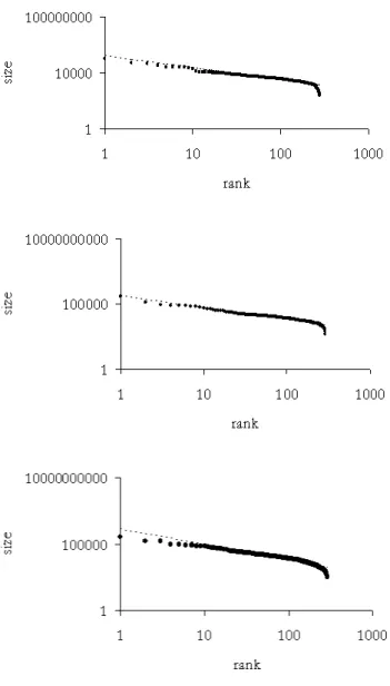
The distribution of the dimensions of cities (or geographic areas) in terms of their population can also be approximated by a power law, as can be seen in Figure 6.
Studies on migrations have shown that the intensity of migration between one city and another depends on both the population of the two cities and on the distance between them. This idea was formalized with the following so-called gravitational law [You28, Car58, Zip49, Leb00] (stated here with the same notations as in the case of occupations in order to stress the similarities between the two cases).
Property 1 (gravitational law) Let 1, . . . , n be a set of cities, F∈Nn be the vector of their populations in the beginning of a given time period, and let d(i, j) denote an (Euclidean) distance between i and j. Then there is a factor k ∈ R (depending on the time period and on the distance used) such that the number of people leaving a city i ≤ n for another city j ≤ n, j 6= i, can be approximated by:
µ(i, j) = k ·Fi· Fj d(i, j).
The dynamics here is a bit more complex than in the case of family names. In each period of time, we have the following two cases.
• In each city, there is a certain (important) proportion of people remaining in the same city as in the former period.
Figure 5: Distribution of Florentine names in 1427, 1810 and 2001.
The distribution charts are read the same way as in Figure 1.
Figure 6: Population of Tuscan districts in 1810, 1951 and 2001.
Here, the charts give the size of the first, then second, then . . . districts (that are actual towns in the 20th century).
• People moving from a city to another one ‘choose’ the new one with a probability given by the so-called gravitational law stated above, depend-ing on the distance and on the distribution of people among all cities. According to the gravitational law, the number of people coming to a given city i among n cities during a given time period can be approximated by the following value: in(i) = k · X 1 ≤ j ≤ n j 6= i FjFi d(i, j) = k p· X 1 ≤ j ≤ n j 6= i Fj· φi d(i, j),
where d is a distance function and k ∈ R a constant depending on the time period and on the distance function.
Equation 1 can still sketch the process (with, again, a new meaning for F and S as the distribution of people in a city at the beginning and at the end of a time period), but with the following matrix:
m = k0· 0 φ2 d(1,2) · · · φn d(1,n) φ1 d(2,1) 0 · · · φn d(2,n) .. . ... ... φ1 d(n,1) φ2 d(n,2) · · · 0 , (4)
k0 ∈ R depending on the time period and on the distance d used.
5
A network of social proximities
5.1
Distances between occupations?
Back to the professional occupations, the idea of the distances is obviously rel-evant. Of course, the probability that a man will choose a given occupation depends not only on the amount of people having this occupation. It depends also strongly on the proximity of this occupation to his social status and envi-ronment.
Comparison of matrices (2) and (4) yields a way to ‘extract’ from the data of professional mobilities (a kind of) distances between occupations that can be computed as follows, given a time period:
dist(i, j) = φjFi Mi,j
, provided Mi,j6= 0.
5.2
Proximities rather than distances
Note that another way to understand the definition of dist() is to compare matrices (3) and (2): dist(i, j) is indeed a measure of the accuracy of the ap-proximation made using preferential attachment. A value much greater than 1 means that the effective value found in the data matrix is much less than the one expected with the approximation, whereas a value much smaller than 1 (always nonnegative however), means on the contrary that the effective value is much greater than expected.
Actually, this latter case is the most relevant one since our matrices are sparse (the data as well as the approximation matrices) and very low values are common (especially 0 in the data). The greater a value is, the more statistically significant it is. It is thus more relevant to talk about proximities rather than distances and invert the formula by defining the following function:
prox(i, j) = Mi,j φjFi
,
whose higher values will stress professional mobilities that are more often ob-served than was expected.
Note that using this new definition solves two formal incongruities of the definition of dist(): first, dist() is not a distance. Second, this enables us to use 0 for Mi,j. A proximity value of 0 between i and j just means that no son with
occupation j has been found whose father has occupation i.
5.3
An example
When calculating the proximities matrix for a given time period (namely 1843– 1852), we get the (far) highest values for ‘self-loops’ of the network, i.e. diagonal values3, which is a confirmation of the importance of the heredity part in the
dynamics.
Putting aside diagonal values, we also get high values for some links whose ‘destinations’ are occupations typical of the beginning of a career (and thus much more common among sons than among fathers). This is of course the limitation of the approximation made by using φ rather than ψ (see Section 2.5). Although highly correlated, these two distributions (occupations of fathers and of sons) much differ in some points like the ones described here. As an example, in the considered time period, servants are only 7 among fathers while 108 among sons. However, looking closer to the links having servant as their destination, we can see an interesting phenomenon. The greatest proximity value is for the link coming from day labourer, which is an occupation with quite the same probability among fathers and sons. The proximity value of this link is almost twice as high as the next link in the list (in proximity inverse order), coming from ploughman. Moreover, the link day labourer – servant is the far most common link among those coming from day labourer.
One could thus make the following conjecture: this link is a kind of ‘hered-itary’ link, in the sense that day labourer might be the usual evolution of a servant when he gets to the age of his father.
3Of course diagonal values are not supposed to be considered here, but applying the formal
This ‘naive’ remark coming only from the observation of the data meets issues addressed in existing studies about servants [Sar01, Sal04, Sal05].
6
Conclusion
The example given in the last section illustrates the kind of usage that can be done of the function of proximity, whose aim is to put into evidence attractions between nodes of a network that are hidden by high numbers.
This technique can be used on many valued networks: the WWW to find out proximities between websites taking into account their popularities (the number of links from a website s to another one t can be quite low, but be considered high if t is almost unknown of the rest of the web), e-mail exchanges between individuals, data exchange on peer-to-peer networks etc.
Acknowledgements
We are grateful to Jean-Pierre P´elissier to have let us use the database and also thank Maurizio Gribaudi for many discussions about it.
This work is partly supported by the french ACI fundings Syst`emes com-plexes en SHS and Usages de l’Internet, by way of the PERSI working group4.
References
[BA99] A.-L. Barabasi and R. Albert. Emergence of scaling in random net-works. Science, 1999.
[Boi74] J. Boissevain. Friends of Friends, Networks, Manipulators and Coalitions. Basil Blackwell, Oxford, 1974.
[Bou80] P. Bourdieu. Le capital social. notes provisoires. Actes de la recherche en sciences sociales, 31:2–3, 1980.
[Bur04] R. Burt. Structural holes and good ideas. American Journal of Sociology, 2004.
[Car58] V. Carrothers. A historical review of the gravity and potential con-cepts of human relations. Journal of the American Institute of Plan-ners, XXII:94–102, 1958.
[Col88] J. Coleman. Social capital in the creation of human capital. Amer-ican Journal of Sociology, S.(94):95–120, 1988.
[DM03] S.N. Dorogovtsev and J.F.F. Mendes. Evolution of Networks: From Biological Nets to the Internet and WWW. Oxford University Press, 2003.
[FFF99] M. Faloustos, P. Faloustos, and C. Faloustos. On power-law relation-ships of the internet topology. In Proceedings of the ACM SIGCOMM ’99 Conference. ACM, New-York, 1999.
[FKP02] Fabrikant, Koutsoupias, and Papadimitriou. Heuristically optimized trade-offs: A new paradigm for power laws in the internet. In ICALP: Annual International Colloquium on Automata, Languages and Programming, 2002.
[Gab99] X. Gabaix. Zipf’s law for cities: an explaination. Quarterly Journal of Economics, 114:739–767, 1999.
[KRR+00] Kumar, Raghavan, Rajagopalan, Sivakumar, Tomkins, and Upfal. Stochastic models for the web graph. In FOCS: IEEE Symposium on Foundations of Computer Science (FOCS), 2000.
[KRRT99] S. R. Kumar, P. Raghavan, S. Rajagopalan, and A. Tomkins. Ex-tracting large-scale knowledge bases from the web. In Proceedings of the 25th VLDB Conference. 1999.
[Leb00] H. Lebras. Essai de g´eom´etrie sociale. Odile Jacob, 2000.
[New03] M. E. J. Newman. The structure and function of complex networks. SIAM Review, 167(45), 2003.
[Par96] V. Pareto. Cours d’ ´Economie Politique. Dronz, Geneva, 1896. [Sal04] G. Salinari. Anatomia di un gruppo senza storia: i domestici a
firenze (1810–1875). Polis, XVIII:47–75, 2004.
[Sal05] G. Salinari. La montagne et la ville. In S. Palseau and I. Schopp, editors, Proceedings of the Servant Project, volume II. Les Editions de l’Universit´e de Li`ege, 2005. to appear.
[Sar01] R. Sarti. ”noi abbiamo visto tante citt`a, abbiamo un’altra cultura”. servizio domestico, migrazioni e identit`a di genere in italia: uno sguardo di lungo periodo. Polis, XVIII:17–46, 2001.
[Wat03] Duncan Watts. Six Degrees: The Science Of A Connected Age. W.W.Norton, London, 2003.
[You28] E. C. Young. The movement of farm population. Cornell Agriculture Experimental Station Bull. 426, 1928.
[Zip49] G. K. Zipf. Human Behaviour and the Principle of Least Effort. An Introduction to Human Ecology. Addison-Wesley, Cambridge, Ma, 1949.