HAL Id: inserm-00274332
https://www.hal.inserm.fr/inserm-00274332
Submitted on 18 Apr 2008HAL is a multi-disciplinary open access archive for the deposit and dissemination of sci-entific research documents, whether they are pub-lished or not. The documents may come from teaching and research institutions in France or abroad, or from public or private research centers.
L’archive ouverte pluridisciplinaire HAL, est destinée au dépôt et à la diffusion de documents scientifiques de niveau recherche, publiés ou non, émanant des établissements d’enseignement et de recherche français ou étrangers, des laboratoires publics ou privés.
Computing normalised prediction distribution errors to
evaluate nonlinear mixed-effect models: The npde
add-on package for R.
Emmanuelle Comets, Karl Brendel, France Mentré
To cite this version:
Emmanuelle Comets, Karl Brendel, France Mentré. Computing normalised prediction distribution errors to evaluate nonlinear mixed-effect models: The npde add-on package for R.. Computer Meth-ods and Programs in Biomedicine, Elsevier, 2008, 90 (2), pp.154-66. �10.1016/j.cmpb.2007.12.002�. �inserm-00274332�
Computing normalised prediction distribution errors to evaluate nonlinear
mixed-effect models: the npde add-on package for R
Emmanuelle Comets1,2, Karl Brendel3, France Mentré1,2,4
1INSERM, U738, Paris, France
2Université Paris 7, UFR de Médecine, Paris, France
3Institut de Recherches Internationales Servier, Courbevoie, France 4AP-HP, Hôpital Bichat, UF de Biostatistiques, Paris, France
Corresponding author: Emmanuelle Comets
INSERM U738, Université Paris 7 UFR de Médecine, site Bichat 16 rue Henri Huchard
75 018 Paris, France Tel: (33) 1.44.85.62.77. Fax: (33) 1.44.85.62.80.
Email: emmanuelle.comets@bichat.inserm.fr
J
OURNAL
:
Computer Methods and Programs in Biomedicine
S
ECTION
:
Systems and Programs
HAL author manuscript inserm-00274332, version 1
HAL author manuscript
K
EYWORDS
• population pharmacokinetics • population pharmacodynamics • model evaluation
• nonlinear mixed-effects model • npde
Number of figures: 9
Number of tables: 2
A
BSTRACT
Pharmacokinetic/pharmacodynamic data are often analysed using nonlinear mixed-effect models, and model evaluation should be an important part of the analysis. Recently, normalised prediction distribution errors (npde) have been proposed as a model evaluation tool. In this paper, we describe
an add-on package for the open source statistical package R, designed to compute npde. npde take
into account the full predictive distribution of each individual observation and handle multiple ob-servations within subjects. Under the null hypothesis that the model under scrutiny describes the validation dataset, npde should follow the standard normal distribution. Simulations need to be per-formed beforehand, using for example the software used for model estimation. We illustrate the use of the package with 2 simulated datasets, one under the true model and one with different parameter values, to show how npde can be used to evaluate models. Model estimation and data simulation were
performed usingNONMEMversion 5.1.
1
Introduction
The analysis of longitudinal data is prominent in pharmacokinetic (PK) and pharmacodynamic (PD) studies, especially during drug development [1]. Nonlinear mixed-effect models are increas-ingly used as they are able to represent complex nonlinear processes and to describe both between and within subject variability. The evaluation of these models is gaining importance as the field of their application widens, ranging from dosage recommendation to clinical trial simulations [2]. Fol-lowing the definition of Yano et al. [2]: "the goal of model evaluation is objective assessment of the predictive ability of a model for domain-specific quantities of interest, or to determine whether the model deficiencies (the final model is never the ‘true model’) have a noticeable effect in substantive inferences."
Despite the recommendations of drug agencies [3, 4] stressing the importance of model evalua-tion, a recent survey based on all published PK and/or PD analyses over the period of 2002 to 2004 shows that it is infrequently reported and often inadequately performed [5]. One possible explana-tion is the lack of consensus concerning a proper evaluaexplana-tion method. Following the development of linearisation-based approaches for the estimation of parameters in nonlinear mixed-effect models, standardised prediction errors [6] have been widely used as diagnostic tools, not the least because they
were computed in the main software used in population PKPD analyses,NONMEM[7], where they are
reported under the name weighted residuals (WRES). However, because of the linearisation involved in their computation there is no adequate test statistic. In 1998, Mesnil et al. proposed prediction dis-crepancies, which were easily computed due to the discrete nature of the non-parametric distribution estimated, to validate a PK model for mizolastine [8]. Prediction discrepancies (pd) are defined as the percentile of an observation in the predictive distribution for that observation, under the null
hy-pothesis (H0) that the model under scrutiny adequately describes a validation dataset. The predictive
distribution is obtained assuming the posterior distribution of the estimated parameters by maximum likelihood estimation, disregarding the estimation error (the so-called plug-in approach [9]). By con-struction pd follow a uniform distribution over [0,1], providing a test. In the Bayesian literature this idea of using the whole predictive distribution for model evaluation has been proposed by Gelfand et al [10] and is also discussed by Gelman et al [11]. Yano et al. extended this notion in a non-Bayesian framework, proposing the approach known as Posterior Predictive Check (PPC) [2], while Holford advocated a more visual approach under the name Visual Predictive Check (VPC) [12]. Mentré and Escolano [13] discuss how prediction discrepancies relate to one of the three forms of PPC described by Yano. For non-discrete distributions, Mentré and Escolano proposed to compute prediction dis-crepancies by Monte-Carlo integration [14, 13]. In their original version, pd however did not take into account the fact that subjects usually contributes several measurements which induces correlations be-tween pd, leading to increased type I error. This was improved in a further work, and the uncorrelated and normalised version of pd was termed normalised prediction distribution errors (npde) [15]. npde have better properties than WRES, and can also be used to evaluate covariate models [16]. They can be used for internal or external evaluation, depending on whether they are computed on the dataset used to build the model (internal evaluation) or on an external dataset.
The computation of the npde however requires some programming. We therefore developed an
add-on package, npde, for R, the open source language and environment for statistical computing
and graphics [17], to enable easy computation of the npde [18]. Other packages such asXpose[19],
for diagnostic and exploration, andPFIM[20, 21], for the evaluation and optimisation of population
designs, have been developed inRfor the analysis of population PK and/or PD studies. Xposeis very
useful as an aid for model assessment and run management for studies performed with theNONMEM
software [7], widely used in this field but with next to no plotting capabilities, so that Rwas a good
choice of language for the implementation ofnpde.
In section 2, we briefly recall how npde are computed. In section 3 we describe the main features and usage of the package. In section 4 we illustrate the use of the package with two simulated examples. The examples are simulated based on the well known dataset theophylline, available both in R andNONMEM: the first (Vtrue) is simulated with the model used for the evaluation, while the
second (Vfalse) is simulated assuming a different set of parameters, and we show how npde can be
used to reject the model for Vfalse but not for Vtrue.
2
Computational method and theory
2.1
Models and notations
Let B denote a building (or learning) dataset and V a validation dataset (V can be the same as B for
internal evaluation). B is used to build a population model called MB. Evaluation methods compare
the predictions obtained by MB, using the design of V, to the observations in V. V can be the learning
dataset B (internal evaluation) or a different dataset (external evaluation). The null hypothesis (H0) is
that data in the validation dataset V can be described by model MB.
Let i denote the ith individual (i = 1,..., N) and j the jth measurement in an individual ( j = 1,..., ni,
where niis the number of observations for subject i). Let ntot denote the total number of observations
(ntot =∑ini ). Let Yi be the ni-vector of observations observed in individual i. Let the function f
denote the nonlinear structural model. f can represent for instance the PK model. The statistical
model for the observation yi j in patient i at time ti j, is given by:
yi j= f (ti j,θi) +εi j (1)
whereθiis the vector of the individual parameters andεi j is the residual error, which is assumed to
be normal, with zero mean. The variance ofε may depend on the predicted concentrations f(t ,θ)
through a (known) variance model. Letσdenote the vector of unknown parameters of this variance model.
In PKPD studies for instance, it is frequently assumed that the variance of the error follows a combined error model:
var(εi j) =σ2inter+σ2slope f(ti j,θi)2 (2)
whereσinterandσslopeare two parameters characterising the variance. In this case,σ= (σinter,σslope)′.
This combined variance model covers the case of an homoscedastic variance error model, where
σslope= 0, and the case of a constant coefficient of variation error model whenσinter= 0.
Another usual assumption in PKPD analyses is that the distribution of the individual parameters
θifollows a normal distribution, or a log-normal distribution, as in:
θi= h(µ, Xi) eηi (3)
where µ is the population vector of the parameters, Xia vector of covariates, h is a function giving the
expected value of the parameters depending on the covariates, andηirepresents the vector of random
effects in individual i. ηi usually follows a normal distribution
N
(0,Ω), whereΩ is thevariance-covariance matrix of the random effects, but other parametric or non-parametric assumptions can be used for the distribution of the random effects, as in the first paper proposing prediction discrepancies in the context of non-parametric estimation [8]. Although npde were developed in the area of PK and PD analyses, they are a general way of evaluating mixed-effect models and require only observations and corresponding predicted distributions.
We denote P the vector of population parameters (also called hyperparameters) estimated using
the data in the learning dataset B: P= (µ′, vect(Ω)′,σ′)′, where vect(Ω) is the vector of unknown
values inΩ. Model MB is defined by its structure and by the hyperparameters ˆPBestimated from the
learning dataset B.
2.2
Definition and computation of npde
Let Fi j denote the cumulative distribution function (cdf) of the predictive distribution of Yi j under
model MB. We define the prediction discrepancy pdi j as the value of Fi j at observation yi j, Fi j(yi j).
Fi j can be computed using Monte-Carlo simulations.
Using the design of the validation dataset V, we simulate under model MB K datasets Vsim(k)
(k=1,...,K). Let Ysimi (k)denote the vector of simulated observations for the ith subject in the kth
simu-lation.
pdi j is computed as the percentile of yi j in the empirical distribution of the ysimi j (k):
pdi j= Fi j(yi j) ≈ 1 K K
∑
k=1 δi jk (4)whereδi jk= 1 if ysimi j (k)< yi j and 0 otherwise.
By construction, prediction discrepancies (pd) are expected to follow
U
(0, 1), but only in the caseof one observation per subject; within-subject correlations introduced when multiple observations are available for each subject induce an increase in the type I error of the test [13]. To correct for this
correlation, we compute the empirical mean E(Yi) and empirical variance-covariance matrix var(Yi)
over the K simulations. The empirical mean is obtained as:
E(Yi) = 1 K K
∑
i=1 Ysimi (k)and the empirical variance is:
var(Yi) = 1 K− 1 K
∑
i=1(Yisim(k)− E(Ysimi (k)))(Yisim(k)− E(Ysimi (k)))′
We use thevarfunction from R to provide unbiased estimates of var(Yi).
Decorrelation is performed simultaneously for simulated data:
sim(k)∗ −1/2 sim(k)
and for observed data:
Y∗i = var(Yi)−1/2(Yi− E(Yi))
Decorrelated pd are then obtained using the same formula as in (4) but with the decorrelated data, and we call the resulting variables prediction distribution errors (pde):
pdei j = Fi j∗(y∗i j) ≈ 1 K K
∑
k=1 δ∗ i jk (5) whereδ∗i jk= 1 if ysimi j (k)∗< y∗ i j and 0 otherwise.Sometimes, it can happen that some observations lie either below or above all the simulated data
corresponding to that observation. In this case, we define the corresponding pdei j as:
pdei j = 1/K if yi j < y sim(k) i j ∀k 1− 1/K if yi j > ysimi j (k) ∀k (6)
Under H0, if K is large enough, the distribution of the prediction distribution errors should follow
a uniform distribution over the interval [0,1] by construction of the cdf. Normalised prediction distri-bution errors (npde) can then be obtained using the inverse function of the normal cumulative density function implemented in most software:
npdei j=Φ−1(pdei j) (7)
By construction, if H0 is true, npde follow the
N
(0, 1) distribution without any approximation andare uncorrelated within an individual.
2.3
Tests and graphs
Under the null hypothesis that model MB describes adequately the data in the validation dataset,
the npde follow the
N
(0, 1) distribution. We use 3 tests to test this assumption: (i) a Wilcoxon signedrank test, to test whether the mean is significantly different from 0; (ii) a Fisher test for variance, to
test whether the variance is significantly different from 1; (iii) a Shapiro-Wilks test, to test whether the distribution is significantly different from a normal distribution. The package also reports a global test, which consists in considering the 3 tests above with a Bonferroni correction. The p-value for this global test is then reported as the minimum of the 3 p-values multiplied by 3 (or 1 if this value is larger than 1) [22]. Before these tests are performed, we report the first three central moments of the distribution of the npde: mean, variance, skewness, as well as the kurtosis, where we define kurtosis
as the fourth moment minus 3 so that the kurtosis for
N
(0, 1) is 0 (sometimes called excess kurtosis).The expected value of these four variables for
N
(0, 1) are respectively 0, 1, 0 and 0. We also givethe standard errors for the mean (SE=s/√ntot) and variance (SE=s2p2/(ntot− 1)) (where s is the
empirical variance).
Graphs can be used to visualise the shape of the distribution of the npde. The following graphs are plotted by default: (i) QQ-plot of the npde (the line of identity is overlaid, and the npde are expected to fall along along this line) (ii) histogram of the npde (the density line of the expected
N
(0, 1) is overlaid to show the expected shape), scatterplots of (iii) npde versus X and (iv) npdeversus predicted Y, where we expect to see no trend if H0 is true. For the last plot, the package
computes for each observation the predicted Y as the empirical mean over the k simulations of the
simulated predicted distribution (denoted E(ysimi j (k))), which is reported under the name ypred along
with the npde and/or pd.
3
Program description
3.1
Overview
The program is distributed as a add-on package or library for the free statistical software R. A
guide for the installation ofRand add-on packages such asnpdecan be found on the CRAN
(Com-prehensive R Archive Network) at the following url: http://cran.r-project.org/. Ris available free of
charge and runs on all operating systems, which made it a very convenient language for the
develop-ment ofnpde. The package requires only observed and simulated data to compute the npde, and does
not use the model itself.
The npde library contains 14 functions. Figure 1 presents the functions hierarchy starting with
functionnpde. A similar graph is obtained with functionautonpdewithout the call to function
pde-menu.
An additional function (plotpd) can be called directly by the user to plot diagnostic graphs
involv-ing the prediction discrepancies instead of the npde, and is therefore not represented on the graph. The functions for skewness and kurtosis were modified from the two functions of the same name
proposed in thee1071package for R [23].
The methods described in section 2 are implemented as follows. Observed and simulated data are read in two matrices. For each subject, the empirical mean and variance of the simulated data
are computed using the Rfunctions mean, apply and cov. The inverse square root of the variance
matrix is obtained by the Cholesky decomposition using the functionscholandsolve. The remaining
computations involve matrix and vector multiplications. All these functions are available in the R
program.
The documentation contains the simulated examplesvtrue.datandvfalse.dat, as well as the
origi-nal data file and the control files used for estimation and simulation. The simulated datasimdata.dat
used to compute the npde for both simulated datasets can be downloaded from the website.
3.2
Preparing the input
The package needs two files: the file containing the dataset to be evaluated (hereafter named ’ob-served data’) and the file containing the simulations (hereafter named ’simulated data’). The package
does not perform the simulations. R, NONMEM[7], MONOLIX[24] or another program can be used
for that purpose, and the two following files should be prepared beforehand.
Observed data: the observed data file must contain at least the following three columns: id (patient
identification), xobs (design variable such as time, X, ...), yobs (observations such as DV, concentra-tions, effects...). An additional column may be present in the dataset to indicate missing data (MDV). In this case, this column should contain values of 1 to indicate missing data and 0 to indicate observed
data (as inNONMEMorMONOLIX). Alternatively, missing data can be coded using a dot (’.’) or the
character string NA directly in the column containing yobs. The computation of the npde will remove missing observations.
Other columns may be present but will not be used by the library. The actual order of the columns is unimportant, since the user may specify which column contain the requested information, but the default order is 1=id, 2=xobs, 3=yobs and no MDV column. A file header may be present, and column separators should be one of: blank space(s), tabulation mark, comma (,) or semi-colon (;).
Simulated data: the simulated data file should contain the K simulated datasets stacked one after
the other. Within each simulated dataset, the order of the observations must be the same as within the
observed dataset. The dimensions of the two datasets must be compatible: if nobs is the number of
lines in the observed dataset, the file containing the simulated datasets must have K×nobslines. The
simulated data file may contain a header but not repeated headers for each simulated dataset.
The simulated data file must contain at least 3 columns, in the following order: id (patient iden-tification), xsim (independent variable), ysim (dependent variable). The column setup is fixed and cannot be changed by the user, contrary to the observed data. Additional columns may be present but will not be used by the package. The id column must be equal to K times the id column of the observed dataset, and the xsim column must be equal to K times the xobs column of the observed dataset. If missing data is present in the observed data, they should be present in the simulated datasets and the corresponding lines will be removed for all simulated datasets during the computation.
Examples of a simulated and observed dataset are available in the subdirectory doc/inst of the
library.
BQL data: BQL (below the quantification limit LOQ) or otherwise censored data are currently
not appropriately handled by npde. If a maximum likelihood estimation method taking censored
data into account has been used for the estimation, these data should be removed from the dataset
or set to missing, using for example an MDV item, pending future extensions ofnpde. On the other
hand, if BQL data were set to LOQ or LOQ/2, they should remain in the dataset. npde will likely detect model misspecification related to these data, and we suggest to remove times for which too many observations are BQL before computing npde, since otherwise they might bias the results of the tests. During the simulations, negative or BQL data may be simulated due to the error model. At present, these values should be kept as is because the decorrelation step requires the whole predictive distribution. A transform both sides approach or the use of a double exponential model can be used to avoid simulating negative concentrations but this will not solve the BQL problem..
3.3
Computing npde
The package provides a function called npde to enter an interactive menu where the user is
prompted to enter the names of the files and the value of the different parameters required to com-pute npde. The menu is self-explanatory, and help pages are provided to understand the meaning of the different parameters. Fig. 3 shows an example of using this function (text entered by the user is shown in bold grey). The example will be detailed in section 4. The package checks the names that are provided and prompts the user for a new name if the corresponding file cannot be found.
Optionally, pd can also be computed. Although pd do not take multiple observations into ac-count [13], they are faster to compute than npde and can be used to perform diagnostics of model deficiencies. Also, when computation of npde fails due to numerical difficulties, an error message is printed and pd are computed instead (with corresponding plots). This problem can happen especially when model adequacy is very poor.
3.4
Output
During execution, the function prints the results of the tests described in methods (section 2.3).
An example of runningnpdecan be found in section 4.
In addition to the output printed on screen, three additional types of results are produced by
default: first, an R object containing several elements, including the npde and/or pd, is returned as
the value of the function; second, a graph file containing diagnostic plots of the npde is shown in the graphic window and saved in a file; third, the results are saved to a text file. Options are available so that the numerical results and graphs are not saved on disk, and so that the function returns nothing. Let us now discuss these three outputs in more detail.
The object returned by the function contains 7 elements: (i) a data frame obsdat containing the
observed data, with the following elements: id (patient ID), xobs (observed X) and yobs (observed
Y); (ii) ydobs: the decorrelated observed data y∗i j; (iii) ydsim: the decorrelated simulated data ysimi j (k)∗;
(iv) ypred: the predicted value. (v) xerr: an integer (0 if no error occurred during the computation); (vi) npde: the normalised prediction distribution errors; (vii) pd: the prediction discrepancies.
A graphic R window appears after the computation is finished, containing the 4 plots detailed in
section 2.3. These plots are saved to disk (unless boolsave=F). The name of the file is given by the
user (see Fig. 3), and an extension is added depending on the format of the graph (one of: Postscript, JPEG, PNG or PDF, corresponding to extensions .eps, .jpeg, .png and .pdf respectively).
The results are saved in a text file with the following columns: id (patient ID), xobs (observed X), ypred (predicted Y), npde, pd. The name of the file is the same as the name of the file in which graphs
are saved, with the extension.npde.
Sometimes the function is unable to compute the decorrelated prediction distribution errors for one or more subjects. This failure occurs during the decorrelation step and a warning message is printed on screen. When npde cannot be computed, the program computes automatically pd even if thecalc.pd=Foption was used. In this case, diagnostic graphs are plotted (see next section) but tests are not performed.
3.5
Other functions of interest
The npdefunction can be used to interactively fill in the required information. Alternatively, a
function calledautonpdeis provided, in which this information can be set as arguments. This function
requires 2 mandatory arguments: the name of the observed data file (or the name of theRdataframe);
and the name of the simulated data file (or the name of the R dataframe). A number of additional
optional arguments can be used to control message printing and output. These arguments and their
significance are given in Tab. 2. An example of a call toautonpdeis given in section 4.
A function calledplotnpdecan be used to plot the graphs described in the previous section. The arguments for this function are the observed X, the npde and the predicted Y (ypred). The function plotnpde is called byautonpde andnpde. A similar function, plotpd, can be used to plot diagnostic
plots for the pd. These include a QQ-plot of pd versus the expected uniform
U
(0, 1) distribution, ahistogram of the pd, and scatterplots of pd versus X and versus ypred.
The tests described in the previous section for npde can be performed using the functiontestnpde
(called byautonpdeandnpde). This function requires only the npde as argument.
4
Illustrative example
4.1
Data
To illustrate the use of the package, we simulated data based on the well known toy dataset record-ing the pharmacokinetics of the anti-asthmatic drug theophylline. The data were collected by Upton in 12 subjects given a single oral dose of theophylline who then contributed 11 blood samples over a period of 25 hours [7]. We removed the data at time zero from the dataset, and applied a one-compartment model with first-order absorption and elimination, as previously proposed [25]. The variability was modelled using an exponential model for the interindividual variability and a com-bined error model for the residual variability. The model was parameterised in absorption rate
con-stant ka(hr−1) volume of distribution V (L) and elimination rate constant k (hr−1) and did not include
covariates. Interindividual variability was modelled using an exponential model for the three PK
pa-rameters. A correlation between the parameters k and V was assumed (cor(ηk,ηV)). UsingNONMEM
(version 5.1) with theFOCE INTERACTIONestimation method, we obtained the parameter estimates
reported in Tab. 1. This model and these parameter estimates correspond to MB.
Vtrue was simulated under MB (H0), using the parameters reported in Tab. 1, while Vfalse (H1) was
simulated assuming a bioavailability divided by 2 (so that V/F is multiplied by 2). These datasets are
stored in two files called respectivelyvtrue.datandvfalse.dat. Fig. 2 show plots of the concentration
versus time profiles for the two datasets.
4.2
Simulation setup
The K simulations under MB, needed to compute the npde, were also performed usingNONMEM.
The control file used for the estimation was modified to set the values of the parameters (PK param-eters, variability and error model) to the values in Tab. 1, and the number of simulations was set to
K= 2000. The simulated data were saved to a file calledsimdata.dat.
The simulated data describes the predicted distribution for MB, so we use it to compute the npde
for both Vtrueand Vfalse.
4.3
Computing npde for V
trueThe functionnpdewas used to compute the npde for the simulated dataset Vtrue, and the results
were redirected to theRobjectmyres.truewith the following command:
myres.true<-npde()
Fig. 3 shows the set of questions (in black) answered by the user (in grey).
Fig. 4 shows the output printed on screen. The first four central moments of the distribution of
the npde are first given; here they are close to the expected values for
N
(0, 1), that is, 0 for themean, skewness and (excess) kurtosis and 1 for the variance. Then, the 3 tests for mean, variance and normality, as well as the adjusted p-value for the global test, is given. Here, none of the tests are significant. Fig. 5 shows the graphs plotted for npde. The upper left graph is a quantile-quantile
plot comparing the distribution of the npde to the theoretical
N
(0, 1) distribution, and the upper rightgraph is the histogram of the npde with the density of
N
(0, 1) overlayed. Both graphs show that thenormality assumption is not rejected. In the two lower graphs, npde are plotted against respectively time (the independent variable X) and predicted concentrations (predicted Y). These two graphs do not show any trend within the npde.
4.4
Computing npde for V
falseWe now use theautonpdefunction to compute the npde for the second dataset, Vfalse, setting the
parameters as arguments to the function with the following command:
myres.false<-autonpde("vfalse.dat","simdata.dat",1,3,4,namesav="vfalse", calc.pd=T)
Fig. 6 shows the output printed on screen and Fig. 7 shows the corresponding graphs. The graphs and the Shapiro-Wilks test show that the normality assumption itself is not rejected, but the test of the mean and variance indicate that the distribution is shifted (mean -0.45) and has an increased variance
(standard deviation 1.3) compared to
N
(0, 1). The scatterplots in the lower part of Fig. 7 also showsa clear pattern, with positive npde for low concentrations and negative npde for high concentrations, reflecting model misfit.
4.5
Influence of the number of simulations
A full study of the choice of the number of simulations (K), that should be performed with respect to the size of V, is beyond the scope of this paper. However, to assess the influence of the number of simulations on the results, we performed a small simulation study. Because the computation of the npde can be time-consuming, we simulated designs where all subjects have the same sampling
times and the same dose, and thus the same predicted distribution. The dose chosen was the median dose received by the actual patients (4.5 mg) and the 10 times were close to those observed (t={0.25, 0.5, 1, 2, 3.5, 5, 7, 9, 12, 24}). Then, we simulated the predicted distribution with K simulations
(K in {100, 200, 500, 1000, 2000, 5000}) and used the same var(Yi) and E(Yi)) to decorrelate the
vectors of observations for each simulated subject. To assess the influence of K for different designs, we simulated four different datasets, with N=12, 100, 250 and 500 subjects respectively. One set of
simulations was performed under H0while the other set of simulations was performed under the same
parameter assumptions as for Vfalse.
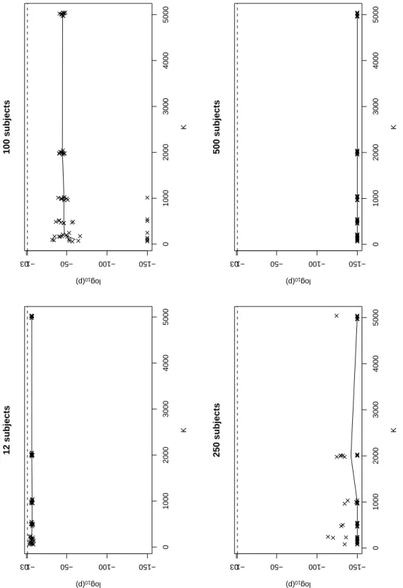
Figure 8 shows the base 10-logarithm of the p-values (log10(p)) obtained for the global test, for
the first set of simulations. The three tests (mean, variance, and normality) show the same qualitative
behaviour (data not shown). Each graph represents one simulated data set under H0 for N=12, 100,
250 and 500 subjects respectively. In the graphs, we represent log10(p) because for large number of
subjects, p-values become very small, and we jitterised the value of K by randomly adding a number between -50 and 50, so that the points would not be superimposed. In these graphs, we observe that small values of K are unreliable: for N=100, the scatter stabilises around K=1000, but for N=250
K=2000 appears to be necessary and even larger values should be used for N=500. When K is small
and N is large (here, N=100), we do not simulate enough concentrations to reliably describe the predicted distribution of the concentrations, and several observed concentrations may be ascribed the same value of npde, so that the normality test in particular often fails. When K increases, the variability in the p-values decreases and the mean p-value stabilises, but large number of subjects require large values of K. The program issues a warning when K is smaller than 1000, but even that may not be sufficient when dealing with very large databases. In particular, we see that for 500 subjects with 10 observations per subject, even K=5000 may not be sufficient. Further work is needed to give more specific recommendations.
The second set of simulations, under H1, is shown in figure 9 for the datasets simulated with 12,
100 and 250 subjects. For the simulations with 500 subjects and some of the simulations with 250 subjects, the p-value of the test was reported as 0 due to the numerical approximation involved in
the software so we fixed an arbitrary cut-off of log10(p) = −150. The model is strongly rejected
regardless of the value of K and N. With choice of model assumptions for Vfalse therefore the value
of K has little influence in rejecting the wrong model.
5
Concluding remarks
Model evaluation is an important part of modeling. Diagnostic graphs are useful to diagnose potential problems with models, and plots of (weighted) residuals versus independent variables or predicted concentrations are a major part of this diagnostic. Weighted residuals are computed using the dataset used for model estimation (internal evaluation) whereas standardised prediction errors are computed using a different dataset (external evaluation). The shortcomings of standardised predic-tion errors however have been publicised when improved approaches based on simulapredic-tions were made possible by the increasing computer power [13, 16]. Conditional weighted residuals have been pro-posed recently [26] but still suffer from the approximation involved. More sophisticated approaches now use simulations to obtain the whole predictive distribution. They include visual predictive check (VPC), which complement traditional diagnostic graphs and improve detection of model deficien-cies [12], as well as normalised prediction distribution errors. npde do not involve any approximation of the model function and therefore have better properties [15].
Concerning the evaluation of the npde, the posterior distribution of the parameters is assumed to be located only at the maximum likelihood estimate without taking into account the estimation error; this plug-in approach was shown to be equally efficient in a very simple pharmacokinetic setting [2].
Mentré and Escolano discuss the implications of this choice in more detail, noting in particular that there are debates in the Bayesian literature as to whether the plug-in approach may not actually be preferable in practice [13]. A second practical limitation consists in using a limited number of simula-tions to compute the npde. Based on the results of the simulation study (section 4.5), we recommend to use at least K=1000 but the actual number depends on the dataset involved, and should be increased when the dataset includes a large number of subjects. This will be investigated in more details in
fu-ture work onnpde.
Although the computation of npde is not difficult, it does require some programming ability. With
the package npde we provide a tool to compute them easily, using the validation dataset and data
simulated under the null hypothesis that model MB describes the validation dataset, with the design
of the validation dataset. A global test is performed to check whether the shape, location and variance parameter of the distribution of the npde correspond to that of the theoretical distribution. The tests based on npde have better properties than the tests based on pd [16], because of the decorrelation. However, the decorrelation does not make the observations independent, except when the model is
linear so that the joint distribution of the Yiis normal. For nonlinear models such as those under study,
more work is necessary to assess the statistical properties of the tests. In addition, the normality test appears very powerful, especially when the datasets become large. When a model is rejected, the QQ-plots and plots of npde versus time, predictions or covariates should therefore also be considered to assess whether, in spite of the significant p-value, the model may not be considered sufficient to describe the data. Graphs of the pd should also be plotted when investigating model deficiencies, since the decorrelation involved in the computation of the npde may sometimes smooth the plots and mask model misfit, and pd can then offer additional insight.
To combine the 3 tests, the Bonferroni procedure was preferred to the previously used Simes procedure based on the result of a simulation study, in which we found the type I error of the global
test to be close to 5% when using a Bonferroni correction [16]. The global test with a Simes correction
can be easily computed using the p-values returned by the function testnpde(). Default diagnostic
graphs and diagnostics are also plotted to check model adequacy. Other diagnostic graphs can be plotted, against covariates for instance, using the npde returned by the package. A current limitation
of npde concerns BQL concentrations, which the present version of npdedoes not handle properly.
Recently, estimation methods that handle censored data by taking into account their contribution to the log-likelihood were implemented in Nonmem [27] and Monolix [28], making them readily available
to the general user. In the next extension to npde, we therefore plan to propose and implement a
method to handle BQL data for models using these estimation methods. In the meantime, we suggest to remove times for which too many observations are BQL before computing npde, since otherwise they might bias the results of the tests. A column specifying which concentrations should be removed can be used for that purpose.
Simulations need to be performed before using the package. This was not thought to be prob-lematic since simulations can be performed easily with the most frequently used software in the field, NONMEM, with a minimal modification of the control file, or withMONOLIX, out of the box. The
simulations involved in the computation ofnpdeare the same as those needed to perform VPC [12].
There is however no clear test for VPC, although testing strategies have been evaluated based on quantiles [29], and in addition multiple observations per subject induce correlations in the VPC. On the other hand, npde have been decorrelated, and should follow the expected standard normal distri-bution, thus providing a one-step test of model adequacy. Another problem is that when each subject has different doses and designs, it may be difficult to make sense of VPC. An unbalanced design is not a problem with npde since simulations are used to obtain the predictive distribution for each observation using the design for each individual. This makes them a kind of normalised VPC.
As a recent review points out, npde should be considered as an addition to the usual diagnostic
metrics, and, as for all simulation-based diagnostics, care must be taken to simulate data reproducing the design and feature of the observed data [30]. In particular, caution must be exercised when features like BQL or missing data, dropouts, poor treatment adherence, or adaptive designs are present.
6
Availability
npde can be downloaded from http://www.npde.biostat.fr. The documentation included in the
package provides a detailed User Guide as well as an example of simulation setup, containing the NONMEMestimation and simulation control files, the observed and simulated datasets.
npdeis a package distributed under the terms of the GNU GENERAL PUBLIC LICENSE Version
2, June 1991.
Acknowledgments
The authors wish to thank Dr Saik Urien (INSERM, Paris) and Pr Nick Holford (University of Auck-land, New Zealand) for helpful discussions and suggestions.
Conflict of Interest Statement
Karl Brendel is an employee of Servier (Courbevoie, France).
R
EFERENCES
[1] L. Aarons, M. O. Karlsson, F. Mentré, F. Rombout, J. L. Steimer, A. van Peer, C. B. Experts, Role of modelling and simulation in Phase I drug development, Eur. J. Pharm. Sci. 13 (2001) 115–122.
[2] Y. Yano, S. L. Beal, L. B. Sheiner, Evaluating pharmacokinetic/pharmacodynamic models using the posterior predictive check, J. Pharmacokinet. Pharmacodyn. 28 (2001) 171–192.
[3] Food and Drug Administration, Guidance for Industry: Population Pharmacokinetics, FDA, Rockville, Maryland, USA (1999).
[4] Committee for Medicinal Products for Human Use, European Medicines Agency, Draft guide-line on reporting the results of population pharmacokinetic analyses, EMEA (2006).
[5] K. Brendel, C. Dartois, E. Comets, A. Lemenuel-Diot, C. Laveille, B. Tranchand, P. Girard, C. M. Laffont, F. Mentré, Are population pharmacokinetic and/or pharmacodynamic models adequately evaluated? A survey of the literature from 2002 to 2004, Clin. Pharmacokinet. 46 (2007) 221–234.
[6] S. Vozeh, P. Maitre, D. Stanski, Evaluation of population (NONMEM) pharmacokinetic param-eter estimates, J. Pharmacokinet. Biopharm. 18 (1990) 161–73.
[7] A. Boeckmann, L. Sheiner, S. Beal, NONMEM Version 5.1, University of California, NON-MEM Project Group, San Francisco (1998).
[8] F. Mesnil, F. Mentré, C. Dubruc, J. Thénot, A. Mallet, Population pharmacokinetics analysis of mizolastine and validation from sparse data on patients using the nonparametric maximum likelihood method, J. Pharmacokinet. Biopharm. 26 (1998) 133–161.
[9] M. Bayarri, J. Berger, P values for composite null models, J. Am. Statist. Assoc. 95 (2000) 1127–42.
[10] A. E. Gelfand, Markov chain Monte Carlo in practice, Chapman & Hall, Boca Raton (1996).
[11] A. Gelman, J. B. Carlin, H. S. Stern, D. B. Rubin, Bayesian Data Analysis, Chapman & Hall, London (1995).
[12] N. Holford, The Visual Predictive Check: superiority to standard diagnostic (Rorschach) plots,
14th meeting of the Population Approach Group in Europe, Pamplona, Spain (2005) Abstr 738.
[13] F. Mentré, S. Escolano, Prediction discrepancies for the evaluation of nonlinear mixed-effects models, J. Pharmacokinet. Biopharm. 33 (2006) 345–67.
[14] F. Mentré, S. Escolano, Validation methods in population pharmacokinetics: a new approach
based on predictive distributions with an evaluation by simulations, 10thmeeting of the
Popula-tion Approach Group in Europe, Basel, Switzerland (2001).
[15] K. Brendel, E. Comets, C. Laffont, C. Laveille, F. Mentré, Metrics for external model evaluation with an application to the population pharmacokinetics of gliclazide, Pharm. Res. 23 (2006) 2036–49.
[16] K. Brendel, E. Comets, F. Mentré, Normalised prediction distribution errors for the evaluation
of nonlinear mixed-effects models, 16th meeting of the Population Approach Group in Europe,
Copenhagen, Denmark (2007) Abstr.
[17] R Development Core Team, R: A language and environment for statistical computing, R Foun-dation for Statistical Computing, Vienna, Austria (2004).
[18] E. Comets, K. Brendel, F. Mentré, Normalised prediction distribution errors in R: the npde
li-brary, 16thmeeting of the Population Approach Group in Europe, Copenhagen, Denmark (2007)
Abstr 1120.
[19] E. N. Jonsson, M. O. Karlsson, Xpose–an S-PLUS based population
pharmacoki-netic/pharmacodynamic model building aid for NONMEM, Comput. Methods Programs Biomed. 58 (1999) 51–64.
[20] S. Retout, S. Duffull, F. Mentré, Development and implementation of the population Fisher information matrix for the evaluation of population pharmacokinetic designs, Comput. Methods Programs Biomed. 65 (2001) 141–51.
[21] S. Retout, F. Mentré, Optimisation of individual and population designs using Splus, J. Pharma-cokinet. Pharmacodyn. 30 (2003) 417–43.
[22] S. P. Wright, Adjusted p-values for simultaneous inference, Biometrics 48 (1992) 1005–13.
[23] E. Dimitriadou, K. Hornik, F. Leisch, D. Meyer, , A. Weingessel, e1071: Misc Functions of the Department of Statistics (e1071), TU Wien (2006), R package version 1.5-16.
[24] M. Lavielle, MONOLIX (MOdèles NOn LInéaires à effets miXtes), MONOLIX group, Orsay, France (2005).
[25] M. Davidian, D. Giltinan, Nonlinear models for repeated measurement data, Chapman & Hall, London (1995).
[26] A. Hooker, C. Staatz, M. Karlsson, Conditional Weighted Residuals (CWRES): A model diag-nostic for the FOCE method, Pharm. Res. 24 (2007) 2187–97.
[27] S. Beal, Ways to fit a pharmacokinetic model with some data below the quantification limit, J.
[28] A. Samson, M. Lavielle, F. Mentré, Extension of the SAEM algorithm to left-censored data in nonlinear mixed-effects model: Application to HIV dynamics model, Comput. Stat. Data Anal. 51 (2006) 1562–74.
[29] J. Wilkins, M. Karlsson, N. Jonsson, Patterns and power for the visual predictive check, 15th
meeting of the Population Approach Group in Europe, Brugges, Belgium (2006) Abstr 1029.
[30] M. Karlsson, R. Savic, Diagnosing model diagnostics, Clin. Pharmacol. Ther. 82 (2007) 17–20.
Tables
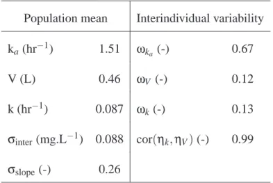
Tab. 1. Parameter estimates for the theophylline concentration dataset. A one-compartment model
was used, parameterised with the absorption rate constant ka, the volume of distribution V, and the
elimination rate constant k. A correlation between V and k (cor(ηk,ηV)) was estimated along with
the standard deviations of the three parameters. The model for the variance of the residual error is given in equation (2).
Population mean Interindividual variability
ka(hr−1) 1.51 ωka (-) 0.67
V (L) 0.46 ωV (-) 0.12
k (hr−1) 0.087 ωk(-) 0.13
σinter(mg.L−1) 0.088 cor(ηk,ηV) (-) 0.99 σslope(-) 0.26
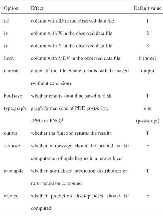
Tab. 2. Options available for the autonpde function.
Option Effect Default value
iid column with ID in the observed data file 1
ix column with X in the observed data file 2
iy column with Y in the observed data file 3
imdv column with MDV in the observed data file 0 (none)
namsav name of the file where results will be saved
(without extension)
output
boolsave whether results should be saved to disk T
type.graph graph format (one of PDF, postscript, eps
JPEG or PNG)1 (postscript)
output whether the function returns the results T
verbose whether a message should be printed as the
computation of npde begins in a new subject
F
calc.npde whether normalised prediction distribution
er-rors should be computed
T
calc.pd whether prediction discrepancies should be
computed
F
1 JPEG and PNG format are only available if the version of R used has been built to enable JPEG
and PNG output. If this is not the case, and the user selects JPEG or PNG format, the program will automatically switch to PDF and a warning will be printed.
L
EGENDS FOR FIGURES
Fig.1. Function hierarchy for the npde library, and brief description of each function. The functional
hierarchy is given for a user call to npde. With autonpde, the hierarchy is the same save for the initial
call to pdemenu.
Fig.2. Concentration versus time data for the two simulated datasets Vtrue(left) and Vfalse(right).
Fig.3. Example of a call to the functionnpde, where user input is shownin bold grey.
Fig.4. Output of the functionnpdeapplied to dataset Vtrue.
Fig.5. Graphs plotted for Vtrue. Quantile-quantile plot of npde versus the expected standard normal
distribution (upper left). Histogram of npde with the density of the standard normal distribution
overlayed (upper right). Scatterplot of npde versus observed X (lower left). Scatterplot of npde
versus ypred (lower right).
Fig.6. Output of the functionnpdeapplied to dataset Vfalse
Fig.7. Graphs plotted for Vfalse. Quantile-quantile plot of npde versus the expected standard normal
distribution (upper left). Histogram of npde with the density of the standard normal distribution
overlayed (upper right). Scatterplot of npde versus observed X (lower left). Scatterplot of npde
versus ypred (lower right).
Fig.8. Influence of the number of simulations (K) on the p-value, represented as log10(p), of the
global test under H0, for 4 simulated datasets with respectively 12, 100, 250 and 500 subjects. In each
graph, the solid line represents the median of the 10 simulations (×) performed for each value of K.
A dotted line is plotted for y=log10(0.05).
Fig.9. Influence of the number of simulations (K) on the p-value, represented as log10(p), of the
global test under H1, for 4 simulated datasets with respectively 12, 100, 250 and 500 subjects. In each
graph, the solid line represents the median of the 10 simulations (×) performed for each value of K.
A dotted line is plotted for y=log10(0.05).
Figures
Fig. 1
plot graphs save graphs to file
compute npde in one subject compute npde
read simulated data file read observed data file interactive menu
main function, called by the user
plot graphs compute pd perform tests plotnpde calcnpde graphnpde computenpde readsim readobs pdemenu npde plotnpde computepd testnpde
skewness compute skewness
compute kurtosis
kurtosis
Function hierarchy Function description
Fig. 2
0
5
10
15
20
25
0
2
4
6
8
10
Time (hr)
Concentrations (mg/L)
V
tru e0
5
10
15
20
25
0
2
4
6
8
10
Time (hr)
Concentrations (mg/L)
V
fa lseFig. 3
Name of the file containing the observed data: vtrue.dat I’m assuming file vtrue.dat has the following structure:
ID X Y ...
and does not contain a column signaling missing data. To keep, press ENTER, to change, type any letter: n
Column with ID information? 1
Column with X (eg time) information? 3 Column with Y (eg DV) information? 4
Column signaling missing data (eg MDV, press ENTER if none)? Name of the file containing the simulated data: simdata.dat
Do you want results and graphs to be saved to files (y/Y) [default=yes]? y Different formats of graphs are possible:
1. Postscript (extension eps) 2. JPEG (extension jpeg) 3. PNG (extension png)
4. Acrobat PDF (extension pdf)
Which format would you like for the graph (1-4)? 1
Name of the file (extension will be added, default=output): vtrue Do you want to compute npde (y/Y) [default=yes]? y
Do you want to compute pd (y/Y) [default=no]? y
Do you want a message printed as the computation of npde begins in a new subject (y/Y) [default=no]? n
Do you want the function to return an object (y/Y) [default=yes]? y
Fig. 4
Computing npde
Saving graphs in file vtrue.eps ---Distribution of npde: mean= -0.09442 (SE= 0.092) variance= 1.006 (SE= 0.13) skewness= -0.1048 kurtosis= -0.1783 ---Statistical tests
Wilcoxon signed rank test : 0.35 Fisher variance test : 0.931 SW test of normality : 0.839 Global adjusted p-value : 1
--Signif. codes: ’***’ 0.001 ’**’ 0.01 ’*’ 0.05 ’.’ 0.1
---Saving results in file vtrue.npde Computing pd
Fig. 5 −2 −1 0 1 2 −3 −2 −1 0 1 2
Q−Q plot versus N(0,1) for npde Sample quantiles (npde)
Theoretical Quantiles npde Frequency −3 −2 −1 0 1 2 0 5 10 15 20 0 5 10 15 20 25 −3 −2 −1 0 1 2 X npde 2 4 6 8 10 −3 −2 −1 0 1 2 Predicted Y npde
Fig. 6
Computing npde
Saving graphs in file vfalse.eps ---Distribution of npde: mean= -0.4525 (SE= 0.12 ) variance= 1.748 (SE= 0.23 ) skewness= 0.3359 kurtosis= -0.4629 ---Statistical tests
Wilcoxon signed rank test : 0.000285 *** Fisher variance test : 1.65e-06 *** SW test of normality : 0.141
Global adjusted p-value : 4.96e-06 ***
--Signif. codes: ’***’ 0.001 ’**’ 0.01 ’*’ 0.05 ’.’ 0.1
---Computing pd
Saving results in file vfalse.npde
Fig. 7 −2 −1 0 1 2 −3 −2 −1 0 1 2 3
Q−Q plot versus N(0,1) for npde Sample quantiles (npde)
Theoretical Quantiles npde Frequency −3 −2 −1 0 1 2 3 0 5 10 15 20 0 5 10 15 20 25 −3 −2 −1 0 1 2 3 X npde 2 4 6 8 10 −3 −2 −1 0 1 2 3 Predicted Y npde
Fig. 8 0 1000 2000 3000 4000 5000 −15 −10 −5 0 12 subjects K log 10 (p) −1.3 0 1000 2000 3000 4000 5000 −15 −10 −5 0 100 subjects K log 10 (p) −1.3 0 1000 2000 3000 4000 5000 −15 −10 −5 0 250 subjects K log 10 (p) −1.3 0 1000 2000 3000 4000 5000 −15 −10 −5 0 500 subjects K log 10 (p) −1.3
Fig. 9 0 1000 2000 3000 4000 5000 −150 −100 −50 0 12 subjects K log 10 (p) −1.3 0 1000 2000 3000 4000 5000 −150 −100 −50 0 100 subjects K log 10 (p) −1.3 0 1000 2000 3000 4000 5000 −150 −100 −50 0 250 subjects K log 10 (p) −1.3 0 1000 2000 3000 4000 5000 −150 −100 −50 0 500 subjects K log 10 (p) −1.3