TransCom N<sub>2</sub>O model inter-comparison – Part 1: Assessing the influence of transport and surface fluxes on tropospheric N<sub>2</sub>O variability

HAL Id: hal-03213045

https://hal.archives-ouvertes.fr/hal-03213045

Submitted on 30 Apr 2021

HAL is a multi-disciplinary open access

archive for the deposit and dissemination of

sci-entific research documents, whether they are

pub-lished or not. The documents may come from

teaching and research institutions in France or

abroad, or from public or private research centers.

L’archive ouverte pluridisciplinaire HAL, est

destinée au dépôt et à la diffusion de documents

scientifiques de niveau recherche, publiés ou non,

émanant des établissements d’enseignement et de

recherche français ou étrangers, des laboratoires

publics ou privés.

– Part 1: Assessing the influence of transport and

surface fluxes on tropospheric N₂O

variability

R. Thompson, P. Patra, K. Ishijima, E. Saikawa, M. Corazza, U. Karstens, C.

Wilson, P. Bergamaschi, E. Dlugokencky, C. Sweeney, et al.

To cite this version:

R. Thompson, P. Patra, K. Ishijima, E. Saikawa, M. Corazza, et al.. TransCom N₂O

model inter-comparison – Part 1: Assessing the influence of transport and surface fluxes on

tropo-spheric N₂O variability. Atmotropo-spheric Chemistry and Physics, European Geosciences

Union, 2014, 14 (8), pp.4349-4368. �10.5194/acp-14-4349-2014�. �hal-03213045�

www.atmos-chem-phys.net/14/4349/2014/ doi:10.5194/acp-14-4349-2014

© Author(s) 2014. CC Attribution 3.0 License.

Atmospheric

Chemistry

and Physics

TransCom N

2

O model inter-comparison – Part 1: Assessing the

influence of transport and surface fluxes on tropospheric

N

2

O variability

R. L. Thompson1,2, P. K. Patra3, K. Ishijima3, E. Saikawa4,5, M. Corazza6, U. Karstens7, C. Wilson8,9, P. Bergamaschi6, E. Dlugokencky9, C. Sweeney9, R. G. Prinn4, R. F. Weiss10, S. O’Doherty11, P. J. Fraser12, L. P. Steele12, P. B. Krummel12, M. Saunois2, M. Chipperfield8, and P. Bousquet2

1_{Norwegian Institute for Air Research, Kjeller, Norway}

2_{Laboratoire des Sciences du Climat et l’Environnement, Gif sur Yvette, France} 3_{Research Institute for Global Change, JAMSTEC, Yokohama, Japan}

4_{Center for Global Change Science, MIT, Cambridge, MA, USA} 5_{Department of Environmental Studies, Emory University, GA, USA}

6_{Institute for Environment and Sustainability, Joint Research Centre, European Commission, Ispra, Italy} 7_{Max Planck Institute for Biogeochemistry, Jena, Germany}

8_{School of Earth and Environment, University of Leeds, Leeds, UK}

9_{NOAA Earth System Research Laboratory, Global Monitoring Division, Boulder, CO, USA} 10_{Scripps Institution of Oceanography, La Jolla, CA, USA}

11_{Atmospheric Chemistry Research Group, School of Chemistry, University of Bristol, Bristol, UK}

12_{Centre for Australian Weather and Climate Research, CSIRO, Marine and Atmospheric Research, Aspendale,}

Victoria, Australia

Correspondence to: R. Thompson (rona.thompson@nilu.no)

Received: 15 November 2013 – Published in Atmos. Chem. Phys. Discuss.: 24 January 2014 Revised: 31 March 2014 – Accepted: 3 April 2014 – Published: 30 April 2014

Abstract. We present a comparison of chemistry-transport

models (TransCom-N2O) to examine the importance of

at-mospheric transport and surface fluxes on the variability of N2O mixing ratios in the troposphere. Six different models

and two model variants participated in the inter-comparison and simulations were made for the period 2006 to 2009. In addition to N2O, simulations of CFC-12 and SF6 were

made by a subset of four of the models to provide informa-tion on the models’ proficiency in stratosphere–troposphere exchange (STE) and meridional transport, respectively. The same prior emissions were used by all models to restrict dif-ferences among models to transport and chemistry alone. Four different N2O flux scenarios totalling between 14 and

17 TgN yr−1 (for 2005) globally were also compared. The modelled N2O mixing ratios were assessed against

observa-tions from in situ staobserva-tions, discrete air sampling networks and aircraft. All models adequately captured the large-scale

pat-terns of N2O and the vertical gradient from the troposphere

to the stratosphere and most models also adequately captured the N2O tropospheric growth rate. However, all models

un-derestimated the inter-hemispheric N2O gradient by at least

0.33 parts per billion (ppb), equivalent to 1.5 TgN, which, even after accounting for an overestimate of emissions in the Southern Ocean of circa 1.0 TgN, points to a likely underes-timate of the Northern Hemisphere source by up to 0.5 TgN and/or an overestimate of STE in the Northern Hemisphere. Comparison with aircraft data reveal that the models over-estimate the amplitude of the N2O seasonal cycle at Hawaii

(21◦_{N, 158}◦_{W) below circa 6000 m, suggesting an}

overesti-mate of the importance of stratosphere to troposphere trans-port in the lower troposphere at this latitude. In the North-ern Hemisphere, most of the models that provided CFC-12 simulations captured the phase of the CFC-12, seasonal cy-cle, indicating a reasonable representation of the timing of

STE. However, for N2O all models simulated a too early

minimum by 2 to 3 months owing to errors in the seasonal cycle in the prior soil emissions, which was not adequately represented by the terrestrial biosphere model. In the South-ern Hemisphere, most models failed to capture the N2O and

CFC-12 seasonality at Cape Grim, Tasmania, and all failed at the South Pole, whereas for SF6, all models could capture the

seasonality at all sites, suggesting that there are large errors in modelled vertical transport in high southern latitudes.

1 Introduction

Nitrous oxide (N2O) mixing ratios have been increasing

steadily in the atmosphere over the past few decades at an average rate of approximately 0.3 % per year, reaching 323 nmol mol−1_{(equivalently parts per billion, ppb) in recent}

years (WMO, 2011) compared with circa 270 ppb before the industrial revolution (Forster et al., 2007). The growth rate of N2O is a direct consequence of the imbalance between the

emission and the sink of N2O. The sink, that is, photolysis

and oxidation by O(1D) in the stratosphere, is thought to have increased at a slower rate than that of the emissions, which have been increasing since the mid-19th century largely due to human activities. N2O emissions are strongly tied to the

amount of reactive nitrogen (ammonium, nitrate and organic forms) in the environment. The global demand for food, and more recently bio-fuels, has led to an increasing production of reactive nitrogen, used in fertilizers, especially in the lat-ter half of the 20th century (Galloway et al., 2008). The in-crease in N2O is a major concern because it is a greenhouse

gas (GHG) and has the third largest contribution to anthro-pogenic radiative forcing after CO2and CH4(Butler, 2011).

Additionally, N2O plays an important role in stratospheric

ozone loss and the ozone-depleting-potential weighted emis-sions of N2O are now thought to be the largest of all ozone

depleting substances (Ravishankara et al., 2009).

Despite the importance of N2O, there are still many

ques-tions concerning the causes of its seasonal and, especially, inter-annual variability in the atmosphere and there are still large uncertainties in its emission. Understanding of the sea-sonal variability of N2O has improved in recent years with

the recognition of the importance of seasonal stratosphere– troposphere exchange (STE) of air masses on the tropo-spheric seasonal cycle observed at a number of sites (Nevison et al., 2007, 2011). However, there is still some debate about the additional contribution of surface fluxes and lateral trans-port to the seasonal cycle and the latitudinal dependence of this (Ishijima et al., 2010). Similarly, inter-annual variability in STE has been suggested to be an important determinant of inter-annual variability in tropospheric N2O (Nevison et al.,

2011); however, recent studies point to a greater importance of tropospheric transport and variations in surface emissions (Saikawa et al., 2013; Thompson et al., 2013, 2014a).

N2O emissions can be estimated from atmospheric

obser-vations with the use of an atmospheric chemistry transport model (CTM) to translate between concentrations and fluxes. This is formalized in atmospheric inversions, where the esti-mated fluxes are those that provide the best fit to the observa-tions while remaining within the bounds of the prior flux esti-mate and the assigned uncertainties. However, extracting in-formation about N2O fluxes from atmospheric observations

is extremely challenging owing to the small signal-to-noise ratio of these measurements. For instance, the typical preci-sion on a discrete air sample is about 0.3 ppb while the an-nual mean inter-hemispheric gradient is 1.4 ppb. In addition, there are complications of atmospheric transport, in particu-lar, STE (Nevison et al., 2011). This is one of the main mo-tivations for this study, i.e. to investigate what can be learnt from atmospheric measurements of N2O and to what extent

these can advance knowledge about surface fluxes. Simu-lations of N2O using CTMs can help our understanding of

the influence of transport on N2O spatial and temporal

vari-ability. Ultimately though, our knowledge about N2O

emis-sions through atmospheric inveremis-sions will only improve with a quantification of the uncertainties in modelled atmospheric transport and in the prior emissions.

TransCom is a community that was established in the early 1990s primarily to examine the performance of CTMs. Early studies included verification of transport using the anthro-pogenic tracer SF6 (Denning et al., 1999) and examining

simulations of atmospheric CO2 (Law et al., 1996; Law et

al., 2008). More recently, there was a TransCom study to in-vestigate the roles of emissions, transport and chemical loss on CH4(Patra et al., 2011). In this TransCom study, we

ex-amine the influence of emissions, tropospheric transport and STE on the variability in atmospheric N2O. In particular,

we focus on annual to seasonal timescales. Additionally, we aim to assess the influence of atmospheric transport errors on modelled N2O concentrations, which are used in the

in-terpretation of inverse modelling results for N2O emissions

(discussed in a companion paper: Thompson et al. 2014b). Six different models and two model variants are included in this forward inter-comparison study and five atmospheric in-version models are included in the inin-version study.

In Sect. 2, we describe the atmospheric observations used in the inter-comparison and give details about the models that participated in this study as well as about the study’s protocol. Following this, in Sect. 3.1, we present the comparison of large-scale transport features such as the inter-hemispheric (IH) gradient and cross-tropopause gradient. In Sect. 3.2, we examine the tropospheric N2O seasonal cycle

and use comparisons with SF6and CFC-12 to help

disentan-gle the contributions from STE, tropospheric transport and surface emissions on N2O concentrations. CFC-12 has been

previously used as a tracer for STE (Nevison et al., 2007) as it has comparatively well-known emissions, which have little seasonal variability but, like N2O, it is only lost in the

Table 1. Transport model overview.

Model Institution Resolution Meteorology Max Alt. Horizontal Vertical (hPa)

(lon × lat)

MOZART41 MIT/Emory 2.5◦×1.88◦ 56 σ8 MERRA10 2 offline ACTMt42l322 RIGC 2.8◦×2.8◦ 32 σ NCEP211 3 online ACTMt42l673 RIGC 2.8◦×2.8◦ 67 σ JRA2512 0.01 online TM54 JRC 6.0◦×4.0◦ 25 η9 ERA-Interim13 0.5 offline TM3-NCEP5 MPI-BGC 5.0◦×3.75◦ 19 η NCEP 23 offline TM3-ERA5 MPI-BGC 5.0◦×3.75◦ 26 η ERA-Interim 1 offline LMDZ46 LMD/LSCE 3.75◦×2.5◦ 19 η ERA-Interim 4 online TOMCAT7 Univ. of Leeds 2.8◦×2.8◦ 60 η ERA-Interim 0.1 offline

1_{Emmons et al. (2010).} 2_{Patra et al. (2009).} 3_{Ishijima et al. (2010).} 4_{Corazza et al. (2011).} 5_{Heimann and Körner (2003).} 6_{Hourdin et al. (2006).} 7_{Chipperfield (2006).}

8_{σrefers to the sigma terrain-following vertical coordinate system.}

9_{ηrefers to the eta coordinate system that smoothly transitions from the sigma coordinate near the surface to a pressure coordinate in}

the stratosphere.

10_{Modern ERa Retrospective Analysis for research and applications.} 11_{National Centers for Environmental Protection.}

12_{Japanese 25-year Reanalysis project.}

13_{European Centre for Medium-Range Weather Forecasting Reanalysis.}

as it also has comparatively well-known emissions, which are largely in the Northern Hemisphere (NH) and it can be treated as inert since it has an estimated lifetime of between 800 and 3200 years (Morris et al., 1995; Ravishankara et al., 1993). Lastly, in Sect. 4, we discuss what can be learnt about N2O emissions from model–observation comparisons

and the implications of atmospheric transport uncertainties for N2O emission estimates from inversions.

2 Observations, models and methods 2.1 Modelling protocol

A schematic overview of the modelling protocol is shown in Fig. 1 with the different components of the model set-up. To facilitate the analysis of the results in terms of atmo-spheric transport, all modelling groups were requested to use the same prior fluxes (for N2O, SF6 and CFC-12) and the

same magnitude for the stratospheric sinks of N2O and

CFC-12. On the other hand, each transport model was used with its own meteorological analysis data or, alternatively, meteoro-logical fields nudged to analysis data in offline atmospheric transport runs (see Table 1). Since each transport model has different vertical and horizontal resolution, each model was also used with its own initial 3-D mixing ratio fields.

For simulations of N2O, it was necessary to account for the

loss of N2O in the stratosphere due to photolysis (circa 90 %

of the loss) and oxidation by O(1D) (circa 10 % of the loss) (Minschwaner et al., 1993). These processes can be

summa-rized by the following three equations: N2O hv −→N2+O1D (R1) N2O + O1D k1 −→2NO (R2) (k1=6.7 × 10−11cm3molecule−1s−1) N2O + O1D k2 −→N2+O2 (R3) (k2=4.4 × 10−11cm3molecule−1s−1)

Losses of N2O were calculated on the basis of these

equa-tions within each CTM for every grid cell and time step. Al-though the exact photolysis and oxidation rates varied be-tween models, these were scaled such that the global annual total loss of N2O was approximately 12.5 TgN, consistent

with estimates of the atmospheric abundance and the life-time of N2O, which is estimated to be between 124 and 130

years (Prather et al., 2012; Volk et al., 1997). Similarly, for models participating in the CFC-12 inter-comparison, it was necessary to account for photolysis of CFC-12 in the strato-sphere (R4), which accounts for 93 to 97 % of the total loss (Seinfeld and Pandis, 1998). This was done in the same way as for N2O – that is, the photolysis rates were scaled to be

consistent with a CFC-12 lifetime of circa 100 years:

CF2Cl2

hv

−→CFCl + Cl q (R4)

Model simulations were made using meteorology and sur-face emissions for the period from 1 January 2005 to 31 De-cember 2009, with 2005 being considered as a “spin-up” year

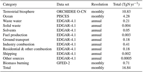
Table 2. Overview of the reference prior fluxes (OCNPIC) (totals shown for 2005).

Category Data set Resolution Total (TgN yr−1)

Terrestrial biosphere ORCHIDEE O-CN monthly 10.83

Ocean PISCES monthly 4.28

Waste water EDGAR-4.1 annual 0.21

Solid waste EDGAR-4.1 annual 0.004

Solvents EDGAR-4.1 annual 0.05

Fuel production EDGAR-4.1 annual 0.003 Ground transport EDGAR-4.1 annual 0.18 Industry combustion EDGAR-4.1 annual 0.41 Residential & other combustion EDGAR-4.1 annual 0.18

Shipping EDGAR-4.1 annual 0.002

Other sources EDGAR-4.1 annual 0.0005 Biomass burning GFED-2 monthly 0.71

Total monthly 16.84

Table 3. Overview of the additional prior fluxes (totals shown for 2005).

Flux set Categories Data set Resolution Total (TgN yr−1)

OCNN95 terrestrial biosphere ORCHIDEE OCN monthly 10.83 ocean Nevison et al. 1995 monthly 3.59 anthropogenic EDGAR-4.1a annual 1.04 biomass burning GFED-2 monthly 0.71

total 16.17

OCNN04 terrestrial biosphere ORCHIDEE OCN monthly 10.83 ocean Nevison et al. 2004 monthly 4.44 anthropogenic EDGAR-4.1 annual 1.04 biomass burning GFED-2 monthly 0.71

total 17.02

BWMN04 natural ecosystem Bouwman et al. 2002 monthly 4.59 ocean Nevison et al. 2004 monthly 4.44 anthropogenic and agriculture EDGAR-4.1b annual 4.54 biomass burning GFED-2 monthly 0.71

total 14.28

a_{EDGAR categories: 6B, 6A-6C, 3, 1B, 1A3bce, 1A2-2, 1A4-5, 1A3d, 7.} b_{EDGAR categories: 6B, 6A-6C, 3, 1B, 1A3bce, 1A2-2, 1A4-5, 1A3d, 7, 4.}

and, therefore, not included in the analysis. A 1-year spin-up was considered sufficient as all models started already with their best-estimated initial conditions taken from pre-vious model integrations.

2.2 Prior fluxes

Four different N2O emission scenarios were provided to

in-vestigate the influence of varying terrestrial and ocean fluxes. All scenarios were comprised of fluxes from the terrestrial biosphere, oceans, biomass burning, waste, fuel combustion and industry and differed only in the estimate of either the terrestrial biosphere or the ocean fluxes (see Tables 2 and 3). Each component flux used to build the scenarios is described

below (these were originally provided at monthly temporal and 1.0◦× 1.0◦spatial resolution unless otherwise stated):

1. Terrestrial biosphere: includes fluxes from natural and cultivated ecosystems from the ORCHIDEE O-CN ter-restrial biosphere model (Zaehle and Friend, 2010). The model is driven by climate data (CRU-NCEP) and inter-annually varying N inputs. Data were originally provided at 3.75◦_×2.5◦_{(longitude by latitude)}

resolu-tion. These fluxes are referred to as OCN.

2. Natural ecosystem: fluxes from uncultivated ecosys-tems from the empirical model of Bouwman et al. (2002). These fluxes are annual only and are a cli-matological mean.

Fig. 1. Schematic of the TransCom-N₂O modelling protocol.

3. Agriculture: fluxes from cultivated ecosystems from EDGAR-4.1 at annual resolution (Emission Database for Greenhouse gas and Atmospheric Research, avail-able at: http://edgar.jrc.ec.europa.eu/index.php). These fluxes together with the natural ecosystem fluxes of Bouwman et al. (2002) are referred to as BWM. 4. Waste, combustion and industry: fluxes from fossil

fuel combustion, industrial solvents, solid and water waste provided by EDGAR-4.1 at annual resolution (data available at: http://edgar.jrc.ec.europa.eu/index. php).

5. Ocean: three different flux estimates were used. The first estimate, PIC, was taken from the ocean biogeo-chemistry model, PISCES (Aumont and Bopp, 2006) with an original non-regular resolution of approxi-mately 2◦longitude × 1◦latitude. The second and third estimates were based on extrapolations of observations of N2O partial pressure anomalies in the surface ocean

that have been coupled to air–sea gas exchange coef-ficients. The N95 fluxes use the Nevison et al. (1995) estimate at 1.0◦_×1.0◦_{resolution, while the N04 fluxes}

use the Nevison et al. (2004) estimate at 0.5◦×0.5◦ resolution.

6. Biomass burning: fluxes from GFED-2.1 (Global Fire Emissions Database; van der Werf et al., 2010). The four flux estimates were then formed using one of the terrestrial biosphere fluxes, OCN or BWM, and one of the ocean fluxes, PIC, N95 or N04, plus the fluxes from biomass burning, waste, combustion and industry. The scenario, OC-NPIC, was used as the control scenario and was used for all model–observation comparisons unless otherwise stated.

Emissions of CFC-12 were provided based on the EDGAR-2 estimate but were scaled to the annual global to-tals estimated by McCulloch et al. (2003). The global emis-sion in e.g. 2006 was 40 Gg yr−1. SF6emissions were based

on the EDGAR-4.1 estimate and were scaled to the top-down global annual totals of Levin et al. (2010). The global emis-sion in 2006 was 6.3 Gg yr−1. Both CFC-12 and SF6

emis-sions were at 1.0◦×1.0◦spatial resolution and were linearly interpolated to monthly temporal resolution.

2.3 Transport models

Six models and two of their variants participated in the inter-comparison of modelled N2O mixing ratios and all of

these models have also been included in at least one pre-vious TransCom experiment (Law et al. 2008; Patra et al. 2011). The salient features of each transport model, i.e. the horizontal and vertical resolution and meteorological in-put, are given in Table 1. All models used meteorologi-cal fields from weather forecast models (MERRA, NCEP, JRA25 and ECMWF) either by interpolating (offline mod-els) or by nudging towards fields of horizontal winds and temperature (online models). Model output was generated at each site used in the analysis (see Sect. 2.4): as an hourly average (ACTMt42l32, ACTMt42l67), a 1.5-hourly average (TM5), an interpolation to the observation time step (TM3-NCEP, TM3-ERA) or at the closest model time step to the observation time (in both LMDZ4 and in TOMCAT this is 30 min). Additionally, 3-D fields of monthly mean N2O

mix-ing ratios were archived (higher temporal resolutions were not considered since this study only looks at seasonal and longer timescales and owing to the large file sizes).

2.4 Observations and data processing

Atmospheric observations of N2O dry-air mole fractions

were pooled from three global networks: NOAA CCGG (Na-tional Oceanic and Atmospheric Administration, Carbon Cy-cle and Greenhouse Gases), NOAA HATS (Halocarbons and other Atmospheric Trace Species) and AGAGE (Advanced Global Atmospheric Gases Experiment), as well as from regular aircraft transects made by NOAA (see Table 4 and Fig. S2). Discrete air samples (flasks) taken in the NOAA CCGG network and in aircraft profiles were analysed for N2O using GC-ECD (Gas Chromatography with an Electron

Capture Detector) and are reported on the NOAA-2006A cal-ibration scale (Hall et al., 2007), and have a reproducibil-ity of 0.4 ppb based on the mean difference of flask pairs. Both NOAA HATS and AGAGE operate networks of in situ GC-ECD instruments. NOAA HATS data are reported on the NOAA-2006A scale (Hall et al., 2007) and have a repro-ducibility of approximately 0.3 ppb (Thompson et al., 2004) and data from AGAGE are reported on the SIO-1998 scale and have a precision of approximately 0.1 ppb (Prinn et al., 2000). In addition, observations of CFC-12 and SF6 mole

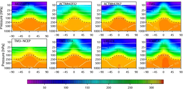
Fig. 2. Simulated zonal and annual mean latitude–altitude cross sections of N2O mixing ratio (ppb) from eight models shown for 2007.

Superimposed are contours of annual mean potential temperature (K) (white lines) and mean tropopause height (black dotted line).

fractions (pmol mol−1, equivalently parts per trillion, ppt) were used from the NOAA HATS and AGAGE networks. Both NOAA HATS measurements were made using in situ GC-ECD while AGAGE measurements of CFC-12 were made using GC-ECD and SF6 measurements were made

with GC Mass Spectrometry (GC-MS). CFC-12 data are re-ported on the NOAA-2008 (NOAA HATS) and SIO-2005 (AGAGE) scales and SF6 data are reported on the

NOAA-2006 (NOAA HATS) and SIO-2005 (AGAGE) scales. Surface measurements were filtered for outliers using an iterative filter removing values that were outside two stan-dard deviations of the mean over a time interval of 3 months for flask measurements and 3 days for in situ measurements. Data were available at approximately hourly resolution for in situ data and approximately 2-weekly resolution for flask data. For N2O, calibration offsets between networks, and

even between in situ GCs within a network, are considerable compared to the measurement precision; therefore, prior val-ues of these offsets were estimated by comparing time series from different networks and added to the observations for the model–observation comparison (see Table 5).

Mean seasonal cycles were calculated for N2O, CFC-12

and SF6 by first removing the multi-annual trend, fitted as

a second-order polynomial for N2O and SF6and as a

third-order polynomial for CFC-12, and then filtering the time se-ries for high-frequency noise using a Butterworth filter. The residuals for each month were then averaged over all years. This method was chosen preferentially over methods involv-ing fittinvolv-ing harmonic curves as these parametrizations impose a strong prior form on the seasonal cycle, which may be un-realistic at sites where the cycle has small amplitude and/or is irregular.

3 Results and Discussion

3.1 Large-scale circulation and the influence on N2O

The atmospheric distribution of N2O is characterized by a

strong cross-tropopause gradient, owing to the loss of N2O

predominantly in the upper stratosphere and STE, and a south-to-north gradient in the troposphere due to stronger emissions in the NH versus the SH. This section examines these large-scale features in the models and assesses them against observational data. In the following discussion, we refer to stratosphere to troposphere transport (STT) as the transport from the stratosphere to the troposphere, which is not to be confused with stratosphere–troposphere exchange (STE), which is a general term for exchange in both direc-tions.

3.1.1 Zonal mean vertical profile

Figure 2 shows the variation of the annual zonal mean N2O

concentration with pressure and latitude for each model us-ing the control flux estimate, OCNPIC (the general features of the zonal mean profiles do not differ from the other flux estimates and are, therefore, not shown). Generally, the large-scale features of the N2O atmospheric gradient are similar in

all simulations. However, they vary in the strength of the tro-pospheric south-to-north gradient and the gradient across the tropopause and in the stratosphere. The strength of the cross-tropopause gradient is largely determined by the rate of STE, which depends on the strength of the Brewer–Dobson circu-lation as well as on tropopause folding events, cut-off lows and small-scale mixing associated with upper-level fronts and cyclones (Holton et al., 1995). The Brewer–Dobson cir-culation oscillates seasonally with air ascending diabatically across the tropopause in the tropics, stratospheric poleward

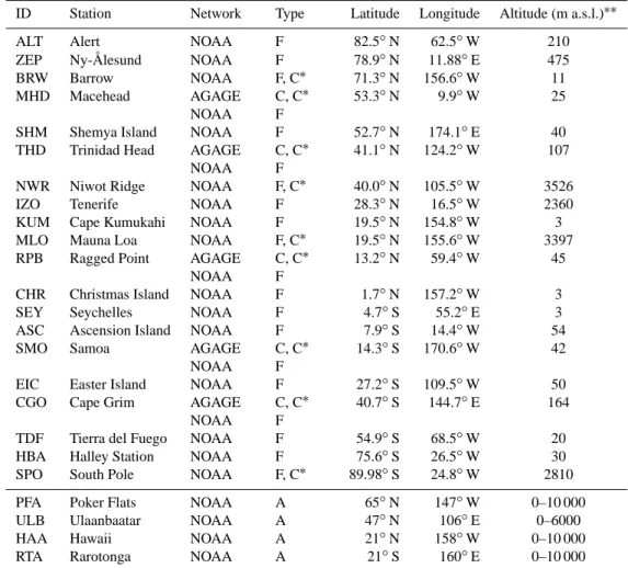
Table 4. Atmospheric sites used in the analysis.

ID Station Network Type Latitude Longitude Altitude (m a.s.l.)∗∗

ALT Alert NOAA F 82.5◦N 62.5◦W 210

ZEP Ny-Ålesund NOAA F 78.9◦N 11.88◦E 475 BRW Barrow NOAA F, C∗ 71.3◦N 156.6◦W 11 MHD Macehead AGAGE NOAA C, C∗ F 53.3◦N 9.9◦W 25 SHM Shemya Island NOAA F 52.7◦N 174.1◦E 40 THD Trinidad Head AGAGE

NOAA

C, C∗ F

41.1◦N 124.2◦W 107 NWR Niwot Ridge NOAA F, C∗ 40.0◦N 105.5◦W 3526 IZO Tenerife NOAA F 28.3◦N 16.5◦W 2360 KUM Cape Kumukahi NOAA F 19.5◦N 154.8◦W 3 MLO Mauna Loa NOAA F, C∗ 19.5◦N 155.6◦W 3397 RPB Ragged Point AGAGE

NOAA

C, C∗ F

13.2◦N 59.4◦W 45 CHR Christmas Island NOAA F 1.7◦N 157.2◦W 3 SEY Seychelles NOAA F 4.7◦S 55.2◦E 3 ASC Ascension Island NOAA F 7.9◦S 14.4◦W 54

SMO Samoa AGAGE

NOAA

C, C∗ F

14.3◦S 170.6◦W 42 EIC Easter Island NOAA F 27.2◦S 109.5◦W 50 CGO Cape Grim AGAGE

NOAA

C, C∗ F

40.7◦S 144.7◦E 164 TDF Tierra del Fuego NOAA F 54.9◦S 68.5◦W 20 HBA Halley Station NOAA F 75.6◦S 26.5◦W 30 SPO South Pole NOAA F, C∗ 89.98◦S 24.8◦W 2810 PFA Poker Flats NOAA A 65◦N 147◦W 0–10 000 ULB Ulaanbaatar NOAA A 47◦N 106◦E 0–6000 HAA Hawaii NOAA A 21◦N 158◦W 0–10 000 RTA Rarotonga NOAA A 21◦S 160◦E 0–10 000 F = flask measurement.

C = continuous (in situ) measurement.

C∗= continuous (in situ) measurement of CFC-12 and SF6.

A = aircraft flask measurement. ∗∗_{Metres above sea level.}

Table 5. Calibration offsets relative to the NOAA2006A scale. Site Mean offset (ppb)

MHD 0.25

THD −0.30

RPB 0.00

SMO 0.20

CGO 0.20

transport in the winter hemisphere, and diabatically descend-ing air across the tropopause in the high latitudes in winter (Holton et al., 1995). The seasonal influence of the Brewer– Dobson circulation on N2O mixing ratios is better resolved in

MOZART4, ACTMt42l67, TM5, TM3-ERA and TOMCAT than in the models with low vertical resolution (LMDZ4 with only 19-eta layers) and those with few stratospheric layers (ACTMt42l32 and TM3-NCEP) (see Fig. S1).

The stratosphere can be classified into an “overworld” and an “underworld” to better describe STE. The overworld lies entirely above the 380 K isentrope, while the underworld has the tropopause as its lower bound and the 380 K isen-trope as its upper bound. Isentropic surfaces intersect the tropopause in the extra-tropics, lying partly in the lower extra-tropical stratosphere and partly in the troposphere. Air masses can thus be mixed adiabatically between the tropo-sphere and lower stratotropo-sphere along isentropes that inter-sect the tropopause (Holton et al., 1995). Since on annual timescales there is no net change in the mass of the lower stratosphere, exchange across the 380 K isentropic surface can be considered as representative of the net STE (Schoe-berl, 2004). This is a particularly useful simplification when considering the budgets of species such as N2O and

CFC-12, which have a source in the troposphere and sink in the stratosphere. Table 6 shows the height of the tropopause and the gradients across the tropopause and the 380 K isentropic

Table 6. Annual mean height of the tropopause (hPa) and the N₂O gradient (ppb) across the tropopause (cross-tropopause CT) and the 380 K isentrope. Tropics are defined as between 10◦S and 10◦N and extra-tropics are defined as latitudes higher than 30◦.

Tropopause height CT gradienta Gradient across 380 Kb Tropics Extra-tropics Tropics Extra-tropics Tropics Extra-tropics

MOZART4 103 239 1.0 0.6 1.0 4.2 ACTMt42l32 105 232 0.2 1.0 0.2 3.1 ACTMt42l67 106 233 0.1 0.9 0.1 3.3 TM5 105 233 2.6 1.3 2.6 5.5 TM3-NCEP 101 234 0.5 0.3 0.5 1.5 TM3-ERA 105 236 0.6 0.4 0.6 2.6 LMDZ4 109 226 6.2 0.3 6.2 8.0 TOMCAT 102 238 0.6 1.3 0.6 3.3

a_{Normalized to a CT pressure difference of 10 hPa.}

b_{Normalized to a pressure difference across the 380 K isentrope of 10 hPa.}

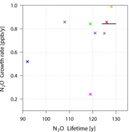
Fig. 3. Modelled and observed N2O growth rates (ppb/y)

ver-sus lifetimes (y). Legend: Mozart4, yellow; ACTMt42l32, blue; ACTMt42l67, green; TM5, grey-blue; NCEP, purple; TM3-ERA, red; LMDZ4, magenta; TOMCAT, dark green; observed (cov-ering the range of estimated lifetimes), black line.

surface in each model. Tropopause heights were calculated as the height at which the temperature lapse rate becomes less than 2 K km−1, with the added condition that the lapse rate from that height up to 2 km higher must also not exceed 2 K km−1, following the method of Reichler et al. (2003). The height of the tropopause and 380 K isentrope is fairly consistent between all models, i.e. within ± 4 % and ± 12 % of the mean, respectively. LMDZ4 has the strongest gradi-ents across 380 K isentrope in the tropics and extra-tropics owing to the low vertical resolution, while TM3-NCEP has the weakest gradients owing to strong vertical mixing.

3.1.2 Growth rate and lifetime

The tropospheric growth rate of N2O is determined by the

sum of the surface emissions and the net flux of N2O across

the tropopause and, on annual timescales, across the 380 K isentrope. Since all models use the same prior fluxes (OC-NPIC), differences in the modelled growth rates are due di-rectly to differences in the net cross-tropopause N2O flux,

which depend on the upward and downward mass fluxes and on the above- and below-tropopause N2O mixing

ra-tios, factors that are determined by the meteorological data used as well as on the vertical definition of the models. Ta-ble 7 shows the annual mean (2006–2009) tropospheric N2O

growth rates, total abundance, total sink and the atmospheric lifetime of N2O. Tropospheric growth rates were calculated

in both the models and the observations as the mean growth rate at background surface sites (these were ZEP, BRW, ALT, SHM, MHD, THD, IZO, KUM, MLO, RPB, CHR, SEY, SMO, ASC, EIC, CGO, TDF, HBA and SPO; for a descrip-tion of the sites see Table 4). The total sink was calculated directly by adding up the loss at each time step (except in ACTMt42l32 where it was calculated as the difference be-tween the total source and the change in total burden) and the lifetime was calculated as the atmospheric N2O

abun-dance up to approximately 50 hPa divided by the global an-nual loss. Most models have tropospheric growth rates close to the observed rate of 0.84 ppb yr−1with the exceptions of ACTMt42l32 and LMDZ4, which have substantially lower rates. Figure 3 shows the relationship between growth rate and lifetime for the observations and models. Although in ACTMt42l32 the low growth rate can be explained by the anomalously large sink (16 TgN yr−1)and correspondingly short lifetime (92 years), in LMDZ4 it is not so straight-forward. LMDZ4 has been shown to be a relatively dif-fuse model with fast venting of the planetary boundary layer (PBL) (Geels et al., 2007), which results in N2O being mixed

too rapidly into higher altitudes and insufficient accumula-tion of N2O in the PBL. TOMCAT, despite capturing the

growth rate, has a shorter lifetime owing to the low abun-dance of N2O in the troposphere and stratosphere. The

Table 7. Annual mean (2006–2009) tropospheric growth rate, atmospheric lifetime, atmospheric abundance (up to 50 hPa) and global total sink of N2O.

Growth rate Lifetime Abundance Sink (ppb yr−1) (years) (TgN) (TgN yr−1) Observed 0.84 124–130∗ – – MOZART4 0.99 128 1608 12.6 ACTMt42l32 0.52 92 1489 16.2 ACTMt42l67 0.84 119 1470 12.4 TM5 0.76 125 1544 12.4 TM3-NCEP 0.76 121 1515 12.5 TM3-ERA 0.86 126 1571 12.5 LMDZ4 0.24 119 1496 12.6 TOMCAT 0.86 108 1352 12.5

∗_{Independent estimates of the lifetime (Prather et al., 2012; Volk et al., 1997).}

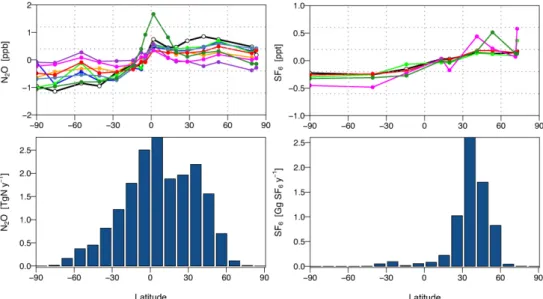
Table 8. Correlations of modelled and observed zonal mean meridional gradients for different flux scenarios (mean 2006–2009). Also shown are the inter-hemispheric differences (IHD) calculated as the mean of values for all background sites north of 20◦N minus the mean of all values for sites south of 20◦S. The observed IHD for N2O and SF6were 1.44 ppb and 0.36 ppt, respectively. R values in brackets were not

significant at the 95 % confidence level.

Model OCNPIC OCNN04 OCNN95 BWMN04 SF6

R IHD R IHD R IHD R IHD R IHD

MOZART4 0.90 0.60 – – – – – – – – ACTMt42l32 0.89 1.00 0.88 1.01 0.85 1.09 0.85 0.96 – – ACTMt42l67 0.94 1.11 0.91 1.09 0.89 1.16 0.89 0.97 0.90 0.41 TM5 0.95 1.06 0.93 1.09 0.89 1.16 0.88 0.93 – – TM3-NCEP (−0.04) −0.18 (−0.26) −0.27 (−0.27) −0.20 (−0.42) −0.31 – – TM3-ERA 0.91 0.72 0.85 0.72 0.81 0.79 0.79 0.56 0.99 0.39 LMDZ4 0.58 0.16 0.42 0.11 0.46 0.17 (0.02) −0.01 0.91 0.69 TOMCAT 0.78 0.98 0.83 0.96 0.84 0.97 0.86 0.76 0.87 0.50

to some extent by using longer spin-up times, which would bring the vertical gradients closer to steady state.

3.2 Tropospheric transport 3.2.1 Vertical gradients

Vertical mixing ratio gradients represent the combined influ-ence of surface fluxes and atmospheric transport. For N2O,

the surface fluxes are largely from the land and these are predominantly positive, therefore the mixing ratio gener-ally decreases with altitude. Sites located in the interior or downwind of continents show stronger gradients than those downwind of ocean basins owing to the stronger in-fluence of land fluxes. However, at sites where there are only weak surface fluxes, the gradient may be heavily influ-enced by lateral transport and in some cases become pos-itive in the troposphere. Figure 4 shows the seasonal and annual mean modelled (using the OCNPIC flux scenario) and observed vertical gradients of N2O mixing ratio at the

NOAA GMD aircraft profiling sites: Raratonga (RTA, 21◦S, 160◦E), Hawaii (HAA, 21◦N, 158◦W), Ulaanbaatar (ULB,

47◦N, 106◦E) and Poker Flats (PFA, 65◦N, 147◦W). For all vertical gradients (from the surface to 6000 m), the mean modelled/observed tropospheric mixing ratio at each station has been subtracted. At RTA, located in the South Pacific, a strong positive N2O gradient of approximately 0.8 ppb (0

to 6000 m) is observed in June–August, as well as in the annual mean, while no significant gradient is observed in December–February. A similar feature is also seen in the SF6

profiles at this site (not shown). The seasonal change in gradi-ent corresponds with the north–south oscillation of the inter-tropical convergence zone (ITCZ). In the NH summer the ITCZ lies north of the Equator, thus air from the NH tropics, which has a higher N2O mixing ratio, is mixed into the

south-ern Hadley cell and descends in the SH sub-tropics. Only the two CTM models and TOMCAT approximately capture the strength of the gradient but in TOMCAT, the maximum mixing ratio occurs at too low altitude. The other models (MOZART4, TM5, TM3-NCEP, TM3-ERA and LMDZ4) all underestimate the June–August and annual mean gradients to varying degrees. This appears not to be simply related to the inter-hemispheric (IH) exchange time, as TM5 has a long IH

Fig. 4. Vertical profiles of N2O (ppb) at RTA, HAA, ULB and PFA

(from top to bottom). The mean tropospheric mixing ratio at each site has been subtracted from the vertical profile. DJF = December, January, February; JJA = June, July, August; ANN = annual. Leg-end: Mozart4, yellow; ACTMt42l32, blue; ACTMt42l67, green; TM5, grey-blue; TM3-NCEP, purple; TM3-ERA, red; LMDZ4, ma-genta; TOMCAT, dark green; observed, black.

exchange time, while in LMDZ4 it is relatively short and in MOZART4 it is close to that observed (Patra et al., 2011). At HAA, located in the North Pacific, the air column above the PBL is very well mixed owing to the absence of strong local sources and to vigorous vertical mixing. All models are

able to reproduce the observed vertical profile at this site. ULB is a mid-latitude station in central Mongolia. A nega-tive vertical gradient is observed in all seasons, except au-tumn when it is positive, and has an annual mean value of approximately 0.4 ppb (from 1500 to 4000 m). The gradient is underestimated by all models (with the exception of TOM-CAT in June–August) suggesting that either the emissions are underestimated in central Asia or that the modelled vertical mixing for this region is too strong. Although we cannot rule out the first possibility, the latter is consistent with previous studies, which found a systematic overestimate of vertical mixing in the troposphere in northern mid-latitudes by CTMs (e.g. Stephens et al., 2007). At the high northern latitude site, PFA in Alaska, weak negative gradients are observed, ap-proximately 0.2 ppb (1000 to 6000 m) for the annual mean. The gradient becomes stronger in December–February above 5000 m owing to the descent of N2O-poor air from the lower

stratosphere. At this site, the shape and strength of the gradi-ent is fairly well reproduced by all models, a feature which is discussed further in Sect. 3.3.1 in relation to the N2O

sea-sonal cycle in the high northern latitudes.

3.2.2 Meridional gradients

Meridional gradients and IH differences are some of the most commonly used constraints on tropospheric transport (Gloor et al., 2007; Patra et al., 2011). Patra et al. (2011) showed that most state-of-the-art transport models agree closely in the IH gradient of SF6 (for which the emissions are fairly

well known) as well as in the IH exchange rate. This study similarly finds good agreement with the observed SF6IH

dif-ference for all models that provided SF6 simulations;

how-ever, the agreement is much poorer for N2O (Figs. 5 and 6).

Here the IH difference is calculated as the difference between the mean of all mixing ratios at background sites between 20–90◦S and 20–90◦N. All transport models underestimate the N2O IH difference, regardless of which prior flux

sce-nario is used (Table 8 and Fig. S3). The scesce-nario BWMN04 results in the lowest IH differences for all models, while dif-ferences among the “OCN” scenarios are small and not con-sistent for all models. Considering the good agreement, or in some cases even overestimate, for SF6, the poor agreement

in the IH difference for N2O is likely due to an inaccurate

distribution of emissions between the NH and SH and/or too strong STT in the NH relative to the SH. The ocean N2O

flux estimates from Nevison et al. (1995, 2004) have been shown to overestimate the net ocean–atmosphere flux in the Southern Ocean (Hirsch et al., 2006; Huang et al., 2008) but this overestimate alone is not sufficient to explain the model– observation mismatch in the IH difference. Approximately, a difference of 6.5 TgN between the NH and SH emissions is needed to explain the observed IH mixing ratio difference of 1.44 ppb. With all models underestimating the observed gradient by at least 0.33 ppb (23 %), which is equivalent to a mass of approximately 1.5 TgN, assuming the

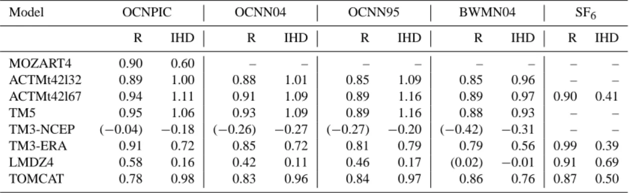
overesti-Fig. 5. Comparison of the meridional gradients of N₂O (left) and SF₆(right) using the OCNPIC scenario. Shown are the annual mean mixing ratio at background surface sites (upper panel) and the total zonal and annual prior emission estimate (lower panel). Legend: Mozart4, yellow; ACTMt42l32, blue; ACTMt42l67, green; TM5, grey-blue; TM3-NCEP, purple; TM3-ERA, red; LMDZ4, magenta; TOMCAT, dark green; observed, black.

Fig. 6. Comparisons of modelled and observed north–south gradients of N2O and SF6. N2O was simulated using the flux scenario, OCNPIC.

Gradients are calculated as the mean of values for all background sites north of 20◦N minus the mean of all values for sites south of 20◦S. The left panel shows the N2O (crosses) and SF6(circles) gradients for the observations and each model. The right panel shows the N2O

gradient versus the SF6gradient. Legend: Mozart4, yellow; ACTMt42l32, blue; ACTMt42l67, green; TM5, grey-blue; TM3-NCEP, purple;

TM3-ERA, red; LMDZ4, magenta; TOMCAT, dark green; observed, black.

mate of the Southern Ocean emissions to be approximately 1.0 TgN (Hirsch et al., 2006) leaves an unexplained north– south difference of 0.5 TgN. This could be due to errors in STT in the NH or it could be that there is still a bias in NH versus SH emissions, which could be corrected by a combi-nation of reducing SH emissions and increasing NH emis-sions. The distribution of emissions within each hemisphere also influences how well each model captures the meridional gradient. The interplay between emissions and transport

er-rors in each model explains why the models do not all re-spond in the same way to the different flux scenarios, with respect to the IH difference and meridional gradient.

3.3 Factors determining the seasonality of N2O

The seasonality of N2O is determined by a combination of

STT, tropospheric transport and surface fluxes (Ishijima et al., 2010). However, the importance of each of these determi-nants, and how this changes with latitude, remains uncertain.

Nevison et al. (2007, 2011) have demonstrated the impor-tance of seasonality in STT for the N2O seasonal cycle in

the troposphere but this mechanism appears to be less impor-tant in mid-to-low latitudes where seasonality in the surface fluxes are significant (Ishijima et al., 2010). We examine the varying influences on the tropospheric N2O seasonal cycle

focusing on seven sites, which cover a wide range of lati-tudes: BRW, MHD, THD, MLO, SMO, CGO and SPO (see Table 4). While most are background sites, MHD, CGO and THD are affected by local- to regional-scale fluxes. MHD is periodically influenced by transport from the European con-tinent (Biraud et al., 2002; Manning et al., 2011) and CGO is occasionally influenced by transport from southeastern Aus-tralia (Wilson et al., 1997). THD is affected by transport from the North American continent and, in the case of N2O, by

N2O emissions from upwelling along the Californian coast

(Lueker et al., 2003). THD is also a difficult site to model owing to the strong land/sea breeze cycle. Although this is not reproduced in global models, we expect the error in the simulated N2O due to transport to be considerably smaller

than for CO2 since there is no significant diurnal cycle in

N2O fluxes, thus there is no diurnal rectifying effect.

Only ACTMt42l67, TM3-ERA, LMDZ4 and TOMCAT participated in the CFC-12 and SF6inter-comparisons, thus

we have results for all three species from only these four models. The results of the inter-comparisons are presented in the following sections.

3.3.1 Influence of STT and tropospheric transport

To examine the influence of STT on the tropospheric sea-sonal cycle, we compare with CFC-12 because, like N2O,

the CFC-12 seasonal cycle is strongly influenced by STT (Liang et al., 2009; Nevison et al., 2007) but, unlike N2O,

the seasonality in the surface fluxes is likely to be only very small. The phase of the modelled seasonal cycle, i.e. the month of the minimum, for CFC-12 (upper panel) and N2O

(lower panel) is shown as a function of latitude and pres-sure in Fig. 7. In all models, the NH CFC-12 and N2O

min-ima appear in the lower stratosphere and upper troposphere in winter and reach the lower troposphere in May–June in the low to mid latitudes and in July–August in the high latitudes (TM3-NCEP is an exception as the minima occur about 1 month earlier compared to the other models). In the SH, the modelled minima appear in the lower stratosphere and upper troposphere in the austral spring to early summer, following the breakup of the polar vortex (except in TM3-NCEP where this is circa 2 months later). There is a lag of circa 1 to 3 months for the minima to reach the lower tro-posphere, where this occurs between January and April. We first examine the modelled seasonality in the lower tropo-sphere by comparing with observations of N2O, CFC-12 and

SF6from the AGAGE and NOAA surface networks, and

sec-ond, examine the N2O seasonality at altitude by comparing

with observations from NOAA flight profiles. Figure 8 shows

the mean seasonal cycle (2006–2009) in N2O, CFC-12 and

SF6at AGAGE and NOAA surface sites. The seasonal cycle

amplitudes have been normalized by the mean tropospheric abundance of each species to simplify the comparison be-tween them.

Northern Hemisphere

In the mid-to-high northern latitudes, a minimum in N2O and

CFC-12 is observed on average in August but for N2O the

timing varies from July to September depending on the year. At BRW and MHD, a considerable phase shift in the mod-elled N2O seasonal cycle can be seen with respect to the

ob-servations, with the modelled minimum occurring between 2 and 4 months too early (Fig. 8). For CFC-12, however, the modelled seasonality coincides with the observations at MHD and is only circa 1 month too early at BRW (one excep-tion is TM3-ERA at MHD, which has no clear seasonal cy-cle). The good agreement for CFC-12 for most models indi-cates that transport of air from the lower stratosphere into the troposphere in the high northern latitudes is adequately rep-resented and, therefore, suggests that the model–observation phase shift in N2O at these two sites is at least in part due

to incorrect seasonality in emissions in the northern mid-to-high latitudes (this will be discussed further in Sect. 3.3.2). At THD the observed and modelled seasonality in CFC-12 closely resembles that at MHD and BRW, whereas for N2O

the seasonality observed at THD has only circa half the am-plitude and the phase is quite different with respect to MHD and BRW. This points to a significant influence of N2O

sur-face fluxes on the observed seasonal cycle at this site, as also found by Nevison et al. (2011), and is most likely out of phase with the STT influence (also discussed further in Sect. 3.3.2). In the tropics, at MLO, the observed seasonal-ity in N2O and CFC-12 has the same phase but only about

a quarter of the amplitude of that seen at BRW while the modelled N2O cycle, in contrast, has approximately the same

amplitude as at BRW. The overestimate in the amplitude of the modelled seasonal cycle at MLO is most likely due to an overestimate of the influence of STT at this site (as indicated by the timing of the minimum, i.e. in May, consistent with the modelled maximum in STT and a 3-month lag from crossing the tropopause to the lower troposphere) and to the problem in the seasonality of emissions in the northern mid-to-high latitudes (see Sect. 3.3.2).

From the comparison of the observed seasonal cycles in the NH, a small shift to later CFC-12 and N2O minima with

increasing latitude was found (see Table 9) (THD is an ex-ception as the N2O seasonal cycle is strongly influenced by

local land and ocean fluxes). The shift to later minimum with increasing latitude is also reproduced by most of the models (Fig. 7) and is consistent with the current under-standing of STT. Air masses from the lower stratosphere are more strongly mixed into the troposphere in the extra-tropics

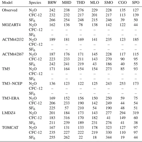
Table 9. Day of the year for the occurrence of the minimum in the mean seasonal cycle (2006–2009) of N₂O, CFC-12 and SF₆at each of the background sites.

Model Species BRW MHD THD MLO SMO CGO SPO Observed N2O 242 238 276 229 228 135 127 CFC-12 232 232 217 201 217 113 139 SF6 266 254 248 215 246 39 50 MOZART4 N₂O 162 136 78 138 142 122 44 CFC–12 – – – – – – – SF6 – – – – – – – ACTMt42l32 N2O 189 181 169 141 235 123 185 CFC–12 – – – – – – – SF6 – – – – – – – ACTMt42l67 N2O 187 176 171 145 228 117 115 CFC-12 223 233 211 143 270 90 95 SF6 242 241 219 43 186 40 55 TM5 N2O 171 164 154 154 273 85 93 CFC–12 – – – – – – – SF6 – – – – – – – TM3–NCEP N2O 136 123 122 125 243 253 173 CFC–12 – – – – – – – SF₆ – – – – – – – TM3-ERA N2O 169 152 156 150 250 59 75 CFC-12 206 233 190 142 249 44 54 SF6 225 57 210 54 190 48 51 LMDZ4 N2O 201 184 173 143 277 294 319 CFC-12 183 316 170 182 41 149 60 SF6 211 239 189 231 276 41 38 TOMCAT N2O 167 131 133 178 323 127 97 CFC-12 235 227 222 219 330 110 97 SF₆ 255 262 22 18 344 19 44

where the transport can occur adiabatically along isentropes intersecting the tropopause (James et al., 2003; Stohl et al., 2003). Furthermore, once air masses cross the tropopause, they can be rapidly transported to the lower troposphere in the downward branch of the Hadley cell around 30◦N (James et al., 2003). Therefore, the minimum is observed earlier in the mid-latitudes than in the high latitudes where the rate of vertical transport is slower. Stratospheric air masses are then transported with the mean tropospheric meridional cir-culation towards higher latitudes. Considering this, the small phase shift in modelled CFC-12 (and part of the N2O phase

shift) compared with the observations at BRW may in fact be due to too rapid transport within the troposphere rather than too rapid or too early mixing across the tropopause.

Southern Hemisphere

In SH high latitudes, the observed N2O and CFC-12 seasonal

cycles differ significantly to those of the NH (i.e. they are not 6 months out of phase). Most models predict the min-ima at SPO in January–February, i.e. too early by circa 2 months (ACTMt42l32 is an exception where the N2O

mini-mum is about 2 months too late). However, for SF6, the

mod-els match the observed cycle reasonably well at CGO and SPO. This can be understood in that the SF6 seasonal

cy-cle in the SH is largely due to seasonality in IH exchange and the strong meridional gradient in the atmosphere (Den-ning et al., 1999; Prinn et al., 2000), which is satisfactorily represented in the models. On the other hand, the N2O and

CFC-12 seasonal cycles are strongly modulated by STT and, in the case of N2O, weakly modulated by ocean fluxes. The

importance of STT has been shown previously at CGO using measurements of CFC-11 and CFC-12 (Nevison et al. 2005) and δ18O and δ15N isotopes in N2O (Park et al., 2012). The

model–observation mismatch for N2O and CFC-12 points to

a deficiency in modelling STT in the SH. However, it is not easy to explain why the maximum influence of STT (result-ing in a minimum in N2O and CFC-12) is seen in April–May,

which is 2 to 3 months later than one would expect given the winter (May to August) maximum in diabatic STT, the spring increase in tropopause height, and the spring breakup of the polar vortex, and points to gaps in our knowledge about STT in the SH. The observed seasonal cycles of N2O and

CFC-12 at SMO are closely in phase with that of SF6, which can

Fig. 7. Month of minimum in CFC-12 (upper panel) and N2O (middle and lower panel) shown for each model (the subplots) in 2007. 2 4 6 8 10 −0.4 −0.2 0.0 0.2 0.4 N2 O [ppb v] BRW 2 4 6 8 10 −0.4 −0.2 0.0 0.2 0.4MHD 2 4 6 8 10 −0.4 −0.2 0.0 0.2 0.4THD 2 4 6 8 10 −0.4 −0.2 0.0 0.2 0.4MLO 2 4 6 8 10 −0.4 −0.2 0.0 0.2 0.4SMO 2 4 6 8 10 −0.4 −0.2 0.0 0.2 0.4 CGO 2 4 6 8 10 −0.4 −0.2 0.0 0.2 0.4 SPO 2 4 6 8 10 −0.4 −0.2 0.0 0.2 0.4 CFC − 12 [pptv] 2 4 6 8 10 −0.4 −0.2 0.0 0.2 0.4 2 4 6 8 10 −0.4 −0.2 0.0 0.2 0.4 2 4 6 8 10 −0.4 −0.2 0.0 0.2 0.4 2 4 6 8 10 −0.4 −0.2 0.0 0.2 0.4 2 4 6 8 10 −0.4 −0.2 0.0 0.2 0.4 2 4 6 8 10 −0.4 −0.2 0.0 0.2 0.4 2 4 6 8 10 −2 −1 0 1 2 SF 6 [pptv] 2 4 6 8 10 −2 −1 0 1 2 2 4 6 8 10 −2 −1 0 1 2 2 4 6 8 10 −2 −1 0 1 2 2 4 6 8 10 −2 −1 0 1 2 2 4 6 8 10 −2 −1 0 1 2 2 4 6 8 10 −2 −1 0 1 2

Fig. 8. Comparison of the climatological seasonal cycles (2006–2009) of N2O (top row), CFC-12 (middle row) and SF6(bottom row) for

selected background stations (each column). Legend: Mozart4, yellow; ACTMt42l32, blue; ACTMt42l67, green; TM5, grey-blue; TM3-NCEP, purple; TM3-ERA, red; LMDZ4, magenta; TOMCAT, dark green; observed, black.

mixing ratio gradient and is consistent with previous studies (Nevison et al., 2007).

Altitude changes

To further investigate the influence of STT, we compare the modelled seasonal cycles at four different altitude ranges,

from the lower troposphere to the tropopause, with NOAA aircraft data (unfortunately there is insufficient data cover-age at RTA to be able to compare the seasonal cycles at this site). Figure 9 shows the observed and modelled N2O

as monthly means with the growth rate subtracted (as given in Table 7). At PFA, the influence of STT is seen between 6000 and 10 000 m with an observed minimum occurring

Fig. 9. Comparison of N2O at different altitudes (along the rows) at the aircraft sampling sites: PFA (left panel), ULB (middle panel; no

data were available for altitudes above 6000 m) and HAA (right panel). Data are shown as monthly means with the growth rates (as given in Table 6) subtracted. MOZART4 was adjusted with an offset of −1 ppb to fit the N2O scale. Legend: Mozart4, yellow; ACTMt42l32, blue;

ACTMt42l67, green; TM5, grey-blue; TM3-NCEP, purple; TM3-ERA, red; LMDZ4, magenta; TOMCAT, dark green; observed, black.

in late June. The timing of this minimum appears to be in-consistent with a winter maximum in diabatic STT due to the Brewer–Dobson circulation. However, as pointed out by Schoeberl (2004), most of the mass exchange between the lower stratosphere and troposphere can be related to changes in the tropopause height with the maximum mass transfer to the troposphere occurring in spring as the tropopause height is increasing – in which case, allowing for the lag time for vertical and horizontal transport within the troposphere of approximately 2 months according to Liang et al. (2009), a June minimum is not unexpected. Another consideration for the timing of the minimum is the seasonal cycle of N2O in the

stratosphere itself, which must be convolved with that of STT to explain the influence on tropospheric seasonality (Liang et al., 2009). Since N2O is destroyed photochemically,

extra-tropical stratospheric loss of N2O has a maximum in summer

and minimum in winter, thus the phase of the seasonal cycle in the stratosphere will lead to a later minimum in the tro-posphere (as compared to no seasonality in the stratosphere). Below 6000 m, the minimum occurs significantly later again, in August. The reason for the August minimum is likely twofold: (1) owing to the time needed to transport the STT influence in the mid-latitudes (where most STT occurs) to the high northern latitudes and (2) owing to the increase in PBL height, which means the fluxes are mixed into a greater

volume of air, thereby decreasing the mixing ratio. Although all models predict a too early minimum above 6000 m (by circa 2.5 months), the phase shift between the modelled and observed minima is fairly constant across all altitudes, con-sistent with the finding that the modelled vertical gradient at this site agrees with observations (see Fig. 4).

At ULB, the influence of STT can be seen between 4000 and 6000 m with a minimum in July but the amplitude of the cycle decreases at lower altitudes suggesting a weaker influence of STT in the lower troposphere at this latitude. Although the phase of the cycle in the 4000–6000 m alti-tude range is fairly closely captured by most models, they overestimate its amplitude below 4000 m. Lastly, at HAA, the observed seasonal cycle is consistent in amplitude and phase from 500 to 6000 m, owing to vigorous vertical mix-ing. However, all models predict a too early minimum below 6000 m and overestimate the amplitude suggesting that the modelled influence of STT at this latitude is too strong.

3.3.2 Influence of surface fluxes

The influence of changing the surface fluxes of N2O on the

seasonal cycle in the lower troposphere was investigated by performing four different transport model integrations with each of the four prior flux estimates: OCNPIC, OCNN95, OCNN04 and BWMN04 (see Tables 2 and 3 for details and

Fig. 10. Comparison of observed mean N2O seasonality (2006–2009) with that modelled using four different prior flux models. Each

station is shown as a separate panel and within each panel the four subplots are for each of the flux models as indicated in the top-left corner (see Tables 2 and 3 for a description of the fluxes). N2O mixing ratio is on the left axis and N2O flux (grey line) is on the right

axis. Legend: Mozart4, yellow; ACTMt42l32, blue; ACTMt42l67, green; TM5, grey-blue; TM3-NCEP, purple; TM3-ERA, red; LMDZ4, magenta; TOMCAT, dark green; observed, black.

Fig. S4 for Hovmöller plots of the flux components). Fig-ure 10 compares the observed and modelled seasonal cycles at each site (BRW, MHD, THD, MLO, SMO and CGO) as a separate panel, and the four subplots within each panel are for each of the four flux scenarios. Also shown within each subplot is the area-weighted mean N2O flux for an area

of 10◦×30◦ (latitude by longitude) centred on the site. At

BRW, the best match to the observed cycle was provided by the BWMN04 fluxes while the other three (all using OCN terrestrial biosphere fluxes) were very similar in phase and amplitude. Around the site itself, the flux is very low and there is little difference between the BWM and OCN terres-trial fluxes (the flux difference is solely due to the choice of ocean flux estimate). The improved fit to the seasonal cycle

in the mixing ratio at BRW, therefore, must result from the difference between OCN and BWM in the mid-northern lat-itudes; OCN predicts a late summer maximum while there is no seasonal cycle in BWM. The phase modelled with BWMN04 matches almost exactly (correlation coefficient

R2≥0.95) for all models except TM3-NCEP. Furthermore, considering that for CFC-12 at this site there is a phase shift of only approximately 1 month, the mismatch in the OCN simulations is unlikely to be from transport model errors. Similarly at MHD, BWMN04 provides the best fit to the observations (R2≥0.79, except TM3-NCEP). These results show that the inclusion of a seasonal cycle in the OCN ter-restrial fluxes does not improve the fit to the observations but rather makes it worse, indicating that the seasonality, in par-ticular the late summer maximum, in OCN is not realistic. From what is known about the processes driving the terres-trial biosphere N2O flux, higher emissions are expected

dur-ing the growdur-ing season owdur-ing to warmer soil temperatures leading to increased microbial activity and higher reactive nitrogen turnover rates. However, OCN most likely overesti-mates the late summer emissions while underestimating the emissions in spring and early summer. This is due to the lack of a vertically resolved soil layer, which prevents the realistic simulation of the impact of rain events and tends to predict anoxic soil conditions, necessary for N2O

pro-duction via denitrification, predominantly in summer rather than distributed throughout the year as would be more real-istic (S. Zaehle, personal communication, 2012). This result highlights the complexity of modelling terrestrial ecosystem N2O fluxes and the need for independent validation. Again at

THD, BWMN04 gives the closest fit to the observed seasonal cycle matching the amplitude but still resulting in a too early minimum by circa 3 months. Since THD is also strongly in-fluenced by N2O emissions from upwelling along the

Cali-fornian coast (Lueker et al., 2003), this model–observation mismatch may also indicate deficiencies in the coastal N2O

fluxes.

At MLO, the regional flux differences are due to differ-ences between the ocean flux models, PIC, N95 and N04. However, an improvement in the modelled seasonal cycle in N2O mixing ratio only occurs when the BWM terrestrial

fluxes are used (R2≥0.27, except TM3-NCEP, compared with no correlation with the other fluxes). This shows that the seasonality at MLO is also influenced by NH terrestrial fluxes as has also been previously shown (Patra et al., 2005). For SMO, the modelled seasonality is very similar for all flux models (N04 results in a small phase shift to a later mini-mum), which can be understood in that this site is strongly affected by IH exchange rather than the seasonality of sur-face fluxes in this latitude. In the southern mid-latitudes, at CGO, OCNPIC and OCNN95 give the best agreement to the observed seasonal cycle. Replacing the terrestrial biosphere fluxes, OCN, with BWM made no significant difference, as expected since this site is only very weakly influenced by land fluxes. For SPO, changing the fluxes had negligible

in-fluence on the modelled mixing ratios (this site is not shown), highlighting again the importance of STT at this site.

4 Summary and conclusions

This TransCom study has investigated the influence of emis-sions, tropospheric transport and stratosphere–troposphere exchange (STE) on the variability in atmospheric N2O,

fo-cusing on seasonal to annual timescales. In particular, our aim has been to examine the influence of errors in atmo-spheric transport versus errors in prior fluxes on modelled mixing ratios by comparing simulated mixing ratios with at-mospheric observations of N2O as well as CFC-12 to

as-sess the ability of models to reproduce STE and, addition-ally, of SF6to assess the tropospheric transport in the models.

Knowledge about prior flux and transport errors has impor-tant implications for the setup of inverse models for estimat-ing N2O surface emissions and for the interpretation of their

results. In total, six different transport models and two model variants were included in this inter-comparison.

To assess the representation of global-scale transport and, in particular, inter-hemispheric transport, we compared the modelled and observed IH gradients of N2O and SF6. We

found good agreement between the modelled and observed south-to-north gradient and IH difference for SF6in line with

previous studies (e.g. Patra et al., 2011), which indicates that the models adequately capture the rate of IH mixing as well as mixing between tropical and extra-tropical regions. For N2O, however, the IH difference was underestimated

com-pared to the observations in all models by at least 0.33 ppb, equivalent to approximately 1.5 TgN. Assuming that emis-sions in the Southern Ocean are overestimated by approx-imately 1.0 TgN (Hirsch et al., 2006) leaves an unexplained north–south difference of 0.5 TgN. This most likely indicates a larger NH to SH source ratio than prescribed in the prior emissions but an overestimate of the influence of STT in the NH may also still contribute to the model–observation differ-ence in the IH gradient.

Using a combination of aircraft profiles (NOAA flights) and surface sites (NOAA and AGAGE networks), we have compared the modelled and observed N2O seasonal cycles

from the surface to the upper troposphere and the CFC-12 and SF6 seasonal cycles at the surface. We found that all

models that simulated CFC-12 accurately matched the phase and amplitude of the CFC-12 cycle at MHD and were only circa 1 month out of phase at BRW. In contrast, modelled N2O seasonal cycles were all 2–3 months out of phase at

both sites. The model–observation mismatch in the N2O

sea-sonal cycle at NH sites is, thus, likely not to be due to errors in atmospheric transport, which on the basis of the CFC-12 comparison are in the order of the measurement precision (i.e. 0.1 ppb), but rather due to errors in the N2O flux.

Ad-ditionally, when the simulations using the BWM terrestrial ecosystem fluxes (as opposed to OCN) were compared, a

much better agreement with the observations was found for BRW, MHD, THD and MLO. While the BWM fluxes have no seasonal component, OCN predicts a late summer maxi-mum. Even after considering the seasonality of STT, a late summer maximum in the surface N2O fluxes in the

mid-to-high northern latitudes is inconsistent with observations. Late summer emissions are likely overestimated in OCN, while emissions in spring and autumn are likely underestimated. Furthermore, the timing of the N2O mixing ratio minimum

in the upper troposphere in the extra-tropical northern lati-tudes (in June–July) occurs too late to be predominantly due to the winter maximum in diabatic STT i.e. driven by the Brewer–Dobson circulation as previously suggested (Nevi-son et al. 2007, 2011), but rather is consistent with the effect of increasing tropopause height in spring (Schoeberl, 2004). This spring maximum in mass transfer, convoluted with the seasonality of N2O loss in the stratosphere and the lag time

for this signal to be transported in the troposphere (circa 2 months) more likely explains the phase of the observed sig-nal.

In the southern low latitudes, at SMO, the influence is mostly from IH transport as previously found for SF6

(Den-ning et al., 1999; Prinn et al., 2000) and N2O (Nevison et

al., 2007; Nevison et al., 2011), while in the SH mid-to-high latitudes, CGO and SPO are strongly influenced by STT and weakly influenced by meridional transport and ocean surface fluxes, as previously shown (Park et al., 2012). The error at these sites due to transport is significant for all models, and thus will result in errors in the seasonality and, with seasonal dependence of atmospheric transport, in the location of emis-sions estimated from atmospheric inveremis-sions.

To conclude, the comparison of modelled and observed N2O mixing ratios has been shown to provide important

constraints on the broad spatial distribution of N2O

emis-sions and, in the NH, on their seasonality. However, mod-elled N2O mixing ratios are sensitive to non-random model

transport errors, particularly in the magnitude of STT, which will contribute to errors in N2O emissions estimates from

at-mospheric inversions. In the SH mid-to-high latitudes, the influence of transport errors on modelled N2O mixing ratios

is even more important, again largely due to errors in STT, and means that current estimates of seasonality and, to some extent, the location of N2O emissions in the SH from

atmo-spheric inversions may not be reliable.

Supplementary material related to this article is available online at http://www.atmos-chem-phys.net/14/ 4349/2014/acp-14-4349-2014-supplement.pdf.

Acknowledgements. We would like to thank C. Nevison, S. Zaehle,

L. Bouwman, L. Bopp and G. van der Werf for providing their N2O

emissions estimates. We also thank F. Chevallier and S. Zaehle for their comments, which improved this article. Additionally, we would like to acknowledge everyone who contributed to the

measurements of N₂O without which we would not have been able to make this inter-comparison study.

Edited by: W. Lahoz

References

Aumont, O. and Bopp, L.: Globalizing results from ocean in situ iron fertilization studies, Global Biogeochem. Cy., 20, GB2017, doi:10.1029/2005GB002591, 2006.

Biraud, S., Ciais, P., Ramonet, M., Simmonds, P., Kazan, V., Mon-fray, P., O’Doherty, S., Spain, G., and Jennings, S. G.: Quantifi-cation of carbon dioxide, methane, nitrous oxide and chloroform emissions over Ireland from atmospheric observations at Mace Head, Tellus, 54B, 41–60, 2002.

Bouwman, A. F., Boumans, L. J. M., and Batjes, N. H.: Modeling global annual N2O and NO emissions from

fertilized fields, Global Biogeochem. Cy., 16, 1080, doi:10.1029/2001GB001812, 2002.

Butler, J. H.: The NOAA Annual Greenhouse Gas Index, from http: //www.esrl.noaa.gov/gmd/aggi/ (last access: April 2014), 2011. Chipperfield, M. P.: New version of the TOMCAT/SLIMCAT

off-line chemical transport model: Intercomparison of stratospheric tracer experiments, Q. J. Roy. Meteorol. Soc., 132, 1179–1203, 2006.

Corazza, M., Bergamaschi, P., Vermeulen, A. T., Aalto, T., Haszpra, L., Meinhardt, F., O’Doherty, S., Thompson, R., Moncrieff, J., Popa, E., Steinbacher, M., Jordan, A., Dlugokencky, E., Brühl, C., Krol, M. and Dentener, F.: Inverse modelling of European N2O emissions: assimilating observations from different

net-works, Atmos. Chem. Phys., 11, 2381–2398, doi:10.5194/acp-11-2381-2011, 2011.

Denning, A. S., Holzer, M., Gurney, K. R., Heimann, M., Law, R. M., Rayner, P. J., Fung, I. Y., Fan, S.-M., Taguchi, S., Freidling-stein, P., Balkanski, Y., Taylor, J., Maiss, M., and Levin, I.: Three-dimensional transport and concentration of SF6: A model

inter-comparison study (TransCom 2), Tellus, 51B, 266–297, 1999. Emmons, L. K., Walters, S., Hess, P. G., Lamarque, J.-F., Pfister,

G. G., Fillmore, D., Granier, C., Guenther, A., Kinnison, D., Laepple, T., Orlando, J., Tie, X., Tyndall, G., Wiedinmyer, C., Baughcum, S. L. and Kloster, S.: Description and evaluation of the Model for Ozone and Related chemical Tracers, version 4 (MOZART-4), Geosci. Model Dev., 3, 43–67, doi:10.5194/gmd-3-43-2010, 2010.

Forster, P., Ramaswamy, V., Artaxo, P., Berntsen, T., Betts, R., Fa-hey, D. W., Haywood, J., Lean, J., Lowe, D. C., Myhre, G., Nganga, J., Prinn, R., Raga, G., Schultz, M., and Van Dorland, R.: Changes in Atmospheric Constituents and in Radiative Forc-ing, Climate Change 2007: The Physical Science Basis. Contri-bution of Working Group I to the Fourth Assessment Report of the Intergovernmental Panel on Climate Change. Solomon, S., Qin, D., Manning, M., Chen, Z., Marquis, M., Averyt, K. B., Tignor, M., and Miller, H. L., Cambridge University Press, Cam-bridge, UK, 129–234, 2007.

Galloway, J. N., Townsend, A. R., Erisman, J. W., Bekunda, M., Cai, Z., Freney, J. R., Martinelli, L. A., Seitzinger, S. P., and Sutton, M. A.: Transformation of the Nitrogen Cycle: Recent Trends, Questions, and Potential Solutions, Science, 320, 889–892, 2008.