HAL Id: hal-02437458
https://hal.archives-ouvertes.fr/hal-02437458
Submitted on 13 Jan 2020HAL is a multi-disciplinary open access archive for the deposit and dissemination of sci-entific research documents, whether they are pub-lished or not. The documents may come from teaching and research institutions in France or abroad, or from public or private research centers.
L’archive ouverte pluridisciplinaire HAL, est destinée au dépôt et à la diffusion de documents scientifiques de niveau recherche, publiés ou non, émanant des établissements d’enseignement et de recherche français ou étrangers, des laboratoires publics ou privés.
Correction strategy for diffusion-weighted images
corrupted with motion: application to the DTI
evaluation of infants’ white matter
Jessica Dubois, Sofya Kulikova, Lucie Hertz-Pannier, Jean-François Mangin,
Ghislaine Dehaene-Lambertz, Cyril Poupon
To cite this version:
Jessica Dubois, Sofya Kulikova, Lucie Hertz-Pannier, Jean-François Mangin, Ghislaine Dehaene-Lambertz, et al.. Correction strategy for diffusion-weighted images corrupted with motion: application to the DTI evaluation of infants’ white matter. Magnetic Resonance Imaging, Elsevier, 2014, 32 (8), pp.981-992. �10.1016/j.mri.2014.05.007�. �hal-02437458�
Correction strategy for diffusion-weighted images corrupted with motion:
Application to the DTI evaluation of infants’ white matter
Jessica Dubois PhD 1, Sofya Kulikova2, Lucie Hertz-Pannier MD-PhD 2,
Jean-François Mangin PhD 3, Ghislaine Dehaene-Lambertz MD-PhD 1, Cyril Poupon PhD 4
Affiliations:
1: INSERM, U992, Cognitive Neuroimaging Unit, Gif-sur-Yvette, France; CEA, NeuroSpin Center, UNICOG, Gif-sur-Yvette, France; University Paris Sud, Orsay, France
2: CEA, NeuroSpin Center, UNIACT, Gif-sur-Yvette, France; INSERM, U663, Paris, France; University Paris Descartes, Paris, France
3: CEA, NeuroSpin Center, UNATI, Gif-sur-Yvette, France; University Paris Sud, Orsay, France 4: CEA, NeuroSpin Center, UNIRS, Gif-sur-Yvette, France; University Paris Sud, Orsay, France
Corresponding author:
Jessica Dubois, PhD
CEA/SAC/DSV/I2BM/NeuroSpin/Cognitive Neuroimaging Unit U992 Bât 145, point courrier 156
91191 Gif-sur-Yvette, France
Email: jessica.dubois@centraliens.net
Magnetic Resonance Imaging 2014. 32:981-992
Abstract
Objective: Diffusion imaging techniques such as DTI and HARDI are difficult to implement in
infants because of their sensitivity to subject motion. A short acquisition time is generally preferred, at the expense of spatial resolution and signal-to-noise ratio. Before estimating the local diffusion model, most pre-processing techniques only register diffusion-weighted volumes, without correcting for intra-slice artifacts due to motion or technical problems. Here, we propose a fully automated strategy, which takes advantage of a high orientation number and is based on spherical-harmonics decomposition of the diffusion signal.
Material and methods: The correction strategy is based on two successive steps: 1) automated
detection and resampling of corrupted slices; 2) correction for eddy current distortions and realignment of misregistered volumes. It was tested on DTI data from adults and non-sedated healthy infants.
Results: The methodology was validated through simulated motions applied to an uncorrupted
dataset and through comparisons with an unmoved reference. Second, we showed that the correction applied to an infant group enabled to improve DTI maps and to increase the reliability of DTI quantification in the immature cortico-spinal tract.
Conclusion: This automated strategy performed reliably on DTI datasets and can be applied to
spherical single- and multiple-shell diffusion imaging.
Keywords
I.
Introduction
Imaging the diffusion of water molecules by MRI enables the non-invasive exploration of the tissues microstructure. This is done by making the MR signal sensitive to spin motion through the application of diffusion gradients during acquisition [1]. To explore the anisotropic structure of tissues, such as the fiber organization of white matter, diffusion-weighted (DW) images are currently acquired along several orientations of the diffusion gradients taken on a single shell in the Q-space, for a fixed b-value, with models like Diffusion Tensor Imaging (DTI) and High Angular Resolution Diffusion Imaging (HARDI). In DTI, MR measurements are performed along at least 6 orientations of the diffusion gradients. In comparison with data averaging, increasing the number of orientations also improves the signal-to-noise ratio (SNR) of the resulting diffusion maps. On condition that orientations are uniformly distributed over the space [2, 3], it further enables a more precise spatial and angular estimation of the diffusion model, thus improving the local estimation of the spatial organization of tissues. But it also increases the acquisition time and thus the risk of motion artifacts. Increasing the b-value improves the reliability of diffusion models, but decreases the SNR. HARDI models, such as Q-ball imaging (QBI), better explore the tissue microstructure and anisotropy, but the acquisition of a high number of diffusion gradient orientations is required. Therefore, a compromise between image quality and acquisition time must be found.
Diffusion techniques are based on 2-dimensional (2D) acquisitions with echo planar imaging (EPI), and slices are generally acquired in an interleaved order. Because of diffusion gradients, the acquisition time of a slice is of the order of 200ms, which corresponds to a 10s scan duration to cover the whole brain with 50 slices. If for instance 30 different orientations of the diffusion gradients are acquired, the total acquisition time is at least 5 minutes (plus the acquisition time for b=0 images and calibration scans required for parallel imaging). Consequently, motion can occur during the acquisition of a slice (“intra-slice” motion) or a volume (“intra-volume” motion), or between the acquisitions corresponding to different orientations of diffusion sensitization (“inter-volume” motion). It results in two kinds of motion-related errors: 1) artifacts within a volume (signal irregularities and potential outliers with near-complete signal dropout that generate “black stripes” artifacts along the slice direction, when images are viewed from the side, or signal loss in a region of the brain, due to repeated excitation of spins during slice selection); and 2) 3D misregistration between the volumes acquired before and after the movement. Other artifacts are also frequently observed in DW images, independently of subject’s motion, because of hardware problems during acquisition like mechanical vibrations [4] or spike noise [5]. The impact of such corrupted data on DTI and QBI metrics has recently been highlighted with simulations [6].
MR diffusion techniques are particularly informative to explore the developing brain [7, 8], but they are challenging in non-sedated infants [9, 10] because of their sensitivity to subject’s motion. To improve data quality, the first step is to optimize data acquisition. Short acquisition times, relying on low orientation number, are generally used, but at the expense of accuracy. DWI and DTI sequences performed within a breath-hold of the mother have been devised for fetal brain imaging [11]. Continuous scanning has also been performed in order to acquire repeated series, whose volumes have to be registered a posteriori [12]. Alternatively, DTI acquisitions may be adapted in real time according to patient motion, by continuously adjusting all applied gradients to compensate for changes in head position [13], by identifying corrupted data according to the position and the magnitude of the largest echo-peak in the k-space [14], or by directly evaluating the quality of DTI maps, which are estimated on-line [15]. The
implementation of a self-navigation scheme with variable density spiral acquisition gradients has also enabled to remove both eddy current distortions and motion artifacts in the adult brain [16]. To deal with mechanical vibrations, Gallichan and colleagues [4] recommended a full Fourier k-space sampling, but this increases the minimum echo time and decreases the slice number available per repetition time. In infants, specific spatial distributions of diffusion orientations, which take into account their temporal order during acquisition, have enabled to reliably estimate the diffusion tensor even if the acquisition is interrupted due to motion [3, 17].
Another direction to deal with motion in DW images is to apply post-processing correction strategies, which definitely help improve the precision and accuracy of the metrics estimation in DTI [18] and HARDI imaging [19]. The most common registration technique corrects for eddy current distortions and 3D motion [20], and is based on mutual information between diffusion orientation volumes and a reference volume, with a subsequent rotation of the B-matrix before analysis of DW images [20, 21]. Integrating motion in the signal model used for the tensor estimation seems to perform superiorly compared with the conventional method [22]. In pediatric patients, an automated reconstruction software has recently been implemented [10], but it requires a dedicated acquisition for Nyquist ghost calibration and parallel imaging GRAPPA weight. These post-processing strategies hardly correct for within-slice artifacts, which are frequently observed in rapidly moving subjects like infants or due to mechanical vibrations or spike noise. The easiest solution to deal with these artifacts is to exclude the whole corrupted volumes on a simple visual basis, but it is time consuming, dependent on the experimenter and it also potentially removes uncorrupted slices. Automatic detection of outliers has previously been performed through linear correlation coefficients between DW volumes [10], during a robust estimation of the diffusion tensor [23], or by finding the local maxima on the Laplacian of DW signals across diffusion orientations [24]. For the correction of detected outliers, methods include removing such voxels [23] or volumes [10], fitting the signal using linear regression methods [4], or interpolating the Q-space signal directly on the spherical shell [6]. Recently, an algorithm which detects and removes outliers prior to 3D resampling, while taking misalignment into account, has been proposed [9]. Despite their respective advantages, all these approaches also present some drawbacks: rejecting instead of correcting the corrupted data, making hypothesis on the diffusion model, etc.
Alternatively we here propose a global post-processing methodology for automatically correcting all motion-related artifacts in DW images before computing the diffusion model. It is based on two successive steps: 1) automated detection and 2D resampling of slices corrupted by motion or technical problems (mechanical vibrations, spike noise); 2) 3D realignment of orientation volumes misregistered due to inter-volume motion and distortions stemming from eddy current. This correction strategy was applied on DTI data from 20 non-sedated infants, aged from 6 to 22 weeks. First, the two steps of the methodology were validated by simulating motion in an uncorrupted dataset. Second, we applied this strategy to all infants, and we studied quantitatively the immature cortico-spinal tract, because its development has already been detailed over this age range.
II.
Materials and methods
1. Description of the correction method
Our post-processing strategy takes advantage of a high diffusion orientation number to correct for corrupted (also called outlier) images. It relies on two successive steps: 2D resampling of the outlier individual slices, followed by 3D registration and correction of the eddy current
distortions in the resulting volumes (Figure 1). It is implemented within BrainVISA [25] in the Connectomist toolbox [26].
a. Detection of outlier slices
To detect corrupted slices, the basic concept is to compare the DW image for the ith orientation Oi to all the other orientations (Oj, j≠i), for each slice independently. To do so, the b=0 image is used as a reference and a distance between it and each DW Oi image is computed. The mutual information (MI) coefficient [27, 28] was chosen because it does not impose any particular relationship between images (except sharing some information), which makes the measurement independent of the grey level intensity that is variable across diffusion orientations, and it is a reliable and robust criterion to compare b=0 and DW images and correct eddy current distortions [29]. The outlier detection in a given slice s is done with a simple criterion: slice s for the orientation Oi is considered as an outlier if its MI coefficient is not in the range: Mean ± f x StdDev, where the mean and standard-deviation (StdDev) of MI coefficients are computed over all orientations (the median values were systematically computed and found almost equal to the means). The f factor is the only parameter to be tuned once for a specific protocol (see below). This strategy for outliers detection is fully automatic. Note that several DW images (for different orientations Oi) may be corrupted in the same slice. On the other hand, several slices may be corrupted at the same diffusion orientation, which may reveal a weakness of the gradient power amplifier or a vibration problem, in the absence of motion.
b. Resampling strategy of outlier slices
When an outlier is detected using the previous criterion, our strategy consists of resampling it instead of discarding the corresponding diffusion orientation from the set of available DW data. Corrections are performed through resampling from the non-outlier DW images in the Q-space. A decomposition of the DW signal is performed over the non-corrupted orientations, by using the modified spherical harmonics basis (SH) proposed by Frank [30]: for acquisitions performed on a single shell q, the signal of each voxel can be decomposed on this basis
( )
=
j j u j q SH S u q S 0 ( , ) ( ) , where u represents a normed vector coding for the diffusion orientation. This decomposition is limited to the 6th order to avoid overfitting, and some regularization is introduced by Descoteaux and colleagues to improve its reliability [31]. The resulting SH coefficients are used to compute the “theoretical” signal values along the orientations corresponding to rejected outliers. Thus, in a given slice, corrupted DW images are replaced by these images interpolated onto the SH basis computed from the set of non-corrupted DW images. Such interpolation should be applied to images with relatively high signal-to-noise ratio (greater than ~4) as the Laplace-Beltrami regularization imposes a Gaussian noise model.
Note that the outlier detection and resampling are performed first, independently for each slice and before the 3D volume registration, because rapid-motion artifacts generally corrupt 2D slices. Consequently, we cannot exclude potential contributions from “inter-volume” motion. Nevertheless, these contributions are expected to be small in comparison with the potential impact of 2D outliers on the 3D registration, and not the whole volume is modified when only a single slice is corrupted (this hypothesis was tested by simulations in section 2.d.v). Furthermore, this approach does not rely on strong hypothesis concerning the diffusion model, except that it can be decomposed onto a SH basis, contrarily to a previous approach which considered a diffusion tensor model [6].
c. 3D volumes registration of the different orientations
To correct both motion misregistration and eddy current distortions, the volumes corresponding to the different diffusion orientations are realigned according to an original strategy based on mutual information. In the conventional strategy [20], all orientation volumes are registered to the b=0 volume, but registration may be impaired by the difference in signal intensity from the cortico-spinal fluid (CSF) between the b=0 volume (high signal) and the DW volumes (null signal). To gain in robustness, the 3D registration was here performed in two consecutive steps. First, all orientation volumes were registered to the first DW orientation volume according to the maximization of 3D MI coefficients, based on an affine transformation with shearing. Then the geometric mean product of all DW volumes was computed:
N N i Oi V 1 1
= , where N represents the total number of orientations, and realigned to the volume acquired with b=0s.mm-2. Second, all initial orientation volumes were registered to this realigned product and resampled. A further 3D rigid transformation can be optionally added to put the corrected data into Talairach space by aligning the anterior and posterior commissures (AC-PC) in a single axial slice (see the application section 2.e.i). The assigned diffusion orientations are subsequently corrected by applying the rotation stemming from the resulting transformation [20, 21]. Since registration is based on an affine transformation with scaling and shearing, it corrects for both 3D misregistration between volumes and eddy-current distortions at the same time.2. Method evaluation and validation
Correction strategies were evaluated on brain DTI images of adults and of non-sedated infants, as these subjects are particularly prone to motion during MR acquisitions. Five strategies were compared: #1 no correction, #2 visual rejection of corrupted volumes, #3 resampling of outlier slices alone, #4 3D motion registration alone and #5 2-step correction strategy (corresponding to strategy #3 followed by strategy #4). First, the outlier detection was evaluated in adults’ data with vibration- or motion-related artifacts. Motion was also simulated to further validate the method with ground-truth knowledge stemming from an uncorrupted infant dataset: corrupted slices were introduced randomly (simulation of random slice” and “intra-volume” motion) or around a specific orientation (simulation of a systematic equipment vibration effect) to test the resampling of outlier slices (strategy #3); random translations and rotations were also introduced to test the 3D motion registration (strategy #4). Second, the two steps (strategy #5) were combined to correct real motion on an adult who moved on purpose. Third, the five strategies were applied to the whole infant group, and we focused on the cortico-spinal tract, as an example of a well-described fasciculus, relatively mature in the developing brain.
a. Subjects
The study was performed on two adults and 20 healthy infants born at term (details in Table 1). The MRI protocol was approved by the regional ethical committee for biomedical research, and all subjects or parents gave written informed consents. Infants were non-sedated and spontaneously asleep at the beginning of MR imaging, but some of them moved during acquisition (see the Results section for details). Particular precautions were taken to minimize noise exposure, by using customized headphones and covering the magnet tunnel with special noise protection foam.
b. Data acquisition
Acquisitions were performed on a Tim Trio 3T MRI system (Siemens, Erlangen), equipped with a whole body gradient (40mT/m, 200T/m/s) and a 32-channel head coil. A DW spin-echo single-shot EPI sequence was used, with parallel imaging (GRAPPA reduction factor 2), partial Fourier sampling (factor 6/8) and monopolar gradients to minimize mechanical and acoustic vibrations. Interleaved axial slices covering the whole brain (50 for infants, 70 for adults) were imaged with a 1.8mm isotropic spatial resolution (matrix = 128x128). After the acquisition of the b=0 volume, diffusion gradients were applied along 30 orientations with b=700s.mm-2 (TE=72ms, TR=10s for infants, 14s for adults). An adult moved on purpose in a first acquisition and remained motionless in a second scan to get a reference unbiased dataset. For another adult, because of technical problems, data were corrupted with vibration-related artifacts (located in the occipital lobe over 25 slices) for orientations of the diffusion gradients along the x-axis. From this dataset we selected 5 datasets of 25 orientations including 1 to 5 artifacted orientations.
c. DTI post-processing and tractography
For each set of DW images (corrected or not), the diffusion tensor parameters were estimated in each voxel using BrainVISA software [25]. DTI maps were generated (mean <D>, longitudinal // and transverse ┴ diffusivities, fractional anisotropy FA and color-encoded directionality RGB). 3D tractography was performed using regularized particle trajectories [32], with an aperture angle of 45° and from a whole-brain mask excluding voxels with low FA (<0.15) or high <D> (>2.10-3mm2.s-1), which may correspond to grey matter or CSF ([33]). Because its reconstruction requires an accurate matching of the slices, the cortico-spinal tract was selected with manual regions and splitted between the cerebral peduncles and low centrum semiovale for quantification of DTI parameters [33, 34].
d. Validation of the correction strategies
i. Validation of the detection of outlier slices (strategy #3): adult dataset
For the adult datasets (motion on purpose and vibration-related artifacts), different detection factors f were tested, from f=3 to f=1. The slices automatically detected as outliers were compared with the slices visually labelled as outliers. We computed the percentage of false-negative detection, characterizing the outliers missed by the automatic method, and the percentage of false-positive detection, describing the over-detection errors.
ii. Validation of the resampling of outlier slices (strategy #3): simulations of motion
We further selected the data from a single infant who had not moved at all during the acquisition (subject #8 from Table 1, middle age of 11.7w) and compared the corrected datasets (after simulating different kinds of motion) with the reference dataset (the real uncorrupted dataset). On the one hand, random intra-slice motion was simulated by introducing different numbers (from 1 to 5 over 30) of outlier orientations in a given slice (by making the DW signal aberrant). 10 random sets of corrupted orientations were tested for each number of outliers, and 3 random slices were independently corrected. On the other hand, vibrations and miscalibration of a gradient were simulated by corrupting gradient(s) around a specific diffusion orientation: the read axis (along which the echo-planar echo-train is collected) was considered because it is highly and frequently on demand in MR scanners, and it may induce mechanical vibrations due to the coupling of the gradient coil, the subject itself and the table [4]. All slices of the corresponding volumes were considered as outliers since such artifacts affect the whole volume. The strength of the vibrations was taken into account by increasing the conic angle of the corrupted DW orientations. For our specific set of 30 orientations (Siemens package VB15), it
concerned 1 orientation (angle 0°), 2 orientations (up to 11.5° around x), 3 orientations (up to 23.5°), 5 orientations (up to 31.5°).
For both the simulated random motion and the vibrations, the corrected datasets (with resampling of the outlier slices -strategy #3- or by exclusion -strategy #2) were compared with the acquired reference dataset. First, the resampled DW signal within each voxel of the outlier slices was compared with the reference signal in order to investigate the impact of the number of outliers and of the kind of motion (random or vibration) on the resampling performance. Mean normalized deviation was computed as
−voxel reference resampled reference voxel S S S N 1
, where N is the number of voxels in the outlier slice excluding voxels in the surrounding noise. The percentages of voxels with signal values different for more than 5% or 10% of the reference were evaluated. Second, we assessed the errors in the estimation of the direction of the main tensor eigenvector ve: the averaged angle between the reference and the corrected eigenvectors was computed as
• voxel resampled reference resampled reference voxel ev ev v e v eN
arccos 1. Since these errors may depend on the local accuracy of
the tensor model and on the ratio between the first, the second and the third eigenvalues, we segregated the voxels according to FA values: three independent classes of voxels were considered with FA in the range [0.1-0.3], [0.3-0.5] and [0.5-1]. Third, we focused on the corrected FA maps generated from the 30 diffusion orientations after resampling or exclusion of outliers, and we reported differences within slices relatively to the reference FA map in terms of mean normalized deviation and percentages of voxels with FA values differing by more than 5% and 10% as previously mentioned. For each measure, the average values and standard deviations were computed over all the considered slices and over all the corrupted sets of orientations within a given number of outliers.
iii. Comparison of methods to correct outlier slices (strategy #3): adult dataset
Our method to correct outliers was qualitatively compared with a widely-used approach (RESTORE [23]). Because the steps for outlier detection and 3D motion registration are not applied in the same order in these two approaches (outliers are first corrected with our method, and secondly excluded with RESTORE), we focused on data without 3D motion by considering the adult dataset corrupted with vibration-related artifacts for 1 orientation.
iv. Validation of the 3D motion registration (strategy #4): simulations of motion
First, we checked whether eddy current distortions were finely corrected by strategy #4 by registering in 3D the uncorrupted DW volumes to the product of DW images. MI coefficients were computed between the b=0 and DW images, and were compared between the initial and the registered DW images using a paired t-test across all slices and all diffusion orientations.
Second, specific translations and rotations were introduced in the initial uncorrupted dataset for a given diffusion orientation in order to assess the strategy robustness in case of motion. Increasing shifts (from 1 to 5mm) and angles (from 1 to 5°) were applied independently along the three spatial axes (x, y and z). According to strategy #4, the shifted volumes and the initial dataset were independently registered to the product of DW images based on mutual information, in such a way that eddy current distortions were corrected in the same way and that both datasets were resampled. As in the previous section (ii.), the resulting registered datasets were compared
in terms of DW signal (mean normalized deviation, percentages of voxels with values differing by more than 5% and 10%), direction of the main eigenvector (averaged angle errors for voxels with FA in the range [0.1-0.3], [0.3-0.5] and [0.5-1]), and FA within slices (mean normalized deviation, percentages of voxels with values differing by more than 5% and 10%).
v. Validation of the 2-step correction strategy (strategy #5): simulation of motion and adult dataset
First, we tested whether it is justified to perform first the outlier detection step, before the 3D volume registration. In the uncorrupted infant dataset, we introduced both an outlier volume for a specific orientation (as in section ii) and a 3D motion for another volume (as in section iv), because motion that corrupts 2D slices generally leads to the 3D misalignment of next DW volume.
Second, in the adult dataset with intentional movements, the two steps (strategy #5) were combined to correct motion artifacts. For both the corrected and the uncorrected datasets, errors in terms of DW signal, direction of the main eigenvector and FA were computed relatively to the reference dataset without motion and compared in order to evaluate the correction effects.
e. Evaluation of the correction strategies: optimization over the infant group
i. Implementation of motion correction strategies
For each infant, experimenter JD performed visual rejection of corrupted volumes (strategy #2): whole volumes were rejected if they presented typical signal dropout (“black stripes” when viewed from the side), while volumes with minor irregularities in the diffusion signal were kept (see Figure 2 for examples).
For the automatic detection of outlier slices (strategies #3 and #5), the choice of the f factor was based on the distributions of MI coefficients (between the b=0 image and the non-corrected DW images) across all diffusion orientations. Histograms computed for typical subjects and slices were screened to decide which criteria to use for the detection of corrupted data (factor f). Examples are presented in Figure 3.1 for two specific infants. For the quiet infant (Figure 3.1.a) all MI coefficients were always in the range Mean ± f x StdDev for f=3, but not for f=2. For the moving infant (Figure 3.1.b) the distributions were more spread because of a drifting effect of MI coefficients due to inter-volume motion (Figure 3.2.): MI coefficients of corrupted DW data were far from the distribution peak, and the factor f=3 enabled to detect these outliers. These observations were similar across all infants and slices, so a value f=3 was applied to detect the most corrupted slices.
Besides, a resampling of DW images was performed for all strategies (even if no correction or registration was performed) in order to align the anterior and posterior commissures (AC-PC) in a single slice. This realignment aimed to provide a consistent color coding on directionality RGB maps across all infants, despite the variability in brain positions that resulted from how the infant fell asleep. For strategies #4 and #5, this resampling was applied jointly with the 3D-motion registration by composing the two transformations. After the AC-PC placement all orientation volumes resulted in 60 slices, the first and last of which being possibly cut or empty when the anterior and posterior commissures were already well-aligned in the initial brain orientation. Thus only the 40 central slices were considered when a global estimation of the corrections over the brain was required.
ii. Comparison of motion correction strategies
In each infant we quantitatively evaluated and compared the correction strategies by computing the MI coefficients between b=0 image and DW image for each slice and diffusion orientation. For each orientation the MI coefficients were also averaged over the 40 central slices.
For each correction strategy, the MI coefficients were compared with the coefficients from the initial images. For strategy #2 we reported non-null or 1%-larger differences. For strategies #4 and #5 we only reported differences larger than 1% or 5% because the 3D realignment always implied small corrections for eddy current distortions (differences between 0 and 1%). For strategies #3, #4 and #5, we also computed an apparent number of corrected volumes (by dividing by 40 the number of corrected slices within the 40 central slices) in order to facilitate the comparison with strategy #2 which excluded whole volumes. Besides, our 2-step approach was qualitatively compared with RESTORE method in terms of RGB maps.
iii. DTI quantification over the infants group
Because the range of ages was restricted to a short developmental period, linear models between DTI parameters in the cortico-spinal tract and age provided the best fits across the infants group as compared with quadratic models. For each correction strategy, we computed correlation coefficients R, as well as mean, minimal and maximal values over the group, and standard deviations after taking into account the significant linear age-related effects. For the strategies comparison, note that lower standard deviations mean better registration across babies, and thus better motion correction. Higher FA values also mean better delineation of the fasciculus according to surrounding tissue and less partial volume effect.
III.
Results
1. Validation of the correction strategies
a. Validation of the detection of outlier slices (strategy #3): adult datasets
In the dataset from the adult who moved on purpose, no more than 4 orientations per slice were corrupted. For detection factors f higher than 2.4, the percentage of false-negatives was around 60%, and no false-positive was detected. Then the false-negative percentage decreases and the false-positive percentage increases with decreasing factor, and both percentages were balanced at 40% for f=1.2. The false-negative percentage did not pass the 10% threshold for reasonable f factors (f>1). For this dataset, the false-negative percentage was quite high in comparison with the false-positive percentage.
In the adult dataset corrupted with vibration-related artifacts, similar patterns were observed. The false-negative percentage was below 10% for false-positive percentage equal to 15% for 1 corrupted orientation (f=3), and around 50% for 2 to 5 corrupted orientations (f=1.8 to 1.2). Furthermore, the values for balanced false-negative and false-positive percentages increased with the number of corrupted orientations, from 30% to 42% for 2 to 5 orientations (f=2.1 to 1.6). Consequently, the performances of the detection approach were reasonable but decreased with the degree of data corruption.
b. Validation of the resampling of outlier slices (strategy #3): simulations of motion Considering the infant dataset where motion-related artifacts were introduced, the slices that were corrected for random outliers presented a mean normalized deviation in DW signal of 5.1%±0.6% in comparison with the reference and on average over the different outlier numbers. 34%±4% (resp. 11%±3%) of voxels within the corrected slices showed signal differences higher than 5% (resp. 10%). The number of random outliers had no influence on these deviations (Figure 4.a). Concerning the resampling of outliers stemming from vibration-related artifacts, the mean normalized deviations and the percentages of voxels with differing signals were higher and increased with the number of outliers (Figure 4.a).
In terms of angular errors in the main eigenvector direction (Figure 4.b), the strategy of outliers resampling performed better than the strategy of outliers exclusion, both for randomly
distributed outliers and for outliers along a specific orientation in the case of vibrations. Errors were particularly small when resampling the random outliers (for instance, for 5 outliers: 5.0°±0.5° for voxels with FA in [0.1-0.3]; 2.7°±0.6° for voxels with FA in [0.3-0.5]; 1.9°±1.1° for voxels with FA in [0.5-1]). On the contrary, errors were quite large when excluding the outliers along the x-direction (up to 18.9°±0.6° for 5 outliers for voxels with FA in [0.1-0.3]), suggesting that the exclusion strategy was not appropriate to correct important vibrational artifacts. Because the tensor estimation is based on the whole set of 30 orientations, errors increased with the number of outliers. Larger errors were observed when resampling the vibration outliers in comparison with the random outliers, highlighting the impact of orientations distribution over the space. Finally, angular errors differed according to FA ranges, with higher errors in low-FA voxels where the tensor model estimation was less reliable (for instance, for the resampling of 5 vibration outliers: 7.6°±0.7° for voxels with FA in [0.1-0.3]; 4.1°±0.9° for voxels with FA in [0.3-0.5]; 2.8°±1.0° for voxels with FA in [0.5-1]).
For both the random motion and vibration outliers, errors in FA estimation were of the same order of magnitude as errors in DW signal (Figure 4.c). No significant difference was observed between the strategies of outliers resampling and exclusion in terms of mean normalized deviations to the reference (up to 8%±0.3%) and percentages of voxels with differing FA values (5%: up to 51%±1%; 10%: up to 27%±1%). As for angular errors in the main eigenvector direction, these deviations increased drastically when the outlier number increased from 1 to 5 (Figure 4.c). This reflects the high dependence of the tensor estimation on the acquired number of orientations. For an equivalent number of outliers, the mean normalized deviations and the voxel percentages were again higher for outliers along a specific orientation (vibrations) than for outliers along orientations randomly distributed over the whole space (random motion) (Figure 4.c).
All these results together suggest that artifacts due to technical problems (vibrations) may impair the robustness of DTI quantification more than a reasonable random motion. Even if the strategy of exclusion is less sensitive than the signal geodesic interpolation on the diffusion shell, errors cannot be avoided when the signal sampling is missing around a specific orientation. In our analyses, resampling outliers according to the spherical harmonics basis appeared as the most reliable strategy.
c. Comparison of methods to correct outlier slices (strategy #3): adult dataset
For the adult dataset with vibration-related artefacts for 1 orientation over 25, our approach could provide correct RGB maps contrarily to RESTORE (Supplementary Figure 1).
d. Validation of the 3D motion registration (strategy #4): simulations of motion
Eddy current distortions were finely corrected when the initial dataset was registered to the product of DW images, as assessed visually and by the increase in MI coefficients between b=0 images and DW images (paired t-test across slices and orientations: t=14 p<0.001).
Correcting the 3D-motion after introducing translations or rotations on purpose to the uncorrupted dataset triggered relatively small errors in comparison with the reference, and there were no influence of the motion kind or amplitude (for up to 5mm and 5deg). These errors were smaller in comparison with the outlier resampling, in terms of DW signal (on average over all translations and rotations, mean normalized deviations: 2.7%±0.5; percentage of voxels with differences >5%: 14%±4%; percentage of voxels with differences >10%: 5%±2%), tensor main eigenvector direction (angle errors: 0.18°±0.01° for voxels with FA [0.1-0.3]; 0.09°±0.01° for voxels with FA [0.3-0.5]; 0.09°±0.08° for voxels with FA [0.5-1]) and FA estimation (mean normalized deviations: 2.1%±0.2%; percentage of voxels with differences >5%: 14%±2%;
percentage of voxels with differences >10%: 5%±1%). On the contrary, translating a single volume by 5mm and not correcting it can lead to large angle errors in the tensor main direction (FA [0.1-0.3]: 9.1°±1.2°; FA [0.3-0.5]: 4.8°±1.9°; FA [0.5-1]: 6.7°±11.6°). Consequently, correcting such 3D motion with our approach appeared to be worthwhile and efficient.
e. Validation of the 2-step correction strategy (strategy #5): simulation of motion and adult dataset
When both a corrupted volume and a 3D-moved volume were simultaneously introduced in the uncorrupted infant dataset, the outlier detection step finely detected the corrupted volume, whereas the 3D-moved volume was not detected for translations up to 5mm. Less than 3 peripheral slices were detected for rotations up to 5° (1 slice for 1° and 2° rotations, 2 slices for 3° rotations), except for 5° rotation along z (14 slices detected). Since smaller amplitudes of 3D motion are generally observed in infants, this simulation justified to perform the outlier detection step before the 3D volume registration.
For the adult dataset moved on purpose, the deviation errors computed according to the reference unmoved dataset were relatively high in terms of DW signal (mean normalized deviation: 18%; percentage of voxels with differences >5%: 73%; percentage of voxels with differences >10%: 51%), tensor main eigenvector direction (angle errors: 38° for voxels with FA [0.1-0.3]; 41° for voxels with FA [0.3-0.5]; 43° for voxels with FA [0.5-1]) and FA estimation (mean normalized deviations: 38%; percentage of voxels with differences >5%: 90%; percentage of voxels with differences >10%: 80%). The 2-step correction strategy enabled to significantly reduce these errors for DW signal (mean normalized deviation: 10%; percentage of voxels with differences >5%: 62%; percentage of voxels with differences >10%: 35%) and tensor main eigenvector direction (angle errors: 31° for voxels with FA [0.1-0.3]; 32° for voxels with FA [0.3-0.5]; 33° for voxels with FA [0.5-1]). For FA estimation, the errors remained high (mean normalized deviations: 32%; percentage of voxels with differences >5%: 89%; percentage of voxels with differences >10%: 80%), probably because the corrected dataset did not match entirely the reference dataset, which was not corrected for 3D motion and eddy-current distortions. These results highlighted the correct performances of our correction approach but also the difficulty to compare successive acquisitions that present intrinsic variability: spatial variability due to varying head position, and signal variability caused by different technical tuning.
2. Comparison of the correction strategies over the infant group
High-quality DW images were acquired in all infants (mean SNR measured on b=0 image in frontal white matter: 184±32). Because of small movements during sleep, we visually detected some motion artifacts in 10/20 infants, concerning 1 to 8/30 orientations (see Figure 2). For strategy #2, it led to a mean visual rejection of 2 ± 2.5 orientations over all infants (range: 0-8, Table 1).
a. Evaluation of the correction of outlier slices (strategy #3)
The detection of outlier slices performed finely with a factor f=3 and detected all visually corrupted slices (Figure 2). In all infants, no more than 5 orientations per slice were resampled by this strategy, which means that the SH decomposition was performed over at least 25 orientations according to our acquisition sampling scheme. Over all orientations and in all infants, strategy #3 modified 1.3 ± 0.9 volumes (range: 0-3.2 volumes) (Table 1, strategy #3), which was less than the visual rejection. The corrections were small since only 0.6 ± 0.6 volumes on average showed differences in MI coefficients higher than 1%.
The number of automatically resampled volumes was highly correlated with the number of visually rejected volumes across infants (correlation coefficient for non-null differences R=0.68; for differences higher than 1% R=0.89), showing that both methods did perform comparably, but the slices visually rejected and those automatically resampled were not exactly the same. Indeed, the visual method rejects the whole volume when it appears visually corrupted, whereas the automated method only resamples part of the volume, ie the corrupted slices. Conversely, the latter method also corrects for small flaws detected in slices of non-rejected volumes, which are wrongly not taken into account by the experimenter in the visual exclusion step, e.g. at the bottom of the brainstem or at the top of the brain. Altogether, the automated resampling of outlier slices modified on average a smaller number of volumes, and has the advantages to be automated and independent from the experimenter, therefore fully reproducible. In addition, it allows us both to keep uncorrupted data within each volume, and to detect and correct subtle artifacts that are not readily visible on visual inspection.
b. Evaluation of the 3D motion registration (strategy #4)
To correct for 3D motion and eddy current distortions, the registration to the mean geometric product outperformed the conventional registration to b=0 image in all infants except 3. It corrected 16.4 ± 7.1 volumes on average over all infants when considering MI differences larger than 1% (range: 6.2-28.3) (Table 1). This expected large number of corrected volumes is due to the correction of eddy current distortions, performed even when the infant did not move at all. But those corrections were actually small, since this number fell to 4.2 ± 6.2 volumes (range: 0-23.2) when considering MI differences larger than 5%.
c. Evaluation of the 2-step correction strategy (strategy #5)
Combining the resampling of outlier slices and the registration for 3D motion and eddy current distortions (strategy #5) modified a similar volume number than the 3D registration alone (strategy #4): 16.5 ± 7.1 volumes on average over infants for differences larger than 1% (range: 6.5-28.5); 4.4 ± 6.4 for differences larger than 5% (range: 0-23.7) (Table 1). In comparison with the other approaches, this strategy enabled to drastically homogenize the MI coefficients over the 30 orientations in moving babies, while it implied no changes in quiet babies (Figure 3.2): the standard deviation over the 30 orientations (normalized by the mean) was the smallest with strategy #5 for most infants (except for 2 for whom differences were less than 0.2%).
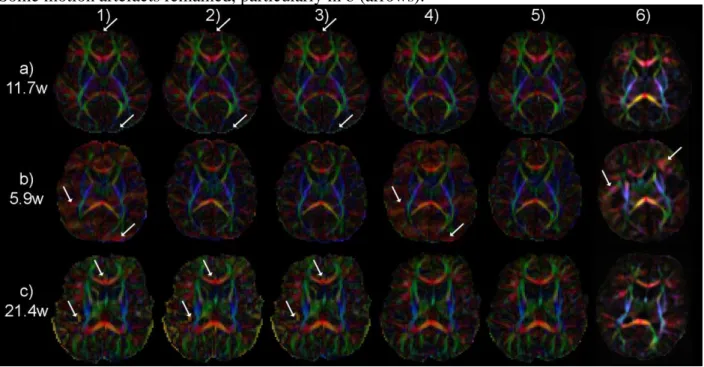
This strategy further improved the quality of resulting DTI maps, as outlined by RGB maps (Figure 5). When outlier slices were either not rejected or resampled (strategies #1 and #4), remaining artifacts were seen with a color-code corresponding to corrupted orientations (see arrows in Figure 5b). The red color (right/left orientation) corresponds to the read echo-train axis that often shows artifacts because it is highly solicited when the DW orientation is along the x-gradient axis. When 3D motion registration was not performed (strategies #1, #2 and #3), the bundles’ delineation was blurred and questionable (see arrows in Figure 5c), particularly in the sub-cortical white matter and the corpus callosum. In quiet infants, all RGB maps were relatively similar, except that the correction of eddy current distortions (strategies #4 and #5) enabled to reduce artifacts over the whole brain and obvious discrepancies at the frontal and occipital borders (see arrows in Figure 5a). Finally, the 2-step strategy provided the maps with the highest quality (Figure 5.5), appearing more reliable and less artefacted than maps obtained after correction with RESTORE (Figure 5.6).
d. Impact of the correction strategies: focus on the developing cortico-spinal tract In all infants, the cortico-spinal tract was finely reconstructed by tractography, similarly with all five correction strategies. All strategies also globally provided equivalent quantification
of mean and maximal parameters over the infant group, on average in the tract section, but standard deviations were the smallest with the 2-step correction strategy because of higher minimal values (Figure 6). Furthermore, the age-related increase in FA was more accurate when motion registration was performed (strategies #4 and #5: R=0.62; strategies #1/2/3: R=0.53/0.48/0.48). The detected increase in anisotropy (+0.004/week of age), and the decreases in mean diffusivity (-4.10-6mm2.s-1/week of age) and transverse diffusivity (-6.10-6 mm2.s-1/week of age) were in good agreement with previous studies [33]. Altogether this suggests that the 2-step strategy (strategy #5) was the most reliable approach to reconstruct the immature cortico-spinal tract and to quantify DTI parameters on average over the tract.
IV.
Discussion
DTI and HARDI techniques are sensitive to motion in two ways. First, because they are based on 2D acquisition, motion artifacts may be observed on isolated slices. In addition, misregistration can occur between DTI volumes because of the successive acquisition of several diffusion orientations, and because of eddy current distortions in EPI images. It seems intuitively important to correct images corrupted by such motion-related artifacts before estimating the diffusion models. Actually, it has been shown that the contributions of motion and noise are of the same order of magnitude at 3T, and that both are influenced by the choice of sampling scheme [18]. Motion is generally due to the subject, some of which being more susceptible to move than others, like infants, children and patients. But artifacts can also result from technical problems: in many MRI systems, instabilities of the gradients can lead to spikes [5], and the table may vibrate due to frequency mechanical resonances, which are stimulated by the low-frequency gradient switching associated with the diffusion-weighting [4]. This leads to corrupted data along specific gradient orientations.
We proposed in this study a post-processing approach relying on two successive and uncorrelated steps, which were first validated by introducing selected motion artifacts or discrepancies on different datasets, and comparing the corrected datasets with reference ones. It was further tested on DW data obtained in non-sedated infants, who frequently move during MRI acquisition: it successfully corrected sets corrupted by motion, while it had lower influence on uncorrupted data.
For intra-slice motion, we implemented an original method to detect and resample corrupted slices. For the outlier detection, a distance measure was defined to compare any DW slice and the corresponding b=0 slice. A natural distance could be a correlation coefficient, but no linear relationship exists between the b=0 and the DW signals which are variable across diffusion orientations [35]. Since mutual information (MI) does not rely on any relationship on the grey level intensity [29], it was a more reliable criterion in order to detect putative outliers for each slice independently. Furthermore, b=0 image was selected as a reference to compute MI coefficients. If it is corrupted, this step would fail: using a DW image (for a specific orientation) would bias the detection for closed orientations, and the product of all DW volumes may be corrupted if a single DW image is artefacted. Nevertheless, this may not be a limiting issue: in the context of single-shell diffusion imaging, b=0 image is required anyway to compute the diffusion model, and in multi-shell imaging it is unlikely that all b=0 images would be corrupted.
With this setting-up, the detection was fully automated and reproducible, and the factor f was the only parameter to be tuned once for a specific protocol. The detection was performed on a slice-by-slice basis. Given the acquisition time of a slice (200ms), intra-slice motion generally corrupts the whole slice: artifacts may not be visible in some regions of the brain, nevertheless it does not imply that the signal sampling is reliable in such regions. Besides, vibration-related
artifacts corrupt clusters of voxels within a slice, but it remains difficult to limit the borders of the regions with impaired signal. Consequently methods which correct the artifacts locally (either on a voxel-by-voxel basis [9, 23] or with a moving average window) may fail to correct the wholeness of such artifacts, and rejecting the whole slice may be more reliable. In this study, only a qualitative comparison between our method and RESTORE was performed, but it appeared that using the diffusion tensor model was quite unsuccessful to detect outliers in both infants and an adult dataset locally corrupted for a specific orientation of the diffusion gradients. Combining the two approaches (MI criteria on the whole slice and local constraint on signal intensity) would be a perspective to improve the outlier detection.
Resampling of the detected outliers can be performed from the non-outlier DW images, either in the image space, or in the Q-space. The former strategy is not adequate because the tissue local microstructure can change significantly between neighbouring slices: interpolating the signal can introduce incoherence, partial voluming effects, and consequently lead to the mixture of heterogeneous populations of fibers. Resampling the corrupted data in the Q-space is more robust. In a recent study Sharman and collaborators [6] also considered this correction strategy after manual detection of the outliers. Two smoothing steps were used: a first spatial smoothing in the image space, using a Gaussian filter, which can only be applied to low b-values acquisitions and a second Q-space smoothing applied to the five closest neighbours using a weighted mean, which restricted the smoothed estimates to a very small quantity of DW data and imposed that they remain of good quality. Following smoothing, Q-space interpolation was performed directly on the spherical shell in the native DW signal space [6]. In our approach, the resampling of outlier slices relied on the decomposition of the DW signal on the modified spherical harmonics basis [36], which is a natural basis on the sphere. Contrarily to the geodesic resampling approach [6], it made use of all non-corrupted data, rather than on a restricted neighborhood. Thus, it required a smaller number of valid data to compute a robust diffusion model estimation, and increased robustness to local corruption on the spherical shell, for instance when DW data contained artifacts around a specific orientation because of gradient system instabilities. Since using a non-parametric model may lead to overfitting of the signal, the spherical harmonics decomposition was limited to the 6th order. In addition, a Laplace-Beltrami regularization term was used to better deal with noise removal and avoid any kind of overfitting with spurious spikes that may be present in the signal acquired on a shell of the Q-space. The resampling was validated for 1 to 5 outlier orientations over 30, leading to small errors in diffusion signal (~5%, Figure 4a) in comparison with acquired images. But it may fail in case of severe motion when most orientations are corrupted, then prospective strategies that adapt the acquisition according to the subject’s motion should be preferred [13].
This correction approach is well indicated for any DW acquisition involving spherical samplings. It can be applied not only to the tensor model, but to most HARDI and multiple shell models since the spherical harmonics decomposition can be generalized to acquisitions with multiple q samplings [36, 37]. For such protocols, our method would be particularly useful because the long acquisition times lead to more probable motion. Besides, the regularization relying on the Laplace-Beltrami operator makes the decomposition implicitly robust to noise, and the novel implementation using a modified LMMSE approach [38] also makes it robust to Rician and non-central Chi noise, which is observed in high b-values acquisitions.
In comparison with the strategy based on visual rejection of whole corrupted volumes, our method presents several advantages. It is fully automated and quick, independent from the experimenter, and is performed slice-by-slice rather than volume-by-volume, which is a particularly suitable when a single slice is corrupted. By introducing outliers on purpose in a set
initially not corrupted by motion, we observed that filling in the missing data was equivalent to rejecting these data in terms of FA estimation, but it performed better when considering the estimation of the main eigenvector direction, particularly for outliers along a specific orientation (vibration). Furthermore, over the whole infant group, the final numbers of corrected volumes were smaller, and the resulting DTI maps were equivalent for both strategies. The main advantage of filling in the missing data was to make the number of DW measurements constant from voxel-to-voxel before the computation of the DTI model. Nevertheless it remained that the number of recovered orientations differed across slices. Besides, as the accuracy of the SH decomposition estimation increases with the spatial distribution of the diffusion orientations, it is important to combine our correction method with DW acquisition strategies that optimize the spatial orientation distribution according to the acquisition time and the motion hypotheses [3, 17].
Our 2-step correction strategy also included a 3D realignment of orientation volumes, misregistered by inter-volume motion and eddy current distortions. The implemented registration was based on mutual information with the mean product of DW images, which appeared to be more robust in comparison with the conventional registration based on b=0 image, and gave reliable results for simulated translations and rotations along the three axis and on real data.
The combination of both the resampling of outlier slices and the registration between orientation volumes was critical [9]. However one may wonder which step should be performed first. On the one hand, if an orientation volume still presents irregularities in the diffusion signal, it will be difficult to realign it in 3D. On the other hand, the resampling of corrupted slices may be wrong if the volume is spatially shifted in comparison with the reference. We performed the outlier resampling first, because this step is made slice-by-slice, and would thus be wrong anyhow should the slices be tilted previously by the 3D registration. Moreover, the initial 3D misregistration that we observed between volumes in all infants was verified to be enough small to guarantee the reliability of the outlier slice resampling.
V.
Conclusion
The 2-step correction strategy was validated on datasets with various motion- and vibration-related artifacts, and it was successfully applied to DTI data of the infant brain. Since no hypothesis on the diffusion model is made, it can be used to correct any dataset acquired over a single shell in the Q-space (eg DTI and HARDI local models) and could be easily extended to multiple-shell acquisitions. So it is worth applying this correction in all DW data with potential sources of artifacts. As an example, it here enabled to reliably study the developing cortico-spinal tract, in agreement with previous studies of unmoved datasets [33].
VI.
Acknowledgements
This work was supported by the Fyssen Foundation (for JD), the Fondation de France (for JD), the Ecole des Neurosciences de Paris (for JD and CP), the Association France Parkinson and the DHOS Inserm-APHP (for CP), the McDonnell Foundation and the Fondation Motrice (for GDL), and the French National Agency for Research (ANR NIBB for GDL, LHP, JFM; ANR Maladies Neurodégénératives et Psychiatriques for CP).
VII.
References
1. Le Bihan, D., et al., MR imaging of intravoxel incoherent motions: application to
diffusion and perfusion in neurologic disorders. Radiology, 1986. 161(2): p. 401-7.
2. Jones, D.K., M.A. Horsfield, and A. Simmons, Optimal strategies for measuring diffusion
in anisotropic systems by magnetic resonance imaging. Magn Reson Med, 1999. 42(3): p.
515-25.
3. Dubois, J., et al., Optimized diffusion gradient orientation schemes for corrupted clinical
DTI data sets. MAGMA, 2006. 19(3): p. 134-43.
4. Gallichan, D., et al., Addressing a systematic vibration artifact in diffusion-weighted MRI. Hum Brain Mapp, 2010. 31(2): p. 193-202.
5. Chavez, S., P. Storey, and S.J. Graham, Robust correction of spike noise: application to
diffusion tensor imaging. Magn Reson Med, 2009. 62(2): p. 510-9.
6. Sharman, M.A., et al., Impact of outliers on diffusion tensor and Q-ball imaging: clinical
implications and correction strategies. J Magn Reson Imaging, 2011. 33(6): p. 1491-502.
7. Dubois, J., et al., The early development of brain white matter: a review of imaging
studies in fetuses, newborns and infants. Neuroscience, in press. DOI 10.1016/j.neuroscience.2013.12.044.
8. Huppi, P.S. and J. Dubois, Diffusion tensor imaging of brain development. Semin Fetal Neonatal Med, 2006. 11(6): p. 489-97.
9. Morris, D., et al., Preterm neonatal diffusion processing using detection and replacement
of outliers prior to resampling. Magn Reson Med, 2011. 66(1): p. 92-101.
10. Holdsworth, S.J., et al., Diffusion tensor imaging (DTI) with retrospective motion
correction for large-scale pediatric imaging. J Magn Reson Imaging, 2012.
11. Kim, D.H., et al., Diffusion-weighted imaging of the fetal brain in vivo. Magn Reson Med, 2008. 59(1): p. 216-20.
12. Jiang, S., et al., Diffusion tensor imaging (DTI) of the brain in moving subjects:
application to in-utero fetal and ex-utero studies. Magn Reson Med, 2009. 62(3): p.
645-55.
13. Herbst, M., et al., Prospective motion correction with continuous gradient updates in
diffusion weighted imaging. Magn Reson Med, 2012. 67(2): p. 326-38.
14. Shi, X., et al., Improvement of accuracy of diffusion MRI using real-time self-gated data
acquisition. NMR Biomed, 2009. 22(5): p. 545-50.
15. Poupon, C., et al., Real-time MR diffusion tensor and Q-ball imaging using Kalman
filtering. Med Image Anal, 2008. 12(5): p. 527-34.
16. Frank, L.R., et al., High efficiency, low distortion 3D diffusion tensor imaging with
variable density spiral fast spin echoes (3D DW VDS RARE). Neuroimage, 2010. 49(2): p.
1510-23.
17. Cook, P.A., et al., Optimal acquisition orders of diffusion-weighted MRI measurements. J Magn Reson Imaging, 2007. 25(5): p. 1051-8.
18. Tijssen, R.H., J.F. Jansen, and W.H. Backes, Assessing and minimizing the effects of noise
and motion in clinical DTI at 3 T. Hum Brain Mapp, 2009. 30(8): p. 2641-55.
19. Sakaie, K.E. and M.J. Lowe, Quantitative assessment of motion correction for high
angular resolution diffusion imaging. Magn Reson Imaging, 2010. 28(2): p. 290-6.
20. Rohde, G.K., et al., Comprehensive approach for correction of motion and distortion in
21. Leemans, A. and D.K. Jones, The B-matrix must be rotated when correcting for subject
motion in DTI data. Magn Reson Med, 2009. 61(6): p. 1336-49.
22. Aksoy, M., et al., Single-step nonlinear diffusion tensor estimation in the presence of
microscopic and macroscopic motion. Magn Reson Med, 2008. 59(5): p. 1138-50.
23. Chang, L.C., D.K. Jones, and C. Pierpaoli, RESTORE: robust estimation of tensors by
outlier rejection. Magn Reson Med, 2005. 53(5): p. 1088-95.
24. Niethammer, M., et al., Outlier rejection for diffusion weighted imaging. Med Image Comput Comput Assist Interv, 2007. 10(Pt 1): p. 161-8.
25. Cointepas, Y., et al., A freely available Anatomist/BrainVISA package for analysis of
diffusion MR data. Proceedings of the 9th HBM Scientific Meeting, New York, USA. NeuroImage, 2003. 19: p. S810.
26. Duclap, D., et al., Connectomist-2.0: a novel diffusion analysis toolbox for BrainVISA. Proceedings of the 29th ESMRMB meeting, 2012: p. 842.
27. Wells, W.M., 3rd, et al., Multi-modal volume registration by maximization of mutual
information. Med Image Anal, 1996. 1(1): p. 35-51.
28. Maes, F., et al., Multimodality image registration by maximization of mutual information. IEEE Trans Med Imaging, 1997. 16(2): p. 187-98.
29. Mangin, J.F., et al., Distortion correction and robust tensor estimation for MR diffusion
imaging. Med Image Anal, 2002. 6(3): p. 191-8.
30. Frank, L.R., Characterization of anisotropy in high angular resolution diffusion-weighted
MRI. Magn Reson Med, 2002. 47(6): p. 1083-99.
31. Descoteaux, M., et al., Regularized, fast, and robust analytical Q-ball imaging. Magn Reson Med, 2007. 58(3): p. 497-510.
32. Perrin, M., et al., Fiber tracking in q-ball fields using regularized particle trajectories. Inf Process Med Imaging, 2005. 19: p. 52-63.
33. Dubois, J., et al., Asynchrony of the early maturation of white matter bundles in healthy
infants: quantitative landmarks revealed noninvasively by diffusion tensor imaging. Hum
Brain Mapp, 2008. 29(1): p. 14-27.
34. Dubois, J., et al., Assessment of the early organization and maturation of infants' cerebral
white matter fiber bundles: a feasibility study using quantitative diffusion tensor imaging and tractography. Neuroimage, 2006. 30(4): p. 1121-32.
35. Mangin, J.F., Entropy minimization for automatic correction of intensity nonuniformity. In IEEE Work, MMBIA, Hilton Head Island, South Carolina, 2000: p. 162-169.
36. Descoteaux, M., et al., Diffusion propagator imaging: using Laplace's equation and
multiple shell acquisitions to reconstruct the diffusion propagator. Inf Process Med
Imaging, 2009. 21: p. 1-13.
37. Assemlal, H.E., D. Tschumperle, and L. Brun, Efficient and robust computation of PDF
features from diffusion MR signal. Med Image Anal, 2009. 13(5): p. 715-29.
38. Brion, V., et al., Parallel MRI noise correction: an extension of the LMMSE to non
central chi distributions. Med Image Comput Comput Assist Interv, 2011. 14(Pt 2): p.
226-33.
Table 1: Summary of the numbers of corrected volumes for the different
strategies.
For each infant, are specified the age and the number of volumes corrected for the four applied strategies in comparison with no correction. For all parameters, the mean and standard deviations over the 20 infants are detailed, as well as the minimum and maximum values.
# age manual
(weeks) rejection dif >0% dif >1% dif >1% dif >5% dif >1% dif >5% 1 5,9 8 2,3 1,5 26,6 15,0 26,6 15,2 2 7,4 0 0,9 0,3 6,2 0,0 6,5 0,1 3 9,7 0 0,9 0,1 15,4 0,0 15,6 0,0 4 9,9 3 1,2 0,3 22,5 6,8 22,5 6,9 5 11,1 3 2,4 0,6 23,3 4,0 23,3 4,3 6 11,3 5 2,2 1,5 28,3 23,2 28,5 23,7 7 11,6 6 3,2 1,7 21,2 7,7 21,4 8,5 8 11,7 0 0,0 0,0 11,2 0,0 11,2 0,0 9 11,7 1 2,5 0,9 8,5 0,3 8,8 0,3 10 12,7 3 1,0 1,0 23,0 12,3 23,3 13,2 11 13,1 0 0,8 0,2 8,3 0,1 8,4 0,2 12 13,3 0 0,2 0,1 6,9 0,0 7,0 0,0 13 13,7 0 0,6 0,3 11,9 0,1 12,0 0,1 14 15,0 2 0,7 0,6 14,9 1,2 15,1 1,6 15 15,6 3 1,9 0,8 17,9 4,0 18,3 4,3 16 16,3 0 0,0 0,0 10,9 0,1 10,9 0,1 17 17,6 0 1,0 0,7 23,6 3,7 23,6 3,7 18 18,0 0 2,2 0,1 8,1 0,0 8,1 0,0 19 21,4 6 1,9 1,5 21,1 5,7 21,4 6,1 20 22,4 0 0,6 0,2 17,6 0,0 17,5 0,1 mean 13,5 2,0 1,3 0,6 16,4 4,2 16,5 4,4 std-dev 4,2 2,5 0,9 0,6 7,1 6,2 7,1 6,4 min 6 0 0,0 0,0 6,2 0,0 6,5 0,0 max 22 8 3,2 1,7 28,3 23,2 28,5 23,7 outlier correction 3D registration 2-step correction Mean count of corrected volumes
Figure 1: Schematic summary of the 2-step correction strategy
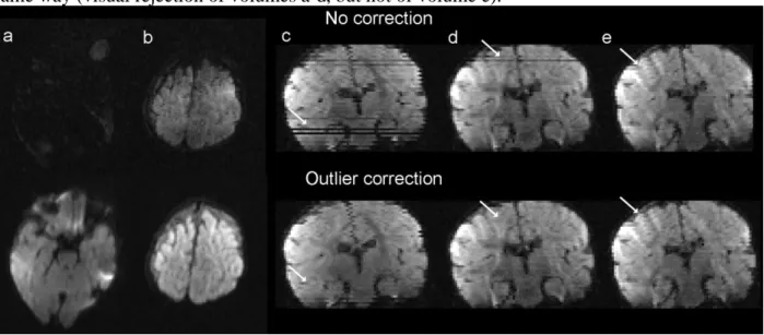
Figure 2: Automated resampling of corrupted slices
DW images of a 21.4w-old infant are presented for different slices and different orientations of the diffusion gradients without any correction (first row) and after resampling for the detected outlier slices with f=3 (second row). Slices are presented in axial (a, b) or coronal views (c-e: arrows in c and d respectively correspond to slices in a and b). Corrupted slices resulting from fast motion during the volume acquisition (a-d) were finely resampled whereas minor irregularities in the diffusion signal (arrow in e) were not corrected. Strategy #2 performed in the same way (visual rejection of volumes a-d, but not of volume e).
Figure 3: Variations of MI coefficients across the diffusion orientations
2.1. Examples of MI distributions are presented for different slices of two infants (quiet infant in Figure 3.1.a, moving infant in Figure 3.1.b), with the mean (diamond signs) and the intervals Mean ± f x StdDev for f=2 (empty triangle signs) and f=3 (filled triangle signs).
2.2. For three infants, averaged MI coefficients are plotted over the 30 orientations for the strategy without correction (blue dots, strategy #1) and for the strategies with resampling of outlier slices (green diamonds, strategy #3), with 3D registration (yellow triangles, strategy #4), and with the 2-step correction (red dots, strategy #5). The first infant (a: # 8 from Table 1) was quietly asleep whereas the two others (b, c: # 1 and 19 from Table 1) moved a little during acquisition (the orientations rejected with strategy #2 are highlighted with stars). In comparison with the other corrections, the 2-step strategy enabled to drastically homogenize the MI coefficients over the 30 orientations.
Figure 4: Validation of the outliers resampling strategy
Deviations from the reference are presented after resampling or excluding 1 to 5 random or vibration-related outliers introduced in an uncorrupted dataset. For deviations in DW signal (Figure 4.a) and in FA (Figure 4.c), mean normalized deviations are presented (left column in %), as well as the percentages of voxels presenting differences larger than 5% (middle column) and 10% (right column). For angle errors in the tensor main direction (Figure 4.b), three classes of voxels are considered according to FA (left column [0.1-0.3], middle column [0.3-0.5], right column [0.5-1]).