A multimodel ensemble approach to assessment of climate change impacts on the hydrology and water resources of the Colorado River basin

(1)

HAL Id: hal-00298804

https://hal.archives-ouvertes.fr/hal-00298804

Submitted on 13 Dec 2006

HAL is a multi-disciplinary open access

archive for the deposit and dissemination of sci-entific research documents, whether they are pub-lished or not. The documents may come from teaching and research institutions in France or abroad, or from public or private research centers.

L’archive ouverte pluridisciplinaire HAL, est destinée au dépôt et à la diffusion de documents scientifiques de niveau recherche, publiés ou non, émanant des établissements d’enseignement et de recherche français ou étrangers, des laboratoires publics ou privés.

A multimodel ensemble approach to assessment of

climate change impacts on the hydrology and water

resources of the Colorado River basin

N. Christensen, D. P. Lettenmaier

To cite this version:

N. Christensen, D. P. Lettenmaier. A multimodel ensemble approach to assessment of climate change impacts on the hydrology and water resources of the Colorado River basin. Hydrology and Earth System Sciences Discussions, European Geosciences Union, 2006, 3 (6), pp.3727-3770. �hal-00298804�

(2)

HESSD

3, 3727–3770, 2006

Colorado River basin climate change impacts N. Christensen and D. Lettenmaier Title Page Abstract Introduction Conclusions References Tables Figures ◭ ◮ ◭ ◮ Back Close

Full Screen / Esc

Printer-friendly Version Interactive Discussion Hydrol. Earth Syst. Sci. Discuss., 3, 3727–3770, 2006

www.hydrol-earth-syst-sci-discuss.net/3/3727/2006/ © Author(s) 2006. This work is licensed

under a Creative Commons License.

Hydrology and Earth System Sciences Discussions

Papers published in Hydrology and Earth System Sciences Discussions are under open-access review for the journal Hydrology and Earth System Sciences

A multimodel ensemble approach to

assessment of climate change impacts on

the hydrology and water resources of the

Colorado River basin

N. Christensen and D. P. Lettenmaier

Department of Civil and Environmental Engineering Box 352700, University of Washington, Seattle WA 98195, USA

Received: 16 November 2006 – Accepted: 28 November 2006 – Published: 13 December 2006

(3)

HESSD

3, 3727–3770, 2006

Full Screen / Esc

Printer-friendly Version Interactive Discussion

Abstract

Implications of 21st century climate change on the hydrology and water resources of the Colorado River basin were assessed using a multimodel ensemble approach in which downscaled and bias corrected output from 11 General Circulation Models (GCMs) was used to drive macroscale hydrology and water resources models.

Down-5

scaled climate scenarios (ensembles) were used as forcings to the Variable Infiltration Capacity (VIC) macroscale hydrology model, which in turn forced the Colorado River Reservoir Model (CRMM). Ensembles of downscaled precipitation and temperature, and derived streamflows and reservoir system performance were assessed through comparison with current climate simulations for the 1950–1999 historical period. For

10

each of the 11 GCMs, two emissions scenarios (IPCC SRES A2 and B1, corresponding to relatively unconstrained growth in emissions, and elimination of global emissions in-creases by 2100) were represented. Results for the A2 and B1 climate scenarios were divided into period 1 (2010–2039), period 2 (2040–2069), and period 3 (2070–2099). The mean temperature change averaged over the 11 ensembles for the Colorado basin

15

for the A2 emission scenario ranged from 1.2 to 4.4◦_{C for periods 1–3, and for the B1}

scenario from 1.3 to 2.7◦_{C. Precipitation changes were modest, with ensemble mean}

changes ranging from −1 to −2 percent for the A2 scenario, and from +1 to −1 per-cent for the B1 scenario. An analysis of seasonal precipitation patterns showed that most GCMs had modest reductions in summer precipitation and increases in winter

20

precipitation. Derived 1 April snow water equivalent declined for all ensemble mem-bers and time periods, with maximum (ensemble mean) reductions of 38 percent for the A2 scenario in period 3. Runoff changes were mostly the result of a dominance of increased evapotranspiration over the seasonal precipitation shifts, with ensemble mean runoff reductions of −1, −6, and −11 percent for the A2 ensembles, and 0, −7,

25

and −8 percent for the B1 ensembles. These hydrological changes were reflected in reservoir system performance. Average total basin reservoir storage generally de-clined, however there was a large range across the ensembles. Releases from Glen

(4)

HESSD

3, 3727–3770, 2006

Full Screen / Esc

Printer-friendly Version Interactive Discussion Canyon Dam to the Lower Basin (mandated by the Colorado River Compact) were

re-duced for all periods and both emissions scenarios in the ensemble mean. The fraction of years in which shortages occurred increased by approximately 20% by period 3 in for both emissions scenarios, and the average shortage increased to a maximum of 3.7 BCM/yr for the period 3 A2 ensemble average. Hydropower output was reduced in

5

the ensemble mean for all time periods and both emissions scenarios.

1 Introduction

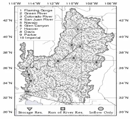
The Colorado River Basin (CRB) includes parts of seven U.S. states and Mexico (Fig. 1). The headwaters lie in the Rocky Mountains of Wyoming and Colorado, from which the river flows some 1400 km to the Gulf of California. It drains a mostly

semi-10

arid region, with an average of only 40 cm/year of precipitation over the 630 000 km2 basin. 70 percent of the Colorado’s flow originates as snowmelt, with the annual hy-drograph dominated by winter accumulation and spring melt. 85 percent of streamflow is generated from 15 percent of the area, while the lower basin (below Lees Ferry, AZ) contributes only 8 percent of the annual streamflow volume. The Colorado River also

15

has considerable temporal variability, with a coefficient of variation for annual stream-flow of 0.33 (by comparison, the coefficient of variation for the Columbia River is less than 0.2). From 1906–2003, annual streamflow had a minimum, maximum, and mean of 6.5, 29.6 and 18.6 billion cubic meters (BCM) at Lees Ferry. A recent 500-year re-construction of Colorado River discharge using tree ring data (Woodhouse et al, 2006)

20

suggests that the long term average annual flow is somewhat lower than for the 1906– 2003 reference period – in the range 17.7–18.1 BCM.

The Colorado River has over 40 major dams and is often described as the most regulated and over allocated river in the world (USDOI, 2000). It has an aggregate reservoir capacity of 74.0 BCM, four times its mean annual flow. 85 percent of basin

25

storage capacity lies in Lakes Powell (formed by Glen Canyon Dam) and Mead (formed by Hoover Dam). The Law of the River which governs management of the river consists

(5)

HESSD

3, 3727–3770, 2006

Full Screen / Esc

Printer-friendly Version Interactive Discussion of 12 major and many minor federal and state laws, treaties, court decisions, and

compacts and divides the basin’s water between the Upper Basin states (Wyoming, Utah, Colorado, and New Mexico), Lower Basin states (Arizona, Nevada, California), and Mexico. The first document of the Law of the River is the Colorado Compact of 1922 which after gauging the river during a period of abnormally high flow apportioned

5

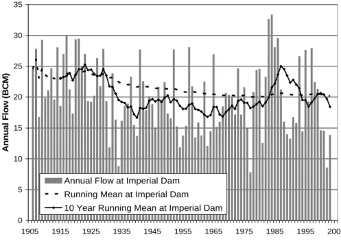
9.3 BCM/yr to both the Upper and Lower Basin. Another element of the Law of the River is the U.S.-Mexico Treaty of 1944 which stipulates that Mexico will receive 1.9 BCM/yr on average at the U.S. – Mexico border. During most of the period since the signing of the compact the 10 year average flow has been below the 20.5 BCM that has been allocated (see Fig. 2) – a situation that is further exacerbated by the estimated

10

1–2 BCM of annual reservoir evaporation. On the other hand, the Compact allocation to the upper basin states has to date not been fully utilized, and for this reason the Law of the River has been able to function notwithstanding the apparent overallocation of the river’s water.

Climate change is a major concern in the CRB due to the sensitivity of discharge

15

to temperature (both through changes in snow accumulation and melt and through in-creased evapotranspiration) which is exacerbated by the semi-arid nature of the basin (Loaiciga, 1996). Global General Circulation Models (GCMs) of the coupled land-ocean-atmosphere system project an increase in global mean surface air temperature between 1.8◦_{C and 5.4}◦_{C between 1990 and 2100 yet disagree upon the tendency and} 20

seasonality of precipitation changes (IPCC, 2001) as well as their spatial distribution regionally. In general, increases in temperature within the Colorado River basin (aside from precipitation increases) will increase the rain to snow ratio, move runoff peaks in the spring, increase evapotranspiration, and decrease streamflow (Christensen et al, 2004). The seasonality of precipitation changes contribute to their effect upon runoff

25

change: a greater percentage of winter precipitation generates runoff than in summer (due to lower evaporative demand).

A previous study of potential climate change in the CRB (Christensen et al., 2004) used the U.S. Department of Energy/National Center for Atmospheric Research

(6)

HESSD

3, 3727–3770, 2006

Full Screen / Esc

Printer-friendly Version Interactive Discussion allel Climate Model (PCM) with a business-as-usual (BAU) global emission scenario

(the most recent (2005) IPCC GCM runs no longer use a BAU scenario, however the A2 scenario used in the results we report here is the closest to BAU of those consid-ered). In Christensen et al. (2004), average temperature changes of 1.0, 1.7, and 2.4◦_C

and precipitation changes of −3, −6, and −3% were predicted for the CRB for periods

5

2010–2039 (period 1), 2040–2069 (period 2), and 2070–2099 (period 3), respectively, relative to 1950–1999 means. These temperature and precipitation changes led to reductions of 1 April snow water equivalent (SWE) of 24, 29, and 30% and runoff re-ductions of 14, 18, and 17% for periods 1–3. Other studies (Gleick, 1987; Lettenmaier et al., 1992; Nash and Gleick, 1991; 1993; Hamlet and Lettenmaier, 1999; McCabe

10

and Hay, 1995; McCabe and Wolock, 1999; Wilby et al., 1999; Wolock and McCabe, 1999) of climate change impacts on hydrology and water resources of western U.S. river basins have used both climate signals from GCMs as well as prescribed tem-perature and precipitation changes. All studies have assumed or predicted increas-ing temperatures, but have disagreed upon both the magnitude and direction of

pre-15

cipitation changes. Aside from Christensen et al. (2004), only one of these studies (Nash and Gleick, 1991; 1993) has been specific to the CRB. Nash and Gleick as-sessed the impacts of a doubling of CO2 concentrations (at the time of their study, so-called transient GCM output was not widely available). In addition, Nash and Gle-ick (1991) evaluated prescribed changes of +2◦

C and +4◦_{C coupled with precipitation} 20

reductions of −10% and −20%. The 2◦_{C increase/10 percent precipitation decrease}

resulted in a 20 percent streamflow reduction while the 4◦_{C increase/20 percent}

pre-cipitation decrease resulted in a 30 percent runoff decrease. A related study by Nash and Gleick (1993) which analyzed scenarios with both increases and decreases in pre-cipitation suggested that slight increases in prepre-cipitation would be offset by increased

25

evapotranspiration, with the net result being reductions in streamflow ranging from 8 to 20 percent. Wolock and McCabe (1999) utilized climate output from GCMs to drive a hydrology model and concluded that a slight increase in precipitation with modest temperature increase would result in decreased streamflow, while for another GCM a

(7)

HESSD

3, 3727–3770, 2006

Full Screen / Esc

Printer-friendly Version Interactive Discussion significant increase in precipitation coupled with a larger temperature increase would

result in increased streamflow. The diversity of scenarios considered by the assortment of climate change studies reflects the considerable uncertainty in the expected amount of warming and in the magnitude and direction of potential precipitation changes.

The managed water resources of the CRB are highly sensitive to runoff reductions

5

due to the almost complete allocation of streamflow to consumptive uses. Increased temperature alone, unless offset by substantial increases in precipitation, will stress the water resources of the CRB, while any precipitation decrease will exacerbate these stresses. Nash and Gleick (1993) found system storage was highly sensitive to changes in runoff, suggesting that the system is currently in a rather fragile balance.

10

Christensen et al. (2004) found that runoff reductions of 14–18 percent resulted in sys-tem storage reductions of 30–40 percent and target releases from Glen Canyon Dam being met 17–32 percent less often than in the reference (1950–99) historic period. Nash and Gleick (1993) found that violations of the Compact would occur if average runoff dropped by only 5 percent. On the one hand, the large storage to runoff ratio

15

of the basin mitigates the effects of seasonal shifts in runoff timing associated with a warmer climate; however, the large storage capacity will have little effect on long term reliability of water deliveries if average flows decline.

The present study utilizes 11 GCMs under IPCC (2006) emission scenarios SRES A2 and B1, where A2 corresponds to relatively unconstrained growth in global

emis-20

sions, and B2 corresponds to elimination of global emissions increases by 2100. Each GCM’s historical simulation was used to bias correct and downscale the temperature and precipitation signals from the A2 and B1 scenarios using methods outlined in Wood et al., (2002) and Wood et al., (2004). The bias corrected and downscaled temperature and precipitation signals were then used to drive the Variable Infiltration Capacity (VIC)

25

macroscale hydrology model (Liang et al., 1994; Nijssen et al, 1997) at a daily time step. Monthly aggregates of VIC-simulated streamflow model at selected reservoir in-flow points (Fig. 1) were used to force the CRRM. CRRM, described in more detail in Christensen et al. (2004) is a simplified version of the Colorado River Simulation

(8)

HESSD

3, 3727–3770, 2006

Full Screen / Esc

Printer-friendly Version Interactive Discussion tem (USDOI, 1985). It predicts storage in the main CRB reservoirs, and deliveries of

water to major water users, as well as hydropower generation. We summarize results of both the VIC and CRRM simulations for period 1 (2010–2039), period 2 (2040–2069, and period 3 (2070–2099), and compare them with a “historical” simulation driven by 1950–1999 observations.

5

2 Approach

2.1 General circulation models and emission scenarios

The 11 GCMs which produced the climate scenarios used in this study are summarized in Table 1, which includes references to the details of each model. Although many other GCM runs have been prepared for IPCC, these 11 model runs are the most

10

consistent in terms of the future simulation period (all were run for at least the period 2000–2100), and the emissions scenarios used. These GCMs represent the major global modeling centers and provide the basis for the most thorough climate study of the Colorado River basin to date. In that respect, we note that our approach here is a generalization of Christensen et al. (2004), who ran one model and emissions

15

scenario for the CRB using essentially the same methods as were used in this study, and Maurer et al. (2006), who ran 10 of the same 11 models we use, and the same emissions scenarios for California.

For its Fourth Assessment Report (AR4), the IPCC created six plausible global greenhouse gas emissions scenarios; A1F, A1B, A1T, A2, B1, and B2. With respect to

20

global emissions of greenhouse gases (and hence, in general, global average temper-ature increases) from warmest to coolest are scenarios A1FI, A2, A1B, B2, A1T, and B1. The A2 and B1 scenarios were chosen for this study because they are the most widely simulated over all models (not all modeling groups have archived runs for all emissions scenarios), and because they represent a plausible range of conditions over

25

(9)

HESSD

3, 3727–3770, 2006

Full Screen / Esc

Printer-friendly Version Interactive Discussion In the A2 scenario, global average CO₂concentrations reach 850 ppm by 2100, while

in the B1 scenario CO2 concentrations initially increase at nearly the same rate as in

the A2 scenario, but then level off around mid-century and end at 550 ppm by 2100. Christensen et al. (2004) used the Parallel Climate Model (PCM) under an emissions scenario (not included in the model runs summarized in Table 1) that lies between A2

5

and B1.

Details of the bias correction and downscaling approach used to translate GCM out-put into VIC inout-put are reported in Wood et al (2002; 2004) and Maurer et al. (2006). In brief, the method downscales monthly simulated and observed temperature and pre-cipitation probabilities at the GCM spatial scale (regridded to a common 2 degrees

10

latitude by longitude spatial resolution) to the 1/8 degree resolution at which the VIC hydrology model was applied through use of a probability mapping procedure that is “trained” to monthly empirical probability distributions of the climate model output for current climate conditions to equivalent space-time aggregates of the gridded (one-eighth degree spatial resolution) observation set of Maurer et al. (2002). The climate

15

model signal was then temporally and spatially disaggregated through use of a resam-pling approach to create a daily forcing time series for the hydrology model at the same one-eighth degree spatial resolution. This method facilitates investigation of the impli-cations of the true transient nature of climate warming as opposed to the more common methods employed where decadal temperature and precipitation shifts are averaged to

20

give a step-wise evolution of climate (e.g. Hamlet and Lettenmaier, 1999). 2.2 VIC model application to the CRB

Liang et al. (1994) and Nijssen et al. (1997) provide details of the VIC model and its application to continental river basins, while Christensen et al. (2004) provide details of its application to the Colorado River basin, hence our description here is highly

25

condensed. VIC is a grid cell based macroscale hydrology model that typically runs at spatial resolutions ranging from one-eighth to two degrees latitude by longitude. The VIC model is forced by gridded temperature, precipitation, and wind time series,

(10)

HESSD

3, 3727–3770, 2006

Full Screen / Esc

Printer-friendly Version Interactive Discussion as well as other surface radiative and meteorological variables that are derived from

daily mean temperature and temperature minima/maxima following methods outlined by Maurer et al. (2002). The VIC model can be run either at a sub-daily time step which facilitates a full energy balance, or (as was used in this study) at daily time step in water balance mode. The model simulates soil moisture dynamics, snow accumulation and

5

melt, evapotranspiration, and generates surface runoff and baseflow which are subse-quently routed through a grid based river network to simulate streamflow at selected points within the basin.

As in Christensen et al. (2004), VIC grid cell runoff was routed to locations repre-senting the inflow to seven major reservoirs and three inflow-only locations used in the

10

reservoir simulation model (Fig. 1). VIC was calibrated by adjusting parameters that govern infiltration and base flow recession to match simulated historic streamflow with naturalized observed obtained from the U.S. Bureau of Reclamation (2000) at selected points for the same period of record. The overlapping period of record between simu-lated and observed naturalized streamflow is 1950–1999, during which VIC cumulative

15

simulated streamflow was 768 BCM and observed naturalized was 776 BCM. This rep-resents a bias within VIC to slightly underpredict streamflow (by about one percent). The relative biases at Green River, UT and the Colorado River near Cisco, UT, were slightly larger (3 and −9%, respectively). The additional step of first bias correcting these streamflows before driving CRRM with them has been added since the

Chris-20

tensen et al. (2004) study. Snover et al. (2003) provide details, but this step essentially maps between simulated and observed probability distributions at each CRRM inflow point in each calendar month during the overlapping 1950–1999 period. This same re-lationship is then applied to the future GCM runs, therefore eliminating any systematic spatial bias.

25

2.3 CRRM implementation

CRRM is a simplified version of the U.S. Bureau of Reclamation’s (USBR) Colorado River Simulation System (CRSS) (Schuster, 1987; USDOI, 1985) developed by

(11)

Chris-HESSD

3, 3727–3770, 2006

Full Screen / Esc

Printer-friendly Version Interactive Discussion tensen et al. (2004) for assessment of the affects of altered streamflow regimes on

performance of the Colorado River reservoir system. CRRM is driven by naturalized streamflow (VIC output) at the inflow at points shown in Fig. 1. It represents all major physical water management structures in the CRB. Pre-specified operating policies are used to simulate reservoir levels and releases, hydropower production, and diversions

5

on a monthly time step.

Because of the large fraction of total CRB reservoir storage in Lakes Powell and Mead, not all of the physical or operational complexities of the river system need to be represented in CRRM to enable the assessment of climate change implications of reservoir system performance. CRRM therefore represents the CRB reservoir

sys-10

tem with four storage and three run-of-the-river reservoirs. The storage reservoirs are Flaming Gorge, Navajo, Lake Powell, and Lake Mead, of which only Lakes Powell and Navajo are essentially equivalent to the true reservoirs. Flaming Gorge includes the storage capacity of Fontenelle and Lake Mead includes the storage capacity of the downstream reservoirs that are treated as run-of-the-river in CRRM. Hydropower is

15

simulated at all reservoirs except Navajo and Imperial.

As noted above. the operating policies of the CRB reservoir system are dictated by the Law of the River. In CRRM, like CRSS, these laws have been simplified so that the main regulations affecting operations are a mandatory release of 10.2 BCM per year from Glen Canyon Dam (for the Lower Basin’s 9.2 BCM/yr entitlement and

one-20

half of Mexico’s 1.9 BCM/yr) and an annual release from the Lower Basin to Mexico of 1.9 BCM. CRRM, again like CRSS, requires the release from Lake Powell regardless of the reservoir level relative to its minimum power pool; only when it is not physically possible to release water (dead storage) are releases to the Lower Basin curtailed. CRRM shortage delivery operations were updated in CRRM relative to the version of

25

the model used in Christensen et al. (2004) to reflect the “basin states alternative” (BSA) which is likely to be adopted as the basis for water deliveries in the future. The BSA has three different shortage levels (494, 617, and 740 MCM/yr that are imposed at Lake Mead elevations of 327.66, 320.05, and 312.42 m, respectively. The BSA also

(12)

HESSD

3, 3727–3770, 2006

Full Screen / Esc

Printer-friendly Version Interactive Discussion stipulates a hard protect of the Southern Nevada’s Water Authority (SNWA) intake at

an elevation of 304.80 m. At this elevation deliveries to the lower basin will be reduced, to zero if need be, to ensure no further reduction of elevation. The first three reductions are weighted 79% to CAP, 17% to Mexico, and 4% to SNWA. The BSA does not stip-ulate how shortages are allocated after the 740 MCM/yr level; however CRRM follows

5

the Law of the River and recognizes CAP allocation to be junior to the MWD, which in turn is junior to the Imperial Irrigation District (IID). CRRM, like CRSS, does not im-pose shortages on the Upper Basin but rather passes them onto the Lower Basin even though this could be considered a violation of the Law of the River (Hundley, 1975).

Water demands in this study were based on the USBR’s Multi-Species Conservation

10

Program (MSCP) (USDOI, 2000) baseline demands for year 2000. Upper Basin de-mands were fixed at 5.2 BCM/yr and Lower Basin at their full entitlement of 9.2 BCM/yr. Although demands will likely increase as population increases in the basin, holding demands steady allows us to isolate the effects climate change from the confounding effects of transient demand increase. CRRM represents withdrawals from the river at

15

11 diversion points, each of which has a unique monthly return ratio (fraction of water diverted that is returned to the river). If there is insufficient water within a river reach or reservoir to meet a demand, the two upstream reservoirs are allowed to make re-leases to fulfill the demand. Present perfected water rights are not explicitly modeled in CRRM, instead priority is given to upstream users except in the case of Lower Basin

20

shortages.

Christensen et al. (2004) show validation plots of CRRM during the period 1970– 1990, in which it had a 1 percent monthly storage error and a 0 percent accumulated error. During this period it had a 12 percent accumulated hydropower error, but the error was largely due to the high reservoir levels in the mid-80s coupled with CRRM’s

25

lack of inflow forecasting. Given results reported in the following section, it appears unlikely that these high reservoir levels will be reached in the future, so CRRM arguably represents hydropower production adequately for the purpose of this study.

(13)

HESSD

3, 3727–3770, 2006

Full Screen / Esc

3 Results

In this section we analyze downscaled and bias corrected GCM climate scenarios (us-ing the method of Wood et al, 2004) which we compare to 1950–1999 gridded historical observations of daily temperature and precipitation from Maurer et al. (2002). Hydro-climatic variables (runoff, SWE, evaporation) simulated by VIC for the GCM scenarios

5

are compared to VIC simulations driven by the 1950–1999 climate observations. Base-line statistics for the 1950–1999 period are termed “historical”, while GCM results are divided into period 1 (2010–2039), period 2 (2040–2069), and period 3 (2070–2099). 3.1 Downscaled climate change scenarios

Figure 3 shows the transient basin average temperature for each of the 11 GCMs

10

throughout the 21st century under both the A2 and B1 emission scenarios. Although there is considerable spread within each scenario, it is apparent that by the second half of the century there is significantly more warming associated with the A2 than the B1 scenario. By period 2, all the climate models with the exception of PCM simulate warmer temperatures for the A2 scenario, and by period 3 all GCMs simulate warmer

15

A2 temperatures (average warming of 2.7◦_{C in B1 vs. warming of 4.4}◦_{C in the A2}

scenario). Table 2 summarizes ensemble average changes while Tables A.1 and A.2 report results for individual ensemble members.

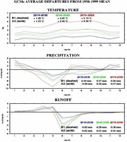
Figure 4 shows the shift in annual distribution of temperature and precipitation, and resulting runoff for periods 1–3 relative to the 1950–1999 historic simulation. Results

20

are presented for the ensemble average and 1st and 3rd quartiles. As expected (be-cause A2 and B1 emission scenarios are similar for the first part of the century) there is little difference in warming between the two scenarios during period 1. The ensemble average B1 period 1 warming is 1.28◦_{C (1st and 3rd quartiles 1.02 and 1.67}◦_{C) while}

A2 is 1.23◦_{C (0.95, 1.49}◦_{C). By period 2 the B1 scenario has a mean shift of 2.05}◦_C 25

(1.64, 2.48◦_{C). In the same period, the mean A2 shift is 2.56}◦_{C (1.94, 2.83}◦_{C). By}

pe-riod 3, scenario A2 is 1.7 ◦_{C warmer than B1. B1 has a mean shift of 2.74}◦_{C (1.89,}

(14)

HESSD

3, 3727–3770, 2006

Full Screen / Esc

Printer-friendly Version Interactive Discussion 3.23◦_{C) while A2 is 4.35}◦_{C (3.32, 5.38}◦_{C). The ensemble averages for all scenarios}

and time periods have more warming from mid-summer to early fall, which may be at-tributable to fact that there is less moisture during these months than in the historical simulation, and therefore more energy going to sensible than to latent heating.

Averaged over all GCMs (“ensemble average”), changes in average annual

precip-5

itation are −1 (−6, +3), −2 (−7, +7), and −2 (−8, +5) percent for the A2 scenario, and +1 (−3, +6), −1 (−6, +4), and −1 (−8, +2) percent for the B1 emission sce-nario for periods 1–3, respectively (Fig. 5). Although annual precipitation decreases the ensemble average winter precipitation volume increases (Fig. 4b). The increase in winter precipitation (quantified as Oct–March ensemble total precipitation volume

rel-10

ative to Oct–March base run total precipitation volume) is 5, 1, and 2 percent for the B1 scenario, and 6, 5, and 4 percent for the A2 scenario for periods 1–3, respectfully. Upstream of Lees Ferry (where a larger percentage of precipitation results in runoff), the B1 scenario has a 7 percent precipitation increase in period 1 and 6 and 8 percent increases in periods 2 and 3. In the A2 scenario, the increase in precipitation upstream

15

of Lees Ferry is 8, 10, and 14 percent in periods 1–3, respectively. In Sect. 3.4 we per-form a separate sensitivity analysis of the implications of these changes, but in short, a shift towards winter precipitation results in more runoff for a given precipitation amount. These increases in winter precipitation amounts are opposite to the projections by the earlier version of PCM utilized in Christensen et al. (2004). The ensemble averages

20

in that study had winter precipitation decreases of 4, 6, and 4 percent for periods 1–3, respectfully, which drove much larger reductions in (annual) streamflow than projected in this study (see below).

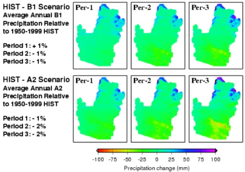
Figure 5 shows the spatial distribution of predicted changes in annual precipitation. Increases are predominantly in the high elevation areas of the Rockies in Colorado,

25

Wyoming and Utah while decreases are greatest in the desert portions of the south-east basin in Arizona and New Mexico. It should be noted that the fine spatial resolution of the predicted precipitation changes in Fig. 5 is in fact driven by the coarse spatial resolution of the GCM output. The regions in Fig. 5 that show the greatest

(15)

precipita-HESSD

3, 3727–3770, 2006

Full Screen / Esc

Printer-friendly Version Interactive Discussion tion increases are in general the areas that have high precipitation in the same months

for which the GCMs predict increases. The mountainous headwaters regions, for ex-ample, receive a preponderance of their precipitation in the winter, and because the GCMs on average have winter precipitation increases, the Rockies have the greatest annual average precipitation increases. The converse holds for summer; decreases

5

in basin wide summer precipitation cause the greatest annual (volume) reductions to occur in the southeast since this region receives most of its rainfall during the sum-mer months. It should also be noted that due to the number of GCMs, periods, and emission scenarios, the spatial plots presented are for ensemble averages.

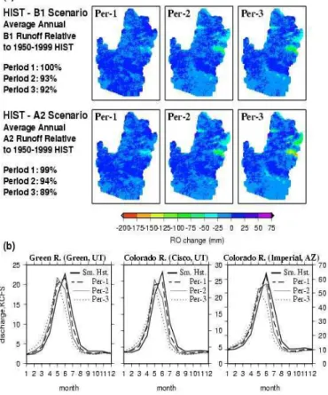
3.2 Runoff changes

10

Figure 6a shows spatial changes in the ensemble average mean annual runoff for peri-ods 1–3 relative to simulated historic, and Fig. 6b shows the mean monthly hydrograph for three streamflow locations in the basin. 1950–1999 basin average annual precipita-tion is 354 mm, of which 310 mm evaporates, leaving 45 mm to runoff. This constitutes a runoff ratio of around 13 percent which is typical of semi-arid watersheds (Nash and

15

Gleick, 1991). Runoff stays essentially unchanged in period 1 for both SRES scenar-ios, decreases by 7 (−15, 0) and 6 (−14, +8) percent in period 2 for the B1 and A2 scenarios, respectively, and by 8 (−18, −1) and 11 (−16, −1) percent in period 3 for the B1 and A2 scenario. Table 2 shows average annual precipitation, evaporation, and runoff in mm/year, and runoff ratio and basin average annual temperature. Although

20

precipitation changes are modest (+1 to −2 percent), changes (mostly decreases) in runoff ratio are larger. The runoff ratio reductions are driven both by temperature (the higher the temperature, the lower the runoff ratio) as well as by shifts in the season-ality of precipitation (see Sect. 3.4). For individual GCM ensemble members in which there are comparable temperature and precipitation changes, the runs that have larger

25

shifts towards winter precipitation have higher runoff ratios. In Christensen et al. (2004) we utilized an earlier version of PCM which projected slightly greater precipitation creases, smaller temperature increases, and from which substantially larger runoff

(16)

HESSD

3, 3727–3770, 2006

Full Screen / Esc

Printer-friendly Version Interactive Discussion creases were inferred. For period 3 annual average temperature increases of 2.4◦_C

and precipitation decreases of 3 percent drove a runoff decrease of 17 percent. As noted above, this large runoff decrease for the modest temperature and precipitation change (relative to the ensemble means in this study) is a result in large part of the earlier PCM’s shift away from winter precipitation. Nonetheless, although a reduction

5

of 5 mm/year of runoff may seem modest, it represents a reduction of 11 percent which has major implications on a system which is already over-allocated.

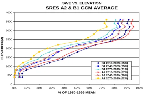
3.3 Snowpack changes

Basin average 1 April snow water equivalent (SWE), the depth of water that the snow-pack would produce if melted, declines by 13 (25, 6), 21 (29, 16), and 38 (48, 19)

10

percent in scenario A2, and by 15 (24, 11), 25 (31, 18), and 29 (33, 19) percent in scenario B1 in periods 1–3, respectively. Winter precipitation is greater for all ensem-ble means relative to the historical period, leading to the conclusion that the reductions in SWE are directly attributable to higher winter temperatures and the resulting de-crease in the ratio of precipitation falling as snow vs. rain. Reductions in SWE present

15

are greatest in the low to mid elevation transitional zone (Fig. 7). The metric “snow present” is a function of both SWE depth and the amount of time the SWE is present. If an equivalent amount of snow falls, but melts twice as fast, it is considered 50% of his-torical. These results are consistent with Nash and Gleick (2003), Wilby et al. (1999), McCabe and Wolock (1999), Brown et al. (2000), and Christensen et al. (2004).

20

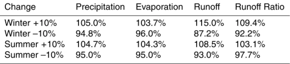
3.4 Sensitivity of runoff to seasonality of precipitation

A separate analysis was performed to better understand the effect that a seasonal shift in precipitation would have on runoff generation. To do this we compared runoff gener-ated by a base run to simulations in which winter (Oct–March) and summer (April–Sep) precipitation was individually increased and decreased by 10 percent (Table 3). The

25

(17)

precipita-HESSD

3, 3727–3770, 2006

Full Screen / Esc

Printer-friendly Version Interactive Discussion tion results in runoff Comparison of Tables 2 and 3 suggests that 38 percent of the

increase in winter precipitation results in runoff, while only 23 percent of the summer precipitation increase contributes to streamflow. The same trend holds for precipita-tion decreases, with comparable decreases in precipitaprecipita-tion leading to almost twice as much runoff decrease in winter than summer. This analysis confirms that the slight

5

shift towards increased winter precipitation in the ensemble means helps offset some of the effects of increased temperatures ratios on evapotranspiration.

3.5 Reservoir system performance

The managed water resources of the Colorado River Basin are extremely sensitive to changes in the mean annual flow of the river due to its almost complete allocation of

10

streamflow to consumptive uses. As noted above, the Colorado River Compact of 1922 was based on abnormally high flow years in which the average streamflow of the river was around 22.2 BCM/yr, of which 20.4 BCM/yr was allocated to consumptive use. The results we report are based on consumptive use of 17.5 BCM/yr (Mexico and the Lower Basin utilizing their full allocation, and the Upper Basin fixed at their actual year 2000

15

consumptive use of 6.4 BCM/yr). Annual reservoir evaporation is a function of storage (i.e. surface area), however it is on average greater than one BCM per year, making total consumptive losses (use+evaporation) over 18.8 BCM/yr.

The 1906–1999 average discharge of the river at its mouth (without regulation) would be 20.4 BCM/yr, with 10-year average flows as low as 16.3 BCM/yr, however the

sys-20

tem has been able to operate reliably in the past due to Upper Basin demand being lower than current levels. Any reduction in streamflow will exacerbate the stress of in-creasing Upper Basin demands and reduce system reliability. In 32 of the 66 ensemble members (2 SRES scenarios, 3 time periods, 11 climate models), average streamflow is below the current consumptive use (domestic depletions plus reservoir evaporation

25

plus Mexico release) of 18.8 BCM/yr. In only eight of the B1 ensembles and six of the A2 ensembles (none in 2070–2099) are there no delivery shortages.

We assess changes in reservoir system performance associated with the future 3742

(18)

HESSD

3, 3727–3770, 2006

Full Screen / Esc

Printer-friendly Version Interactive Discussion climate ensembles through the next century by comparing CRRM output for

simula-tions driven by future VIC streamflow sequences with CRRM simulasimula-tions driven by VIC 1950–1999 historical simulations. We show results in this section for total basin stor-age, water delivery reliability, Law of the River compliance, and hydropower production. It should be noted that the historic reservoir simulation has lower average storage

5

and hydropower generation than ensembles that have essentially the same average streamflow. This is a result of the early part of the 1950–1999 record having low inflow, and therefore starting with low storage (head in the case of hydropower). In these simulations, initial reservoir storage was iterated so that the starting value was the same as the average over the 50-year base period. This contrasts with Christensen et

10

al. (2004) who used initial storage equal to the 1970 historic (actual) level. 3.5.1 Storage

Figure 8 shows average 1 January storage as a function of streamflow for each stream-flow ensemble by period and scenario, as well as the streamstream-flow and storage from Christensen et al. (2004), and storage-streamflow combinations from runs in which the

15

base run streamflows were altered in increments of 10 percent from −50 percent to +50 percent. The black dotted line shows that for a given streamflow sequence an increase or decrease of 10 percent in average streamflow is magnified into an increase or de-crease of about 20 percent in average basin storage, and that a 20 percent change in streamflow results in roughly a 40 percent storage change. Results for each of the

en-20

sembles generated for this study follow this general pattern, although the sensitivities when averaged across ensembles are somewhat different than implied by the dashed line. Again, this is primarily a result of the base run having low average storage relative to its average streamflow (because of the low flows early in the sequence).

Although average streamflow in period 1 for both SRES scenarios is less than the

25

base run, CRRM simulates slight ensemble average reservoir level increases of 4 (−20, 23) and 1 (−13, 15) percent for A2 and B1, respectively (Table 4). In period 2, stream-flow changes of −6 (−14, 8) and −7 (−15, 0) percent drive 1 January storage changes

(19)

HESSD

3, 3727–3770, 2006

Full Screen / Esc

Printer-friendly Version Interactive Discussion of −1 (−40, 22) and −5 (−42, 32) percent for the A2 and B1 scenarios, respectively,

while period 3 changes in streamflow of −11 (−16, −1) and −8 (−18, −1) percent drive storage changes of −13 (−39, +9) and −10 (−46, +20) percent for A2 and B1, respectively (Tables A3 and A4 provide results for individual ensemble members). It should be noted that there are many nonlinearities in the relationship between reservoir

5

performance and inflows (and in fact, the clustering of the points in Fig. 8 around the dashed line is somewhat tighter than one might expect for this reason). For example, in Fig. 8, the B1 period 3 simulation (IPSL) in which 90 percent of base streamflow drives reservoir storage of 120 percent of base is a function of very high initial reservoir lev-els (>56 BCM) and very high early period streamflow and low late period streamflow.

10

Another outlier in Fig. 8 is the B1, period 1 simulation (MRI) in which 110 percent of base streamflow drives a storage reduction. This is a result of MRI having very low streamflow prior to 2010 and a result, total initial reservoir storage of only 17 BCM.

Although these results seem inconsistent with the greater storage reductions pre-dicted by Christensen et al. (2004), they are within the same range of sensitivity.

Chris-15

tensen et al. (2004) predicted streamflow reductions at the high end of those simulated for individual ensemble members for this study, and as can be seen in Fig. 8, storage reductions in these ensemble members match those of the 2004 study.

3.5.2 Delivery compliance

Water deliveries are dependent on the storage in Lake Mead; level one shortages are

20

imposed (see Sect. 2.3 for amounts and to which users) when Lake Mead drops below an elevation of 327.66 m, level two shortages are imposed at an elevation of 320.04 m, and level three at 312.42 m. If need be, deliveries are decreased further to ensure that the elevation of Lake Mead does not drop below the SNWA’s intake at 304.80 m elevation.

25

Figure 9 shows the average shortage per year, the percentage of years with no shortages, and the percentage of years with level three shortages for the 1950–1999 “base” run and for the SRES A2 and B1 ensemble averages for periods 1–3. The

(20)

HESSD

3, 3727–3770, 2006

Full Screen / Esc

Printer-friendly Version Interactive Discussion base run has delivery shortages in 26 percent of years. In reality, there have not

yet been shortages, but they are simulated in the base run here because we force CRRM with 1950–1999 streamflow and year 2000 demands. Shortages are simulated in the base run between the late 50s and mid 70s, while in real operations upper basin demands were lower and there were no shortages. The A2 and B1 scenarios both

5

have shortages in 21 percent of years in period 1, 31 and 35 percent of years in period 2, and 38 and 42 percent in period 3.

Level three shortages beginning at 740 MCM/yr are initially imposed when Lake Mead drops below 312.42 m, but are allowed to increase up to the entirety of the Lower Basin and Mexico’s demand to protect a Lake Mead elevation of 304.80 m. The

prob-10

ability of these shortages, along with the average shortage amount (Fig. 9), are not influenced much by the nuances of the reservoir model (initial storage, streamflow se-quence, etc). They are also likely to have considerable socio-economic effect within the basin. Level three shortages are imposed in the base run in 5 percent of years, and in 11 and 10 percent in period one, 24 and 27 percent in period two, and 27 and

15

26 percent in period three for the SRES A2 and B1 ensemble averages, respectively. The shortfall per year (MCM/yr) is derived by dividing the total shortfall in each period by the number of years in which any shortage delivery is imposed. It is a somewhat redundant metric because it is related to the number of level three shortages, however it is important to differentiate between length modest shortfalls and short intense ones.

20

The average shortage in the base run was 0.73 MCM, and 2.1 and 2.0 MCM/yr in period one for the A2 and B1 scenario, respectively. Average shortfalls in period two were 4.2 and 2.1 MCM/yr, and 3.7 and 2.8 MCM in period three for A2 and B1, respectively. Although there seems to be a lack of correlation between streamflow and average shortage (e.g. SRES A2, period 2 has greater streamflow than B2 period 3, yet higher

25

average shortage), this is entirely an artifact of averaging across ensembles. Tables A3 and A4 summarize individual GCM run results.

(21)

HESSD

3, 3727–3770, 2006

Full Screen / Esc

Printer-friendly Version Interactive Discussion 3.5.3 Hydropower generation

Hydropower generation is a function of head (height of water surface above tailwa-ter elevation) and discharge (volume per unit time) passing through a turbine. Be-cause of the sequencing of the base run streamflow and its bias towards lower storage (i.e. head) for a given inflow, it generates less hydropower than the period one A2 and

5

B1 average (Fig. 10). The average energy generated in the base run is 8480 GW-h/yr, while in period one the A2 scenario average generates 8600 GW-h/yr, and in the B2 scenario average 8530 GW-h/yr. In period two, the A2 average is 7630, and the B1 average is 7560 GW-h/yr, while in period three A2 is 6900 and B1 is 7130 GW-h/yr. The reduction of hydropower production from period 1 to period 3 is 20 percent in

10

the A2 scenario and 16 percent in the B1 scenario, both of which are about twice the corresponding streamflow reduction percentages.

3.5.4 Glen Canyon Dam and Mexico release

The Colorado River Compact mandates a 10 year moving average release of 10.2 BCM/yr from the Upper Basin to the Lower Basin and an annual release of

15

1.9 BCM (1.5 MAF) from the United States to Mexico. Figure 10 and Table 4 report the detailed results, but in general releases from Glen Canyon Dam are 1 percent less (both B1 and A2) in period one than in the historical run and 7 and 8 percent lower in period 2 for B1 and A2, respectively. Period 3 has an 8 percent reduction in Glen Canyon releases in the B1 scenario, and a 12 percent reduction in A2. Although the

20

compact requires the 10.2 BCM/yr release to be made on a 10 year moving average, current basin operations dictate that this release is made annually. The Glen Canyon release drops below 10.2 BCM in 24 percent of years in the base run, and 28, 35, and 35 percent of years for the B1 scenario in periods 1–3, respectfully. The Glen Canyon release drops below 10.2 BCM/yr in 28, 34, and 44 percent of years in the A2 scenario

25

for periods 1–3, respectfully.

Mexico is allocated (in the model) 17 percent of the level one through three shortage 3746

(22)

HESSD

3, 3727–3770, 2006

Full Screen / Esc

Printer-friendly Version Interactive Discussion amount, so the amount of years in which the Lower Basin delivery to Mexico drops

below 1.9 BCM is essentially the same as the percentage of years in which any short-ages are imposed (see Sect. 3.5.2). The average delivery to Mexico in the base run is 1.8 BCM/yr, while the B1 scenario average annual deliveries drop to 1.78, 1.72, 1.65 BCM for periods 1–3 respectfully. In periods 1–3 of the A2 scenario, average

5

annual deliveries are 1.78, 1.63, 1.62 BCM, respectfully.

4 Conclusions

As compared with earlier studies of climate sensitivity of CRB water resources to cli-mate change, we have assessed in detail the implications of eleven downscaled IPCC climate model scenarios and two emissions scenarios, each one of which constitutes

10

an ensemble member. Therefore, we are able to evaluate the range of possible con-sequences as represented by the different models and emissions scenarios, including “consensus” (mean) results, and measures of variability, in particular, the lower and upper quartiles. In this respect, this study is the most comprehensive to date of the implications of climate change on the Colorado River reservoir system.

15

As in essentially all previous studies, average annual temperatures over the CRB increase with time, not only in the ensemble mean, but for all individual climate models and time period. With the exception of the early part of the century when the A2 and B1 emission scenarios are similar and natural variability can dominate the emissions signal, temperatures are greater for the A2 emission scenario than for B1. Average

20

temperature increases for the period 2070–2099 are 2.75◦

C (with a range of +/−1.0◦_C)

for the B1 scenario and 4.35◦

C (+/−1.5◦_{C) for the A2 scenario.}

While all models agree with respect to the direction of temperature changes, there is considerable variability in the magnitude, direction, and seasonality of projected precip-itation changes. Averaged over models, annual precipprecip-itation changes are quite small –

25

a maximum change (decrease) of 2 percent for period 2 and 3 for the A2 emissions sce-nario. The variability across models is, in general, much larger than the annual change.

(23)

HESSD

3, 3727–3770, 2006

Full Screen / Esc

Printer-friendly Version Interactive Discussion More apparent in the ensemble means are shifts in seasonality of precipitation, which,

in the ensemble mean, all show a shift towards more winter and less summer precipi-tation. Because winter precipitation (especially in the upper basin) contributes propor-tionately more to runoff than does summer precipitation, these shifts tend to counteract reductions in annual runoff that otherwise would result from increased temperatures

5

(hence evapotranspiration) This shift toward winter precipitation is prevalent in the en-semble average for all periods and scenarios and is most pronounced for the basin upstream of Lees Ferry. Nonetheless, while this shift reduces the effect of increased temperatures on runoff, it does not reverse them, and in the ensemble mean streamflow decreases for all periods on both emissions scenarios.

10

Runoff changes are driven by combined effects of temperature and precipitation changes and their seasonality. In the ensemble means, runoff declines for all peri-ods and both emissions scenarios, with the greatest changes occurring in period 3 for the A2 emissions scenario. Most (ensemble mean) changes in annual streamflow at Lees Ferry are in the single digit percentages, ranging up to an 11 percent

stream-15

flow reduction for emissions scenario A2 in period 3. The range of changes across ensembles is quite large, however, for instance for emissions scenario A2 in period 3 the range is from −37 to +11 percent.

Due to the fragile equilibrium of the managed water resources of the system, any decrease in streamflow results in storage and hydropower decreases, compact

viola-20

tions, and delivery reductions. There are many nonlinearities in the reservoir system response to streamflow, which in general are reflected in amplifications of the range of responses across the ensemble members (models). In general, changes in total basin storage amplify changes in streamflow, and very roughly, for modest (e.g. sin-gle digit) percentage changes in streamflow, the storage changes (also expressed as

25

percentages) are about double

Although our results show somewhat smaller (ensemble mean) reductions in runoff over the next century than in previous studies (Christensen et al., 2004, in particu-lar), the reservoir system simulations show nonetheless that supply may be reduced

(24)

HESSD

3, 3727–3770, 2006

Full Screen / Esc

Printer-friendly Version Interactive Discussion below current demand which in turn will cause considerable degradation of system

performance. Reductions in total basin storage, Compact mandated deliveries, and hydropower production increase throughout the century, and are larger in the A2 than the B1 scenario. Although not analyzed explicitly in this paper (see Christensen, 2004, for details) increasing Upper Basin demands towards their full entitlement will further

5

exacerbate these reservoir performance issues.

Due to the already large storage to inflow ratio of the CRB, neither increases in reser-voir capacity nor changes in operating policies are likely to mitigate these stresses sub-stantially. Clearly depletions (including reservoir evaporation) cannot exceed supply in the long term. Furthermore, due to the high coefficient of variation of annual

stream-10

flows in the CRB, and notwithstanding the system’s large reservoir storage, the system is likely to become more susceptible to long term sustained droughts if the excess of supply over demand is reduced, as is suggested by the ensemble means in our study.

References

Brown, R. D.: Northern hemisphere snow cover variability and change, 1915–97, J. Climate,

15

13, 2339–2355, 2000.

Christensen, N. S., Wood, A. W., Voisin, N., Lettenmaier, D. P., and R. N. Palmer: Effects of climate change on the hydrology and water resources of the Colorado River Basin, Climatic Change, 62, 337–363, 2004.

Delworth, T. L., Broccoli, A. J., Rosati, A., et al.: GFDL s CM2 global coupled climate models

20

Part 1: Formulation and simulation characteristics, J. Climate, 643–674, 2005.

Diansky, N. A. and Volodin, E. M.: Simulation of present-day climate with a coupled Atmosphere-ocean general circulation model, Izv. Atmos. Ocean. Phys, (Engl. Transl.) 38, 732–747, 2002.

Gleick, P. H.: Regional hydrologic consequences of increases in atmospheric carbon dioxide

25

and other trace gases, Climatic Change, 10 137–10 161, 1987.

Gordon, C., Cooper, C., Senior, C. A., Banks, H. T., Gregory, J. M., Johns, T. C., Mitchell, J. F. B. and Wood, R. A.: The simulation of SST, sea ice extents and ocean heat transports

(25)

HESSD

3, 3727–3770, 2006

Full Screen / Esc

in a version of the Hadley Centre coupled model without flux adjustments, Clim. Dyn. 16, 147–168, 2000.

Gordon, H. B., Rotstayn, L. D., McGregor, J. L., Dix, M. R., Kowalczyk, E. A., O’Farrell, S. P., Waterman, L. J., Hirst, A. C., Wilson, S. G., Collier, M. A., Watterson, I. G., and Elliott, T. I.: The CSIRO Mk3 Climate System Model, CSIRO Atmospheric Research Technical Paper

5

No. 60, CSIRO, Division of Atmospheric Research, Victoria, Australia, 130 pp., 2002. Hamlet, A. F. and Lettenmaier, D. P.: Effects of climate change on hydrology and water

re-sources of the Columbia River Basin, J. Amer. W. Resourc. Assn., 35, 1597–1623, 1999. Hundley Jr., N.: Water in the West, University of California Press, Berkeley, CA, 1975.

IPCC: The Scientific Bias, in: Climate Change 2001, edited by: Houghton, J. T. and Ding,Y.,

10

Cambridge, Cambridge UP, 2001.

IPSL: The new IPSL climate system model: IPSL-CM4’, Institut Pierre Simon Laplace des Sciences de l’Environnement Global, Paris, France, 73 pp, 2005.

Jungclaus, J. H., Botzet, M., Haak, H., Keenlyside, N., Luo, J.-J., Latif, M., Marotzke, J., Miko-lajewicz, U., and Roeckner, E.: Ocean circulation and tropical variability in the AOGCM

15

ECHAM5/MPI-OM, J. Climate, 19, 3952–3972, 2005.

K-1 model developers: K-1 coupled model (MIROC) description, in: K-1 technical report, 1, edited by: Hasumi, H. and Emori, S., Center for Climate System Research, University of Tokyo, 34pp, 2004.

Lettenmaier, D. P., Brettman, K. L., Vail, L. W., Yabusaki, S. B., and Scott, M. J.: Sensitivity

20

of Pacific Northwest water resources to global warming, Northwest Environ J., 8, 265–283, 1992.

Liang, X, Lettenmaier, D. P., Wood, E. F., and Burges, S. J.: A simple hydrologically based model of land surface water and energy fluxes for general circulation models, J. Geophys. Res., 99(D7), 14 415–14 428, 1994.

25

Loaiciga, H. A., Valdes, J. B., Vogel, R., Garvey, J., and Schwarz, H.: Global warming and the hydrologic cycle, J. Hydrol., 174, 83–127, 1996.

Maurer, E. P., Lettenmaier, D. P., and Roads, J. O.: Water balance of the Mississippi River Basin from a macroscale hydrology model and NCEP/NCAR reanalysis, EOS, Eos. T, Am. Geophys. Union, 80(46), F409–410, 1999.

30

Maurer, E. P., Wood, A. W., Adam, J. C., Lettenmaier, D. P., and Nijssen, B.: A long-term hydrologically-based data set of land surface fluxes and states for the conterminous United States, J. Climate, 15, 3237–3251, 2002.

(26)

HESSD

3, 3727–3770, 2006

Full Screen / Esc

Maurer, E. P.: Uncertainty in hydrologic impacts of climate change in the Sierra Nevada, Cali-fornia under two emissions scenarios, Climatic Change, in press, 2006.

McCabe, G. J. and Wolock, D. M.: General circulation model simulations of future snowpack in the western United States, J. Amer. Water. Resour. Assoc., 35, 1473–1484, 1999.

McCabe, G. J. and Hay, L. E.: Hydrological effects of hypothetical climate change in the East

5

River Basin, Colorado, USA, Hydrol. Sci., 40, 303–317, 1995.

Nash, L. L. and Gleick, P.: The sensitivity of streamflow in the Colorado basin to climatic changes, J. Hydrology, 125, 221–241, 1991.

Nash, L. L. and Gleick, P.: The Colorado River Basin and climate change: The sensitivity of streamflow and water supply to variations in temperature and precipitation, EPA, Policy,

10

Planning and Evaluation, EPA 230-R-93-009, December 1993.

Nijssen, B., Lettenmaier, D. P., Liang, X., Wetzel, S. W., and Wood, E. F.: Streamflow simulation for continental-scale river basins, Water Resour. Res., 33, 711–724, 1997.

Russell, G. L., Miller, J. R., and Rind, D.: A coupled atmosphere-ocean model for transient climate change studies, Atmos. Ocean, 33, 683–730, 1995.

15

Russell, G. L., Miller, J. R., Rind, D., Ruedy, R. A., Schmidt, G. A., and Sheth, S.: Comparison of model and observed regional temperature changes during the past 40 years, J. Geophys. Res. 105, 14 891–14 898, 2000.

Schuster, R. J.: Colorado River System: System overview, U.S. Bureau of Reclamation, Den-ver, Colo, 1987.

20

Snover, A. K., Hamlet, A. F., and Lettenmaier, D. P.: Climate change scenarios for water plan-ning studies, Bull. Am. Meteorol. Soc., 84, 1513–1518, 2003.

U.S. Department of Interior (USDOI), Bureau of Reclamation: Colorado River Simulation Sys-tem: System Overview, USDOI Publication, 1985.

U.S. Department of Interior (USDOI), Bureau of Reclamation: Colorado River Interim Surplus

25

Criteria; Final Environmental Impact Statement, Volume 1, USDOI Publication, 2000. Washington, W. M., Weatherly, J. W., Meehl, G. A., Semtner, A. J., Bettge, T. W., Craig, A. P.,

Strand, W. G., Arblaster, J., Wayland, V. B., James, R., and Zhang, Y.: Parallel climate model (PCM) control and transient simulations, Clim. Dyn., 16, 755–774, 2000.

Wilby, R. L, Hay, L. E., and Leavesley, G. H.: A comparison of downscaled and raw GCM

30

output: implications for climate change scenarios in the San Juan River basin, Colorado, J. Hydrol., 225, 67–91, 1999.

(27)

HESSD

3, 3727–3770, 2006

Full Screen / Esc

General Circulation Models, J. Am. Water Res. Assoc., 35, 1341–1350, 1999.

Wood, A. W., Leung, L. R., Sridhar, V., and Lettenmaier, D. P.: Hydrologic implications of dy-namical and statistical approaches to downscaling climate model outputs, Climatic Change, 62, 189–216, 2004.

Woodhouse, C. A., Gray, S. T., and Meko, D. M. : Updated streamflow reconstructions for the

5

Upper Colorado River Basin, Water Resour. Res, 42(5), W05415, 2006.

Yukimoto, S., Noda, A., Kitoh, A., Sugi, M., Kitamura, Y., Hosaka, M., Shibata, K., Maeda, S., and Uchiyama, T.: The New Meteorological Research Institute Coupled GCM (MRI-CGCM2), – Model climate and variability, Pap. Meteorol. Geophys., 51, 47–88, 2001.

(28)

HESSD

3, 3727–3770, 2006

Full Screen / Esc

Table 1. General Circulation Models used to produce scenarios assessed in this study.

Abbreviation Modeling Group/Country IPCC Model ID Reference

CNRM Centre National de Recherches M ét éoroliques, France CNRM-CM3 Salas-M élia et al. (2005)1 CSIRO CSIRO Atmospheric Research, Australia CSIRO-Mk3.0 Gordon, H. B. et al. (2002) GFDL Geophysical Fluid Dynamics Laboratory, USA GFDL-CM2.0 Delworth et al.(2006) GISS Goddard Institute for Space Studies, USA GISS-ER Russell et al. (1995, 2000) HADCM3 Hadley Center for Climate and Prediction and Research, UK UKMO-HadCM3 Gordon, C. et al. (2002) INMCM Institute for Numerical Mathematics, Russia INM-CM3.0 Diansky and Volodin (2002) IPSL Institut Pierre Simon Laplace, France IPSL-CM4 IPSL (2005)

MIROC Center for Climate Systems Research, Japan MIROC3.2 K-1 model developers (2004) MPI Max Planck Institute for Meteorology, Germany ECHAM5 / MPI-OM Jungclaus et al. (2006) MRI Meteorological Research Institute, Japan MRI-CGCM2.3.2 Yukimoto et al. (2001) PCM U.S. Department of Energy/National Center for Atmospheric Research, USA PCM Washington et al. (2000)

1

Salas-M élia, D., Chauvin, F., D équ é, M., Douville, H., Gueremy, J. F., Marquet, P., Planton, S., Royer , J. F., and Tyteca, S.: Description and validation of the CNRM-CM3 global coupled model, Clim. Dyn., in review, 2005.

(29)

HESSD

3, 3727–3770, 2006

Full Screen / Esc

Table 2. Annual average precipitation, evaporation, and runoff (in mm/year), runoff ratio, and

basin average temperature (◦_C).

Scenario, Precip. historic) Evap. historic) Runoff historic) Runoff Ratio historic) Temp Per (percent percent (percent (percent (◦_{C relative to}

change change change change historic) relative to relative to relative to relative to

HISTORIC 354 mm/yr. 309 mm/yr. 45.2 mm/yr. 12.8% 10.5◦_C

B1 / PER 1 360 (+1%) 315 (+2%) 45.0 (0%) 12.5 (–2%) 11.8 (+1.3◦_C) B1 / PER 2 351 (–1%) 310 (0%) 41.8 (–7%) 11.9 (–7%) 12.6 (+2.1◦_C) B1 / PER 3 351 (–1%) 309 (0%) 41.6 (–8%) 11.8 (–8%) 13.2 (+2.7◦_C) A2 / PER 1 351 (–1%) 307 (–1%) 44.6 (–1%) 12.7 (–1%) 11.8 (+1.2◦_C) A2 / PER 2 348 (–2%) 305 (–1%) 42.7 (–6%) 12.2 (–5%) 13.1 (+2.6◦_C) A2 / PER 3 347 (–2%) 306 (–1%) 40.3 (–11%) 11.6 (–10%) 14.9 (+4.4◦_C) 3754

(30)

HESSD

3, 3727–3770, 2006

Full Screen / Esc

Table 3. Percentage of annual precipitation, evaporation, runoff, and runoff ratio for simulations

in which winter (Oct–March) and summer (April–Sep) precipitation was alternately increased and decreased by 10 percent relative to the unperturbed base run.

Change Precipitation Evaporation Runoff Runoff Ratio

Winter +10% 105.0% 103.7% 115.0% 109.4%

Winter –10% 94.8% 96.0% 87.2% 92.2%

Summer +10% 104.7% 104.3% 108.5% 103.1%

(31)

HESSD

3, 3727–3770, 2006

Full Screen / Esc

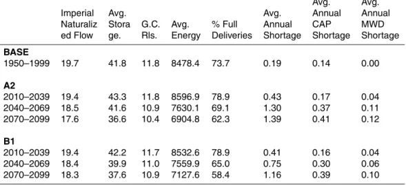
Table 4. Streamflow at Imperial Dam, AZ (BCM/yr), average 1 January total basin storage

(BCM), release from Glen Canyon Dam (BCM/yr), annual energy production (GW-h/yr), per-centage of years with no delivery shortages, average annual delivery shortage (BCM/yr), av-erage annual CAP delivery shortage (BCM/yr), and annual avav-erage MWD delivery shortage (BCM/yr).

Avg. Avg.

Imperial Avg. Avg. Annual Annual

Naturaliz Stora G.C. Avg. % Full Annual CAP MWD

ed Flow ge. Rls. Energy Deliveries Shortage Shortage Shortage

BASE 1950–1999 19.7 41.8 11.8 8478.4 73.7 0.19 0.14 0.00 A2 2010–2039 19.4 43.3 11.8 8596.9 78.9 0.43 0.17 0.04 2040–2069 18.5 41.6 10.9 7630.1 69.1 1.30 0.37 0.11 2070–2099 17.6 36.6 10.4 6904.8 62.3 1.39 0.41 0.12 B1 2010–2039 19.4 42.2 11.7 8532.6 78.9 0.41 0.16 0.04 2040–2069 18.4 39.9 11.0 7559.9 65.0 0.75 0.30 0.06 2070–2099 18.3 37.6 10.9 7127.6 58.4 1.16 0.39 0.10 3756

(32)

HESSD

3, 3727–3770, 2006

Full Screen / Esc

(33)

HESSD

3, 3727–3770, 2006

Full Screen / Esc

Printer-friendly Version Interactive Discussion 0 5 10 15 20 25 30 35 1905 1915 1925 1935 1945 1955 1965 1975 1985 1995 2005 A n n u a l F lo w ( B C M )