HAL Id: hal-00318004
https://hal.archives-ouvertes.fr/hal-00318004
Submitted on 19 May 2006
HAL is a multi-disciplinary open access
archive for the deposit and dissemination of
sci-entific research documents, whether they are
pub-lished or not. The documents may come from
teaching and research institutions in France or
abroad, or from public or private research centers.
L’archive ouverte pluridisciplinaire HAL, est
destinée au dépôt et à la diffusion de documents
scientifiques de niveau recherche, publiés ou non,
émanant des établissements d’enseignement et de
recherche français ou étrangers, des laboratoires
publics ou privés.
A modeling study of ionospheric F2-region storm effects
at low geomagnetic latitudes during 17-22 March 1990
A. V. Pavlov, S. Fukao, S. Kawamura
To cite this version:
A. V. Pavlov, S. Fukao, S. Kawamura. A modeling study of ionospheric F2-region storm effects at low
geomagnetic latitudes during 17-22 March 1990. Annales Geophysicae, European Geosciences Union,
2006, 24 (3), pp.915-940. �hal-00318004�
Ann. Geophys., 24, 915–940, 2006 www.ann-geophys.net/24/915/2006/ © European Geosciences Union 2006
Annales
Geophysicae
A modeling study of ionospheric F2-region storm effects at low
geomagnetic latitudes during 17–22 March 1990
A. V. Pavlov1, S. Fukao2, and S. Kawamura3
1Pushkov Institute of Terrestrial Magnetism, Ionosphere and Radio-Wave Propagation, Russian Academy of Science (IZMIRAN), Troitsk, Moscow Region, 142190, Russia
2Research Institute for Sustainable Humanosphere (RISH), Kyoto University, Kyoto, 611-0011, Japan
3National Institute of Information and Communications Technology, 4-2-1, Nukui-kita, Koganei, Tokyo 184-8795, Japan
Received: 6 September 2005 – Revised: 9 March 2006 – Accepted: 23 March 2006 – Published: 19 May 2006
Abstract. We have presented a comparison between the modeled NmF2 and hmF2, and NmF2 and hmF2, which were observed in the low-latitude ionosphere simultaneously by the Kokubunji, Yamagawa, Okinawa, Manila, Vanimo, and Darwin ionospheric sounders, by the middle and upper at-mosphere (MU) radar during 17–22 March 1990, and by the Arecibo radar for the time period of 20–22 March 1990. A comparison between the electron and ion temperatures mea-sured by the MU and Arecibo radars and those produced by the model of the ionosphere and plasmasphere is pre-sented. The empirical zonal electric field, the meridional neutral wind taken from the HWM90 wind model, and the NRLMSISE-00 neutral temperature and densities are cor-rected so that the model results agree reasonably with the ionospheric sounder observations, and the MU and Arecibo radar data. It is proved that the nighttime weakening of the equatorial zonal electric field (in comparison with that pro-duced by the empirical model of Fejer and Scherliess (1997) or Scherliess and Fejer (1999)), in combination with the cor-rected wind-induced plasma drift along magnetic field lines, provides the development of the nighttime enhancements in NmF2 observed over Manila during 17–22 March 1990. As a result, the new physical mechanism of the nighttime NmF2 enhancement formation close to the geomagnetic equator in-cludes the nighttime weakening of the equatorial zonal elec-tric field and equatorward nighttime plasma drift along mag-netic field lines caused by neutral wind in the both geomag-netic hemispheres. It is found that the latitudinal positions of the crests depend on the E×B drift velocity and on the neutral wind velocity. The relative role of the main mecha-nisms of the equatorial anomaly suppression observed dur-ing geomagnetic storms is studied for the first time in terms of storm-time variations of the model crest-to-trough ratios of the equatorial anomaly. During most of the studied time Correspondence to: A. V. Pavlov
(pavlov@izmiran.rssi.ru)
period, a total contribution from meridional neutral winds and variations in the zonal electric field to the equatorial anomaly changes is larger than that from geomagnetic storm disturbances in the neutral temperature and densities. Vibra-tionally excited N2and O2promote the equatorial anomaly enhancement during the predominant part of the studied time period, however, the role of vibrationally excited N2and O2 in the development of the equatorial anomaly is not signifi-cant. The asymmetries in the neutral wind and densities rela-tive to the geomagnetic equator are responsible for the north-south asymmetry in NmF2 and hmF2, and for the asymmetry between the values of the crest-to-trough ratios of the North-ern and SouthNorth-ern Hemispheres. The model simulations pro-vide epro-vidence in favor of an asymmetry in longitude of the energy input into the auroral region of the Northern Hemi-sphere on 21 March 1990.
Keywords. Ionosphere (Electric fields and currents; Equato-rial ionosphere; Plasma temperature and density; Ionospheric disturbances; Modeling and forecasting)
1 Introduction
Geomagnetic storm effects on the ionosphere depend on sea-son, latitude, and longitude, as well as on the severity, time of occurrence, and duration of the storm, and the geomagnetic storm changes in electric fields, thermospheric winds and neutral composition have been suggested to explain varia-tions in the low-latitude ionosphere (Abdu et al., 1991; Abdu, 1997; Buonsanto, 1999; Rishbeth, 1975, 2000; Pavlov et al., 2004b and references therein). The storm-time F-region changes at low geomagnetic latitudes have been identified from F-layer height and frequency responses observed by ionosondes (see Abdu, 1997 and references therein). The dynamics of the low-latitude ionosphere was observed by the middle and upper atmosphere (MU) radar during the
916 A. V. Pavlov et al.: A modeling study of ionospheric F2-region storm effects geomagnetic storms of 6–8 February 1986, 20–21 January
1989, 20–23 October 1989, and 25–27 August 1987 (Oliver et al., 1988; Reddy et al., 1990; Oliver et al., 1991; Pavlov et al., 2004b). The changes in F-layer electron density ob-served by the MU radar in the 6–8 February 1986 storm were explained by changes in an influx of ionization from the plasmasphere, modulated by the passage of a large-scale, southward traveling gravity wave (Oliver et al., 1988). In the 20–21 January 1989 storm, the observed large changes in the F2-region peak altitude from 23:00 LT to 02:40 LT were attributed to a large eastward electric field originat-ing at auroral latitudes (Reddy et al., 1990). Duroriginat-ing the 20–23 October 1989 storm-time period, drastically different electron densities were discovered in the F-region (Oliver et al., 1991). Pavlov et al. (2004b) have presented a compari-son of the modeled F2-layer peak densities, NmF2, and al-titudes, hmF2, with NmF2 and hmF2, which were observed at low geomagnetic latitudes simultaneously by the Akita, Kokubunji, Yamagawa, Okinawa, Manila, Vanimo, and Dar-win ionospheric sounders and by the MU radar during the 25–27 August 1987 geomagnetically storm, taking into ac-count the storm-time changes in the thermospheric wind, the electric field, the neutral composition, and the neutral tem-perature. It is found by Pavlov et al. (2004b) that the geo-magnetic latitude variations in NmF2, calculated for 26 Au-gust 1987 (the recovery phase of the geomagnetic storm), differ significantly from those calculated for 25 August 1987 (before SSC and during the main phase of the geomagnetic storm) and for 27 August 1987 (after the geomagnetic storm). The Arecibo radar observations of the ionospheric F-region during the 1–5 May 1995 geomagnetic storm period have shown that there is the possibility of poleward expansion of the equatorial anomaly zone with the northern anomaly crest location close to the 29◦dip latitude (Buonsanto, 1999). Another anomalous low-latitude ionospheric feature was ob-served during the 17–18 February 1999 highly disturbed geo-magnetic period, when the Arecibo radar recorded an anoma-lous nighttime ionospheric enhancement in which the night-time value of NmF2 exceeded 106cm−3and the F2 peak al-titude went above 400 km (Aponte et al., 2000).
The effects of geomagnetic storms on the low-latitude ionosphere and plasmasphere have attracted much inter-est. The simplified theoretical computations of Burge et al. (1973) and Chandra and Spencer (1976) have speculated on the importance of the disturbed neutral winds to the low-latitude ionospheric response to geomagnetic storms, but lack of data and/or model winds has hampered progress. Ig-noring electric field perturbations, due to the storm during 22 March 1979, and suggesting that the temperatures of elec-trons and ions are equal to the neutral temperature, Fesen et al. (1989) found that the equatorial anomaly may be dis-rupted by the magnetic storms, and that the major factor in-fluencing the storm-time ionospheric behavior is the neutral wind. Variations in the low-latitude ionosphere for a hypo-thetical geomagnetic storm at equinox and high solar activity
were studied by Fuller-Rowell et al. (2002), without taking into account geomagnetic storm disturbances in the electric field. Their model results made clear the difference between the effects of meridional and zonal winds on the disturbed ionosphere.
Electric fields E affect the distribution of plasma in the low-latitude ionospheric F-region, causing both ions and electrons to drift in the same direction with a drift veloc-ity, VE=E×B/B2, perpendicular to the geomagnetic field B direction. The present work studies the relationship be-tween variations in the meridional component of VE and the dynamics of the low-latitude F2-layer in the low-latitude ionosphere, when NmF2 and hmF2 are observed simultane-ously by the Kokubunji, Yamagawa, Okinawa, Manila, Van-imo, and Darwin ionospheric sounders and by the MU and Arecibo radars during the 17–22 March 1990 geomagneti-cally storm-time period. We investigate how well the mea-sured electron density and temperature at Arecibo and Shi-garaki, and NmF2 and hmF2, observed by the ionospheric sounders agree with those generated by the 2-D time depen-dent model of the low-and middle-latitude ionosphere and plasmasphere of Pavlov (2003).
If the E×B plasma drift is directed from lower L-shells to higher L-shells, then a decrease in the E×B plasma drift leads to decreases in NmF2 in the crest regions and to an in-crease in NmF2 in the trough region, hampering the equa-torial anomaly development, while a strengthening of this plasma drift causes an equatorial anomaly enhancement. A plasma drift due to wind transports plasma along magnetic field lines and causes changes in NmF2 and in the crest-to-trough ratio of NmF2 in the Northern and Southern Hemi-spheres, leading to a weakening or a strengthening of the equatorial anomaly. The value of NmF2 is a function of [O], [N2], and [O2] at hmF2 at low geomagnetic latitudes (e.g. Pavlov et al., 2004b), and, therefore, storm-time changes in these number densities in one of the crest regions or in both crest regions or in the trough region contribute to changes in the equatorial anomaly development. As far as the authors know, the relative role of these mechanisms in the equatorial anomaly suppression is studied only by Pavlov et al. (2004b) for the 25–26 August 1987 geomagnetic storm. Pavlov et al. (2004b) found that weak differences between disturbed and quiet E×B plasma drifts cannot be responsible for the suppression of the equatorial anomaly on 26 August, and this suppression is due to the action of storm-time changes in neutral winds and densities on the equatorial anomaly de-velopment.
In this paper, we continue the study of the complex prob-lem of the low-latitude ionospheric response to variations in the thermospheric wind, electric field, neutral composition, and neutral temperature during 17–22 March 1990 at solar maximum in the present case study, in which the electron density and temperature are measured simultaneously by the MU and Arecibo radars, and NmF2 and hmF2 are observed by the Kokubunji, Yamagawa, Okinawa, Manila, Vanimo,
A. V. Pavlov et al.: A modeling study of ionospheric F2-region storm effects 917 and Darwin ionospheric sounders. The use of data from the
MU radar and the Arecibo radar, in combination with the ionosonde measurements, allows us to investigate the differ-ences and similarities between the storm effects in the iono-sphere in the different longitude sectors at low geomagnetic latitudes.
It has been well established that the F2-peak electron den-sity shows anomalous nighttime enhancements under various geophysical conditions (see Pavlov and Pavlova, 2005a, and references therein). Many theories have been put forward to explain these nighttime enhancements in NmF2. The mech-anism which can account for the observed nighttime NmF2 enhancements at middle geomagnetic latitudes is a combina-tion of the plasmaspheric heating and refilling, and chemical and plasma transport effects (Pavlov and Pavlova, 2005a). The observed features of the nighttime enhancements in the total ionospheric electron content, TEC, at low geomagnetic latitudes, were reported by various workers (e.g. Young et al., 1970; Nelson and Cogger, 1971; Lanzerotti et al., 1975; Tyagi et al., 1982; Balan et al., 1994; Su et al., 1994; Jain et al., 1995; Unnikrishnan et al., 2002). The post-sunset en-hancements in TEC and NmF2 of the low-latitude ionosphere during geomagnetically quiet conditions were studied by An-derson and Klobuchar (1983), Dasgupta et al. (1985), Balan et al. (1995), and Su et al. (1995, 1997), using theoretical modeling techniques. Anderson and Klobuchar (1983) and Dasgupta et al. (1985) have shown that the prereversal in-crease of the meridional component of the E×B drift velocity primarily determines the development of the post-sunset en-hancements in TEC near the crests of the equatorial anomaly. Seasonal, solar activity and latitude variations of the post-sunset enhancements in TEC and NmF2 in the 10–30◦ ge-omagnetic latitude range at longitude 158◦W were studied by Balan et al. (1995). The model calculations of Su et al. (1995), carried out for July at solar maximum, confirmed that the primary source for the nighttime enhancement in TEC at geomagnetic latitude 19◦is the prereversal increase in the E×B plasma drift. It is shown by Su et al. (1997) that the difference in time of occurrence between the peak value of the prereversal increase in the E×B plasma drift and in the peak values of TEC and NmF2 at equinox under solar maxi-mum conditions at the crests of the equatorial anomaly varies with longitude because of the longitudinal difference of the neutral wind.
In this paper, we present the first theoretical study of the physical mechanisms responsible for electron density en-hancements at night close to the geomagnetic equator, us-ing the sounder low-latitude data durus-ing 17–22 March 1990 and a time-dependent two-dimensional model of the low-and middle-latitude ionosphere low-and plasmasphere described in Sect. 2.
O+(4S) ions which dominate at ionospheric F2-region al-titudes are lost in the reactions of O+(4S) with unexcited N2(v=0) and O2(v=0) and vibrationally excited N2(v) and O2(v) molecules at vibrational levels, v>0. Vibrationally
excited N2 and O2 react more strongly with O+(4S) ions in comparison with unexcited N2 and O2 (Schmeltekopf et al., 1968; Hierl et al., 1997). As a result, an additional re-duction in the electron density is caused by the reactions of O+(4S) ions with vibrationally excited N2 and O2 (Pavlov, 1994; Richards et al., 1994b; Jenkins et al., 1997; Pavlov and Buonsanto, 1997; Pavlov and Oyama, 2000; Pavlov and Fos-ter, 2001; Pavlov, 2003; Pavlov et al., 2004a, b). In this paper we examine the effects of vibrationally excited N2 and O2 on the electron density and temperature during 17–22 March 1990 and study, for the first time, the role of N2(v>0) and O2(v>0) in the equatorial anomaly development.
2 Theoretical model
The model of the low- and middle-latitude ionosphere and plasmasphere, which is described in detail by Pavlov (2003), calculates number densities, Ni, of O+(4S), H+, NO+, O+2, N+2, O+(2D), O+(2P), O+(4P), and O+(2P*) ions, the elec-tron density, Ne, and temperature, Te, and the ion tem-perature, Ti. The model includes the production and loss rates of ions by the photochemical reactions presented by Pavlov (2003) and Pavlov and Pavlova (2005b), except for the rate coefficient of the O+(2D)+O reaction, which is taken from Fox and Dalgarno (1985). The horizontal components of the neutral wind are specified using the HWM90 wind model (Hedin et al., 1991); the model solar EUV fluxes are produced by the EUVAC model (Richards et al., 1994a), while neutral densities and temperature are taken from the NRLMSISE-00 model (Picone et al., 2002).
The model calculations are carried out in dipole orthogo-nal curvilinear coordinates q, U, and 3, where q is aligned with, and U and 3 are perpendicular to, B, and the U and 3 coordinates are constant along a dipole magnetic field line. It should be noted that q=(RE/R)2 cos 2, U=(RE/R) sin2
2, and the value of 3 is the geomagnetic longitude, where R is the radial distance from the geomagnetic field center,
2=900−ϕ is the geomagnetic colatitude, ϕ is the geomag-netic latitude, RE is the Earth’s radius.
The model takes into account that the E×B plasma drift velocity can be presented as VE=VE
3 e3+V E
U eU, where VE3= EU/B is the zonal component of VE, VEU=–E3/B is the meridional component of VE, E=E3e3+EU eU , E3 is the
3(zonal) electric field in the dipole coordinate system, EU is the U (meridional) component of E in the dipole coordi-nate system, e3 and eU are unit vectors in 3 and U direc-tions, respectively, eU is directed downward at the geomag-netic equator. We use the implementation of the Eulerian-Lagrangian method developed by Pavlov (2003) in solving the time dependent and two-dimensional continuity and en-ergy equations at a (q,U) plane. The combination of the Lagrangian and Euleurean approaches used consists mainly of two steps, an advection step and an interpolation step (Pavlov, 2003). The trajectory of the ionospheric plasma
918 A. V. Pavlov et al.: A modeling study of ionospheric F2-region storm effects
Table 1. Ionosonde station and radar names and locations. Geomagnetic latitudes and longitudes of the ionosonde stations and radars are
calculated on the surface of the Earth in the eccentric (first number) and centered (second number) dipole approximations for the geomagnetic field using the parameters of these magnetic field approximations for the time period 1990. The calculated L-shell values correspond to magnetic field lines which intersect 300-km altitude over the sounders and radars, the eccentric (first number) and centered (second number) dipole approximations are used.
Ionosonde station Geographic Geographic Geomagnetic Geomagnetic L and radar names latitude longitude latitude longitude
Kokubunji 35.7 139.5 27.4, 26.2 206.7, 207.5 1.228, 1.300 Yamagawa 31.2 130.6 21.7, 21.0 198.5, 199.8 1.124, 1.202 Okinawa 26.3 127.8 16.2, 16.0 196.1, 197.6 1.052, 1.133 Manila 14.6 121.1 3.2, 4.0 189.9, 191.9 0.977, 1.052 Vanimo –2.7 141.3 –13.9, –11.8 213.0, 213.2 1.033, 1.093 Darwin –12.45 130.95 –25.3, –22.5 202.3, 203.4 1.199, 1.226 MU radar 34.85 136.10 26.1, 25.1 203.5, 204.5 1.202, 1.276 Arecibo radar 18.35 293.25 26.5, 29.2 7.2, 4.8 1.377, 1.373
perpendicular to magnetic field lines and the moving co-ordinate system are determined from equations derived by Pavlov (2003). The effects of the zonal (geomagnetic east-geomagnetic west) component of the E×B drift on Ne, Ni, Te, and Ti are not taken into consideration because it is be-lieved (Anderson, 1981) that these effects are negligible. As a result, the model works as a time dependent, 2-D (q and U coordinates) model of the ionosphere and plasmasphere. In this approximation, time variations of U, caused by the exis-tence of the zonal electric field, are determined by time vari-ations of the effective zonal electric field, Eeff3=E3RR−1E sin
2, and the value of Eeff3 is not changed along a magnetic field line (Pavlov, 2003).
Pavlov (2003) and Pavlov et al. (2004 a, b) used a math-ematical model of the ionosphere and plasmasphere which incorporated a centered tilted magnetic dipole representation for the geomagnetic field and employed the averaged param-eters (Akasofu and Chapman, 1972) of the centered tilted magnetic dipole, whose magnetic moment is located in the Earth’s center and is inclined with respect to the Earth’s ro-tational axis (the first three coefficients in the expansion of the geomagnetic field potential are taken into consideration in this approach). In the updated model of the ionosphere and plasmasphere, the Earth’s magnetic field is approximated by the field of the eccentric tilted magnetic dipole, whose mag-netic moment is inclined with respect to the Earth’s rotational axis but is located at a point which is not coincided with the Earth’s center (the first eight nonzero coefficients in the ex-pansion of the geomagnetic field potential in terms of spher-ical harmonics are taken into account). The dependences of the parameters of the eccentric tilted magnetic dipole on a year are given by Frazer-Smith (1987) and Deminov and Fishchuk (2000).
The model calculates the values of Ni, Ne, Ti, and Te in the fixed nodes of the fixed volume grid. This Eulerian
computational grid consists of a distribution of the dipole magnetic field lines in the ionosphere and plasmasphere. One hundred dipole magnetic field lines are used in the model for each fixed value of 3. The number of the fixed nodes taken along each magnetic field line is 191. For each fixed value of 3, the region of study is a (q, U) plane, which is bounded by two dipole magnetic field lines. The computa-tional grid dipole magnetic field lines are distributed between the low and upper boundary lines. Each computational grid dipole magnetic field line intersects the geomagnetic equato-rial point (q=0) at the geomagnetic equatoequato-rial crossing height hkeq=h1eq+1h1eq+. . . +1hkkeq, where k=1,. . . kk, kk=100, 1hkeq is the interval between neighboring computational grid lines. In the model, the low boundary magnetic field line intersects the geomagnetic equatorial point at the geomagnetic equa-torial crossing height h1eq=150 km. The computational grid lines have the interval 1hkeq of 20 km for k=1 and 2, and the value of 1hkeqis increased from 20 km to 42 km linearly, if the value of k is changed from k=2 to k=kk. The upper boundary magnetic field line has hkk
eq=4264 km.
In this work, we use data from the MU and Arecibo radars and from the Kokubunji, Yamagawa, Okinawa, Manila, Van-imo, and Darwin ionospheric sounders (see Sect. 3), whose locations are shown in Table 1. It follows from Table 1 that the sounders and the MU radar are located within ±11.55◦ geomagnetic longitude of one another, if the eccentric tilted magnetic dipole representation for the geomagnetic field is used. As a result, the model simulations are carried out in the (q, U) plane of 201.45◦geomagnetic longitude, to compare the model results with the MU radar and sounder measure-ments. If the eccentric tilted magnetic dipole approximation for the geomagnetic field is applied, then the Arecibo radar is located in the (q, U) plane of 7.2◦geomagnetic longitude, where the model simulations are carried out separately. If the geomagnetic field is represented by the eccentric tilted
A. V. Pavlov et al.: A modeling study of ionospheric F2-region storm effects 919 0 12 0 12 0 12 0 12 0 12 0 12 24 UT (hours) Fig. 1 0 1 2 3 4 5 6 7 Kp -120 -100 -80 -60 -40 -20 0 20 Ds t ( γ) 17-22 March 1990 0 200 400 600 800 1000 1200 AE ( n T) SSC 37
Fig. 1. The variation in the AE index (top panel), the Dst index (middle panel), and Kp index (bottom panel) during 17–22 March 1990. The
SSC onset of the second geomagnetic storm is shown by the arrow in the bottom panel.
magnetic dipole, then the L-shell value of the upper bound-ary magnetic field line is equal to 1.592 and 1.738 for the (q, U) plane of 201.45◦geomagnetic longitude and for the Arecibo (q, U) plane, respectively.
The empirical model of the storm-time vertical drift ve-locity of Fejer and Scherliess (1997) is used to determine Eeff3 at the equatorial dipole magnetic field lines which in-tersect the geomagnetic equatorial points at the geomagnetic equatorial crossing heights hkeq ≤600 km. The value of E3, which corresponds to the plasma drift velocity, is corrected in order to bring the measured and modelled F2-region peak al-titudes into better agreement (see Sect. 4.1.1). This corrected equatorial zonal electric field is considered as the disturbed equatorial zonal electric field for the studied time period.
There are no MU radar vertical drift velocity measure-ments for the period under investigation. We take into ac-count that the perpendicular drifts over Arecibo and the MU radar are similar for the same local time (Takami et al., 1996). Let us us LAas the McIlwain parameter of the geomagnetic field line, which corresponds to the Arecibo radar. The av-erage time zonal electric field derived from Arecibo radar scatter observations, appropriate for a high level of solar ac-tivity, is determined from the corresponding average E×B drift given by Fig. 2 of Fejer (1993). In the absence of mea-surements and an empirical model of a zonal electric field for the studied time period at F2-region altitudes for mag-netic field lines which correspond to L>LA, we suggest that the value of the effective zonal electric field is not changed at
920 A. V. Pavlov et al.: A modeling study of ionospheric F2-region storm effects 300-km altitude for magnetic field lines at L≥LA. The
effec-tive equatorial zonal electric field is assumed to be the same at the geomagnetic equator for equatorial magnetic field lines with hkeq<600 km. A linear interpolation between the equa-torial and Arecibo values of the effective zonal electric field is employed at intermediate dipole magnetic field lines. The value of the zonal electric field is corrected to make the mea-sured and modeled F2-region peak altitudes agree during the studied time period (see Sect. 4).
In the (q, U) plane of 201.45◦geomagnetic longitude, the model starts at 05:13 UT on 15 March. This UT corresponds to 14:00 SLT (solar local time) at the geomagnetic equator and 201.45◦of the geomagnetic longitude (SLT=UT+ψ /15, where ψ is the geographic latitude). The model is run from 05:13 UT on 15 March 1990 to 24:00 UT on 16 March 1990 before model results are used. The model starts at 18:24 UT on 17 March in the Arecibo (q, U) plane. This UT corre-sponds to 14:00 SLT at the geomagnetic equator and 7.2◦of the geomagnetic longitude. The model is run from 18:24 UT on 17 March 1990 to 24:00 UT on 19 March 1990 before model results are used. We expect our finite-difference al-gorithm, which is described below, to yield approximations to Ni, Ne, Ti, and Tein the ionosphere and plasmasphere at discrete times t=0, 1t, 21t, and so on up to the final discrete time with the time step 1t=10 min.
3 Solar geophysical conditions and data
The geomagnetically quiet conditions of 17 March 1990 (the geomagnetic activity index Ap changes from 3 to 8) and the 18–22 March 1990 magnetic storm period (the value of Ap changes from 14 to 73) were periods which occurred at solar maximum, when the 10.7 solar flux varied between 182 on 17 March and 243 on 22 March. In Fig. 1, the geomagnetic activity indexes Kp (bottom panel), Dst (middle panel), and AE (top panel), taken by INTERNET from the database of the National Geophysical Data Center (Boulder, Colorado, are plotted versus universal time. It is seen from Fig. 1 that during the 18–22 March 1990 period two geomagnetic storms took place with a gradual commencement time near 04:00 UT on 18 March and with a sudden commencement time near 22:45 UT on 20 March.
Intense storms have minimum values of Dst≤–100 nT (Gonzalez and Tsurutani, 1987), while the first studied storm reached the minimum value of Dst=–67 nT at 01:00 UT– 02:00 UT on 19 March 1990, followed by the recovery phase of the storm. Thus, this storm can be classified as a moderate storm. The AE index of the first storm remained perturbed until about 02:50–03:00 UT on 19 March. The SSC onset of the second geomagnetic storm was at 22:43 UT on 21 March and is shown by the arrow in the bottom panel of Fig. 1. This storm has the minimum value of Dst=–136 nT at 06:00 UT– 07:00 UT on 21 March 1990 followed by the recovery phase of the geomagnetic storm, and this storm can be classified as
an intense storm. The Dst index remained at less than –60 nT from 00:00 UT on 21 March to 24:00 UT on 22 March. The Kp index reached its maximum value of 6− at 15:00 UT– 18:00 UT and on 18 March and at 00:00 UT–03:00 UT on 19 March during the moderate storm, while the Kp maximum value was 7+at 00:00 UT–03:00 UT on 22 March during the intense storm.
The MU radar operated from 11:52 LT on 19 March to 11:37 LT on 22 March. The capabilities of the radar for in-coherent scatter observations have been described and com-pared with those of other incoherent scatter radars by Sato et al. (1989) and Fukao et al. (1990). Rishbeth and Fukao (1995) reviewed the MU radar studies of the ionosphere and thermosphere. The data that we use in this work are the measured time variations of altitude profiles of the electron density and temperature, and the ion temperature between 200 km and 600 km over the MU radar.
The Arecibo incoherent scatter radar operated during the period 14:29 UT on 19 March to 02:00 UT on 23 March 1990, obtaining data on electron density, and electron and ion temperature variations. The experimental sequences used contained a number of pointing directions, but this study will use data observed in a local mode, using a scan at elevation angles between 75 and 90◦. The final anal-ysed data set covers the 145 to 686-km altitude with ap-proximately 37–38-km resolution. Data are accessed using the MADRIGAL database at the Millstone Hill Observatory website (http://www.haystack.mit.edu/madrigal), located at Massachusetts Institute of Technology’s Haystack Observa-tory. The detailed description of the Arecibo radar experi-ment is given by Buonsanto et al. (1992) and Buonsanto and Foster (1993).
We use hourly critical frequencies, fof2 and foE, of the F2 and E-layers, and maximum usable frequency parameter, M(3000)F2, data from the Manila ionospheric sounder sta-tion available at the Ionospheric Digital Database of the Na-tional Geophysical Data Center, Boulder, Colorado. Hourly fof2, M(3000)F2, and foE ionospheric parameters measured by the Kokubunji, Yamagawa, and Okinawa sounders were obtained from the National Institute of Information and Com-munications Technology of Japan, while the Australian Gov-ernment IPS Radio and Space Service was used to obtain these data by Internet for the Vanimo and Darwin ionoson-des.
The locations of these ionospheric sounder stations and the location of the MU and Arecibo radars are shown in Ta-ble 1. The value of the peak density, NmF2, of the F2 layer is related to the critical frequency fof2 as NmF2=1.24·1010 fof22, where the unit of NmF2 is m−3, the unit of fof2 is MHz. In the absence of adequate hmF2 data, we use the re-lation between hmF2 and the values of M(3000)F2, fof2, and foE recommended by Dudeney (1983) from the comparison of different approaches as hmF2=1490/[M(3000)F2+1M]– 176, where 1M=0.253/(fof2/foE–1.215)–0.012. If there are no foE data, then it is suggested that 1M=0, i.e. the hmF2
A. V. Pavlov et al.: A modeling study of ionospheric F2-region storm effects 921 formula of Shimazaki (1955) is used. The reliability of hmF2
derived from the observed values of M(3000)F2, fof2, and foE by means of the Dudeney (1983) approach is also sup-ported by the reasonable agreement between these values of hmF2 and those measured by the MU radar during the geo-magnetically quiet conditions of 19–21 March 1988 (Pavlov et al., 2004a), and during the geomagnetic storm periods of 25–27 August 1987 (Pavlov et al., 2004b) and 19–22 March 1990 (see Fig. 6, which is explained in Sect. 4.1.1).
4 Model results and discussion
4.1 The (q, U) plane at geomagnetic longitude 201.45◦ 4.1.1 Model/data comparisons
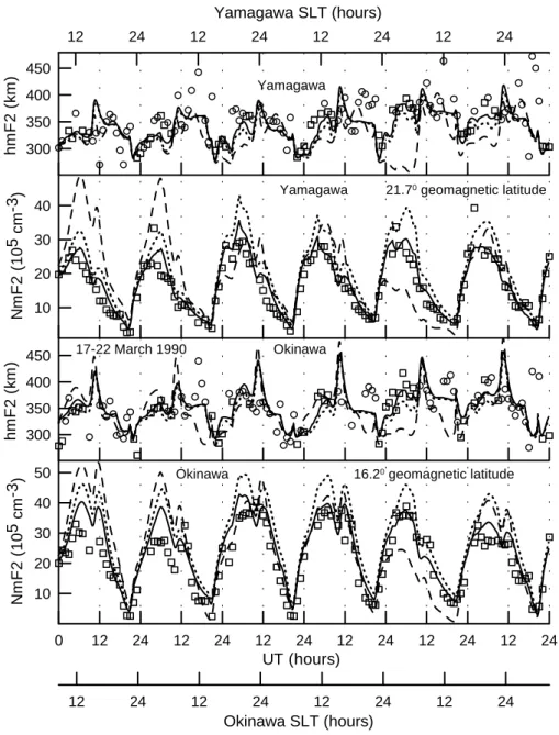
The measured (squares and circles) and calculated (lines) NmF2 and hmF2 are displayed in Figs. 3–5 for the period under investigation above the Darwin (two lower panels in Fig. 3), Vanimo (two upper panels in Fig. 3), Manila (Fig. 4), Okinawa (two lower panels in Fig. 5), and Yamagawa (two upper panels in Fig. 5) ionosonde stations. The two lower panels of Fig. 6 show NmF2 and hmF2 measured by the Kokubunji ionosonde station (squares and circles) and MU radar (crosses), in comparison with the calculated (lines) NmF2 and hmF2 over the MU radar, while the measured (crosses) and modeled (lines) electron and O+ion tempera-tures at the F2-region main peak altitude above the MU radar are presented in the two upper panels of Fig. 6. The rela-tions between hmF2 and the values of M(3000)F2, fof2, and foE (see Sect. 3) are used to determine the values of hmF2 shown by squares and circles, when the measured values of foE are acceptable and not acceptable, respectively, i.e. the magnitudes of hmF2 shown by circles in Figs. 3–6 are overestimated. The results obtained from the model using the combination of Eeff3, based on the uncorrected zonal dis-turbed equatorial electric field (given by the dashed line in the bottom panel of Fig. 2), the NRLMSISE-00 neutral tem-perature and densities, and the HWM90 wind, as the input model parameters, are shown by dashed lines in Figs. 3–6. Solid and dotted lines in Figs. 3–6 show the results given by the model with the corrected zonal equatorial electric field (given by the solid line in the bottom panel of Fig. 2), the corrected NRLMSISE-00 neutral densities, and the cor-rected neutral wind, when vibrationally excited N2(v>0) and O2(v>0) are included (solid lines) and not included (dotted lines) in the loss rate of O+(4S) ions. The corrections of E3 and the NRLMSISE-00 and HWM90 model corrections used in the model simulations, shown by solid and dotted lines in Figs. 3–6, are explained below.
It is seen from the comparison between the correspond-ing solid lines and data in Figs. 3–6 that the use of the cor-rected NRLMSISE-00 neutral densities, the corcor-rected merid-ional HWM90 wind, and the corrected zonal electric field
brings the measured and modeled NmF2, hmF2, Te, and Ti into reasonable agreement, although there are some quan-titative differences. The reasonable agreement between the measured and modeled Te and Ti determines the reliabil-ity of the calculated Te and Ti at other geomagnetic lati-tudes. It should be noted that the measured hmF2 presented in Figs. 3–6 show large fluctuations. The possible source of this scatter in hmF2 is the relationship between hmF2 and M(3000)F2 and 1M (see Sect. 3), which determines hmF2 with errors. Furthermore, the ionosondes listed in Table 1 are not located at the geomagnetic longitude of 201.45◦, which is used in the model calculations. This geomagnetic longi-tude displacement can explain a part of the disagreement be-tween the modeled and measured hmF2, NmF2, Te, and Tiin Figs. 3–6. A part of these discrepancies is probably due to the uncertainties in the model inputs, such as E3, the NRLMSIS-00 model densities and temperature, the neutral wind, EUV fluxes, chemical rate coefficients, and photoionization, pho-toabsorption and electron impact cross sections for N2, O2, and O.
It follows from Figs. 3–6 that the use of the uncorrected E3and the original HWM90 wind and NRLMSISE-00 neu-tral temperature and densities as the input model parameters brings the measured (squares, circles and crosses) and mod-eled (dashed lines) NmF2, hmF2, Te, and Ti into disagree-ment.
The vertical equatorial drift shows significant variability in the magnitude (Fejer, 2002), and the significant day-to-day variability of the quiet plasma drift in events from a database of Jicamarca observations was demonstrated by Scherliess and Fejer (1999). The empirical models of Scherliess and Fejer (1999) and Fejer and Scherliess (1997) for quiet and ge-omagnetically storm-time periods were created by averaging a great deal of data to find the mean trends in noisy data and create smooth curves. As a result, the averaged vertical drifts produced by these empirical models can differ from the ver-tical drifts for the studied time period, and can be modified to bring the measured and modeled NmF2 and hmF2 into rea-sonable agreement over the Manila, Vanimo, and Okinawa sounders.
The time variations of the zonal electric field used in the model calculations are presented in the bottom (geomagnetic equator) and top (Arecibo) panels of Fig. 2. The dashed line in the bottom panel of Fig. 2 shows the empirical F-region storm-time equatorial zonal electric field found from the empirical model of the vertical drift velocity of Fejer and Scherliess (1997). The empirical model of Scherliess and Fejer (1999) is used to determine the F-region geomagneti-cally quiet equatorial zonal electric field shown by the dotted line in the bottom panel of Fig. 2. By the use of the com-parison between the measured and modeled values of hmF2 and NmF2 over the Manila, Vanimo, and Okinawa sounders, the value of this quiet equatorial zonal electric field was de-creased by a factor of 1.5 from 23:00 UT on 16 March to 08:30 UT on 17 March, by a factor of 2 from 8:30 UT to
922 A. V. Pavlov et al.: A modeling study of ionospheric F2-region storm effects 0 12 24 12 24 12 24 12 24 12 24 12 24 UT (hours) Fig. 2 -1.2 -0.9 -0.6 -0.3 0 0.3 0.6 0.9 EΛ (m V m -1) -0.2 0 0.2 0.4 0.6 EΛ (m V m -1) 12 24 12 24 12 24 12 24 12 24 12 24 SLT (hours) 17-22 March 1990 Arecibo Geomagnetic equator 38
Fig. 2. Diurnal variations of the F-region zonal electric field during 17-21 March 1990 over the geomagnetic equator at 201.45◦geomagnetic longitude (bottom panel) and over Arecibo (top panel). The zonal electric field at the F-region altitudes over Arecibo is found from Fig. 2 of Fejer (1993).The dashed line in the bottom panel show the storm-time equatorial zonal electric field found from the empirical model of Fejer and Scherliess (1997), while the geomagnetically quiet equatorial zonal electric field found from the empirical model of Scherliess and Fejer (1999) is presented by the dotted line in the bottom panel. The quiet equatorial zonal electric field is modified by the use of the comparison between the measured and modeled values of hmF2 and NmF2 over the Manila, Vanimo, and Okinawa sounders (see Sect. 4.1) to produce the resulting storm-time equatorial zonal electric field shown by the solid line in the bottom panel. SLT is the local solar time at the geomagnetic equator and 201.45◦geomagnetic longitude on the surface of the Earth.
11:00 UT on 17 March, by a factor of 1.4 from 11:00 UT to 17:00 UT on 17 March, by a factor of 1.6 from 23:00 UT on 17 March to 08:30 UT on 18 March, by a factor of 2 from 8:30 UT to 10:00 UT on 18 March, by a factor of 2 from 07:00 UT to 17:00 UT on 19 March, by a factor of 1.8 from 22:00 UT on 19 March to 07:00 UT on 20 March, by a fac-tor of 1.3 from 07:00 UT to 10:45 UT on 20 March, by a factor of 1.8 from 10:45 UT to 22:00 UT on 20 March, by a factor of 2 from 07:00 UT on 21 March to 07:00 UT on 22 March, by a factor of 1.5 from 07:00 UT to 10:45 UT on 22 March, and by a factor of 2 from 10:45 UT to 17:00 UT on 22 March, to produce the resulting equatorial zonal electric field used in the model simulations and shown by the solid line in the bottom panel of Fig. 2.
As a result of the comparison between the modeled NmF2 and NmF2 measured by the ionosonde stations and by the MU radar, the NRLMSISE-00 model values of [N2] and [O2] were increased by a correction factor of C at all altitudes.
To bring the measured and modeled NmF2 of the North-ern Hemisphere into reasonable agreement, the value of C is found to be 1.5 above 16◦ geomagnetic latitude from 23:00 UT on 16 March to 20:00 UT on 17 March and from 22:00 UT on 17 March to 20:00 UT on 18 March, and its value decreases linearly from 1.5 to 1 in the 16◦geomagnetic latitude range. We found that C=1.6 above 21◦geomagnetic latitude from 03:00 UT to 12:00 UT on 19 March, and the [N2] and [O2] correction factor decreases linearly from 1.6 to 1.4 in the geomagnetic latitude range between 21◦and 0◦. The value of C is estimated from the numerical simulations to be 1.5 and 1.6 at geomagnetic latitudes exceeding 21◦from 04:00 UT to 11:00 UT on 20 March and from 02:00 UT to 10:00 UT on 21 March, respectively, and this correction fac-tor varies linearly from the above-mentioned values to 1 in the geomagnetic latitude range between 21◦and 0◦. In the time period from 21:00 UT on 21 March to 12:00 UT on 22 March, the [N2] and [O2] correction factor is found to
A. V. Pavlov et al.: A modeling study of ionospheric F2-region storm effects 923 0 12 24 12 24 12 24 12 24 12 24 12 24 UT (hours) 10 20 30 Nm F 2 ( 1 0 5 cm -3) 250 300 350 400 450 500 hmF 2 ( k m)
Darwin -25.30 geomagnetic latitude
12 24 12 24 12 24 12 24 12 24 12 24 Darwin SLT (hours) Fig. 3 Darwin 17-22 March 1990 10 20 30 40 Nm F 2 ( 1 0 5 cm -3) 300 350 400 450 500 hm F 2 ( k m)
Vanimo -13.90 geomagnetic latitude
12 24 12 24 12 24 12 24
Vanimo SLT (hours)
Vanimo
39
Fig. 3. Observed (squares and circles) and calculated (lines) NmF2 and hmF2 above the Darwin (two lower panels) and Vanimo (two upper
panels) ionosonde stations during 17–22 March 1990. The relations between hmF2 and the measured values of M(3000)F2, fof2, and foE (see Sect. 3) are used to determine the values of hmF2, when the measured values of foE are acceptable (squares) and not acceptable (circles). The results obtained from the model of the ionosphere and plasmasphere, using Eeff3, based on the uncorrected storm-time zonal electric field given by the dashed line in Fig. 2, the NRLMSISE-00 neutral temperature and densities, and the HWM90 wind as the input model parameters, are shown by the dashed lines. The solid lines show the results obtained from the model of the ionosphere and plasmasphere, using the combinations of Eeff3, based on the corrected zonal electric field given by the solid line in Fig. 2, the corrected NRLMSISE-00 neutral densities, and the corrected neutral wind (see Sect. 4.1.1). The dotted lines show the results from the model with the same values of Eeff3, the HWM90 wind, and the NRLMSISE-00 neutral densities, as for the solid lines, when vibrationally excited N2and O2are not
included in the loss rate of O+(4S) ions.
be 1.3 above 25◦geomagnetic latitude; its value decreases linearly from 1.6 to 1.3 in the 16-25◦ geomagnetic latitude range, and a linear variation in the [N2] and [O2] correction factor from 1 to 1.6 is assumed in the geomagnetic latitude range between 0◦and 16◦.
The reasonable agreement between the measured and modeled NmF2 is found if C=1.5 below –14◦ geomag-netic latitude from 23:00 UT on 16 March to 08:00 UT on 17 March and from 23:00 UT on 17 March to 06:00 UT on 18 March, and its value decreases linearly from 1.5 to 1 if
924 A. V. Pavlov et al.: A modeling study of ionospheric F2-region storm effects 0 12 24 12 24 12 24 12 24 12 24 12 24 UT (hours) Fig. 4 10 20 30 40 Nm F 2 ( 1 0 5 cm -3) 300 400 500 600 hmF2 ( k m)
3.20 geomagnetic latitude Manila 17-22 March 1990
12 24 12 24 12 24 12 24 12 24 12 24
Manila SLT (hours)
40
Fig. 4. Observed (squares and circles) and calculated (lines) NmF2 (bottom panel) and hmF2 (top panel) above the Manila ionosonde station
during 17–22 March 1990. The curves are the same as in Fig. 3.
the geomagnetic latitude is changed from –14◦ to 0◦. The model simulations show that C=1.4 in the Southern Hemi-sphere from 03:00 UT to 12:00 UT on 19 March. In the time period from 00:00 UT to 13:00 UT on 20 March, the [N2] and [O2] correction factor is equal to 1.6 at –14◦ geomag-netic latitude, and its value decreases linearly from 1.6 to 1 if the geomagnetic latitude is changed from –14◦to -25◦and from –14◦to 0◦. The model uses the same value of C in the Southern Hemisphere in the time periods from 20:00 UT on 20 March to 07:00 UT on 21 March and from 22:00 UT on 21 March to 06:00 UT on 22 March. This value of C is found to be 1.2 below –25◦geomagnetic latitude, the [N
2] and [O2] correction factor is evaluated to be 1.4 at –14◦geomagnetic latitude, and the value of C varies linearly from 1 to 1.4 and from 1.4 to 1.2 if the geomagnetic latitude is changed from 0◦to –14◦and from –14◦to –25◦, respectively.
Effects of the E×B plasma drift on hmF2 and NmF2 over the Kokubunji and Darwin sounders and over the MU radar, whose locations are far enough from the geomagnetic equa-tor, are much less than those caused by the plasma drift along magnetic field lines due to the neutral wind (Rishbeth, 2000; Souza et al., 2000; Pincheira et al., 2002; Pavlov, 2003; Pavlov et al., 2004a, b), and variations of hmF2 are predom-inantly determined by variations in the thermospheric wind over these sounders and the MU radar. The HWM90 wind velocities are known to differ from observations (Titheridge, 1995; Kawamura et al., 2000; Emmert et al., 2001; Fejer et al., 2002). The meridional, W, and the zonal components of
the neutral wind are produced by the HWM90 wind model of Hedin et al. (1991) in geographical frame of reference, so that the meridional wind is directed northward for W>0 and southward for W<0. To bring the modeled and mea-sured hmF2 and NmF2 into reasonable agreement over the sounders shown in Table 1 and over the MU radar, the value of W taken from the HWM90 wind model is changed to W+1W. The value of 1W shown in the Fig. 7 by the solid line is used above the geomagnetic latitude of 25◦during 17– 18 March and above the geomagnetic latitude of 21◦during 19–22 March. The dashed line in Fig. 7 is the value of 1W below the geomagnetic latitude of –14◦, while 1W=0 at the geomagnetic equator. A square interpolation of 1W is em-ployed between –14◦and 0◦, between 25◦ and 0◦, and be-tween 21◦and 0◦of the geomagnetic latitude, respectively. 4.1.2 Mechanism of nighttime enhancements in NmF2
close to the geomagnetic equator
The most striking feature of the diurnal variations of the measured NmF2 over Manila, shown in the bottom panel of Fig. 4, is the existence of the observed nighttime enhance-ments. Variations in neutral densities and temperature cannot be responsible for the enhanced ionization in the evening and night hours. Anomalous nighttime increases in NmF2 cannot be explained in terms of traveling ionospheric disturbances, since these disturbances would have to be extremely large to produce the nighttime electron density observed (Young et
A. V. Pavlov et al.: A modeling study of ionospheric F2-region storm effects 925 0 12 24 12 24 12 24 12 24 12 24 12 24 UT (hours) 10 20 30 40 50 Nm F 2 ( 1 0 5 cm -3) 300 350 400 450 hm F 2 ( k m)
Okinawa 16.20 geomagnetic latitude
12 24 12 24 12 24 12 24 Okinawa SLT (hours) Fig. 5 17-22 March 1990 Okinawa 10 20 30 40 Nm F 2 ( 1 0 5 cm -3 ) 300 350 400 450 hm F 2 ( k m)
Yamagawa 21.70 geomagnetic latitude
12 24 12 24 12 24 12 24
Yamagawa SLT (hours)
Yamagawa
41
Fig. 5. Observed (squares and circles) and calculated (lines) NmF2 and hmF2 above the Okinawa (two lower panels) and Yamagawa (two
upper panels) ionosonde stations during 17–22 March 1990. The curves are the same as in Fig. 3.
al., 1970). The observed nighttime increases of NmF2 can be explained by two mechanisms, first by an additional ion-ization process, and secondly by an influx of ions and elec-trons into the F2-region. At low geomagnetic latitudes, sig-nificant ionization of neutral components of the upper atmo-sphere by energetic particle is rather questionable. It is ev-ident that the anomalous nighttime increases in NmF2 ob-served over Manila during the geomagnetic quiet-time pe-riod of 17 March cannot be explained by the energetic elec-tron precipitation. Furthermore, the Manila sounder is not located in a zone of a reduced geomagnetic field, where the enhancement of the energetic electron precipitation can be a
source of additional ionization at F2-region altitudes (Pinto and Gonzalez, 1989). As a result, a flux of plasma into the nighttime F2-region, caused by the E×B drift, is considered as the plasma source to explain the enhancements in NmF2 observed over Manila at night. It is worth noting that the plasma drift along magnetic field lines, due to neutral winds, can modulate the nighttime enhancements in NmF2. A pole-ward meridional wind causes a lowering of the F2-region height and a resulting reduction in NmF2, due to an increase in the loss rate of O+(4S) ions, whereas a meridional wind, which is equatorwards, tends to increase the value of NmF2 by transporting the plasma up along field lines to regions
926 A. V. Pavlov et al.: A modeling study of ionospheric F2-region storm effects 0 12 24 12 24 12 24 12 24 12 24 12 24 UT (hours) Fig. 6 5 10 15 20 25 30 Nm F 2 ( 1 0 5 cm -3) 250 300 350 400 450 hmF2 (km) 1000 1200 1400 Ti (K ) 1000 1200 1400 1600 1800 2000 Te (K) 12 24 12 24 12 24 12 24 12 24 12 24 MU radar SLT (hours)
Squares and circles - Kokubunji data Crosses - MU radar data
Lines - model results
17-22 March 1990
42
Fig. 6. Observed (crosses) and calculated (lines) NmF2 and hmF2 (two lower panels), and electron and O+ion temperatures (two upper panels) at the F2-region main peak altitude above the MU radar during 17–22 March 1990. Squares and circles in the two lower panels show
NmF2 and hmF2 measured by the Kokubunji ionosonde. The relations between hmF2 and the measured values of M(3000)F2, fof2, and foE
(see Sect. 3) are used to determine the values of hmF2, when the measured values of foE are acceptable (squares) and not acceptable (circles). The curves are the same as in Fig. 3.
of lower chemical loss of O+(4S) ions. The direction of the meridional neutral wind is, in general, poleward during day-time periods and equatorward at night at middle and low-latitudes (Rishbeth, 1967, 1975; Hernandez and Roble, 1984a, b). The maximum value of the equatorward neutral wind occurs during pre-midnight hours at low-latitudes (Kr-ishna Murthy et al., 1990).
The model simulations show that the plasma drift caused by the neutral wind assists in the development of the post-sunset enhancement in NmF2 close to the geomagnetic equa-tor, if this wind is equatorward relative to the geomagnetic equator and strong enough during the studied nighttime pe-riods. Figure 8 shows the values found of the latitude
distributions of the meridional neutral wind used in the model simulations instead of the HWM90 meridional neu-tral wind from 10:00 UT to 17:00 UT on 17 March (solid line in the top panel), from 10:30 UT to 19:00 UT on 18 March (solid line in the top panel), from 09:00 UT to 17:00 UT on 19 March (dashed line in the top panel), from 09:00 UT to 20:00 UT on 20 March (solid line in the bottom panel), from 09:00 UT to 21:00 UT on 21 March (dashed line in the bot-tom panel), and from 09:00 UT to 17:00 UT on 22 March (dotted line in the bottom panel). For the sake of simplic-ity, the model of the ionosphere and plasmasphere uses zero zonal neutral wind for these nighttime periods. To give an ex-ample of changes in the meridional neutral wind, the diurnal
A. V. Pavlov et al.: A modeling study of ionospheric F2-region storm effects 927 0 12 24 12 24 12 24 12 24 12 24 12 2 UT (hours) Fig. 7 4 -120 -100 -80 -60 -40 -20 0 20 . W (ms -1) 17-22 March 1990
____ above 250 geomagnetic latitude during
17-18 March and above 210 geomagnetic
latitude during 19-22 March _ _ _ below -140 geomagnetic latitude
during 17-22 March
43
Fig. 7. Diurnal variations of the additional meridional neutral wind, 1W, when the original value of the meridional HWW90 neutral wind,
W, is changed to W+1W. The magnitude of 1W is used in the Northern Hemisphere (solid line) above the geomagnetic latitude of 25◦ during 17–20 March and above the geomagnetic latitude of 21◦during 19–22 March and in the Southern Hemisphere (dashed line) below the geomagnetic latitude of –14◦during 17–22 March 1990, while 1W=0 at the geomagnetic equator. A square interpolation of 1W is employed between –14◦and 0◦, between 21◦and 0◦, and between 25◦and 0◦of the geomagnetic latitude, respectively.
variations of the modeled meridional uncorrected HWM90 neutral wind (dashed lines) and the modeled corrected merid-ional neutral wind (solid lines) are shown in Fig. 9 over the MU radar, and over the Okinawa, Manila, Vanimo, and Dar-win ionosonde stations during 17–22 March 1990 at 300-km altitude. The corrected storm-time meridional wind found has nonregular variations in agreement with the early con-clusions of Kawamura (2003)
The prereversal increase in the meridional component of the E×B drift velocity lifts the plasma from lower field lines to higher field lines. Simultaneously, the plasma diffuses along the magnetic field lines. These processes can support the development of the post-sunset enhancements in NmF2 near the crests of the equatorial anomaly, decreasing NmF2 close to the geomagnetic equator, i.e. the prereversal increase in the meridional component of the E×B drift velocity ham-pers the development of the post-sunset enhancements in NmF2 near the geomagnetic equator.
The nocturnal, low-latitude F-region is maintained due to the low-latitude daytime F-region decay and by a diffusion of ions and electrons along magnetic field lines from the plasmasphere. In addition to these processes, the downward nighttime and morning E×B drift moves the plasma from middle to low geomagnetic latitudes, and ions and electrons then diffuse downward along the magnetic field lines. The re-sulting effect of the E×B drift on NmF2 depends on the com-petition between an electron density enhancement caused by
a plasma inflow and an electron density depletion due to an increase in the loss rate of O+(4S) ions, owing to a NmF2 peak layer lowering. It follows from the model simulations that the reduction in NmF2 at night over Manila, caused by the increase in the loss rate of O+(4S) ions, is stronger than the NmF2 enhancement caused by the plasma outflow. The model calculations show that the value of the nighttime ver-tical equatorial plasma drift velocity, given by the empiri-cal model of Fejer and Scherliess (1997) after the prerever-sal increase of the E×B drift, is excessively strengthened for the studied time period, preventing NmF2 from the develop-ment of the post-sunset enhancedevelop-ments (see the dashed line in the bottom panel of Fig. 4). If the nighttime E×B drift pro-duced by the empirical model of Fejer and Scherliess (1997) is weakened (compare the solid and dashed lines in the bot-tom panel of Fig. 2), then it causes an increase in hmF2, re-sulting in a decrease in the loss rate of O+(4S) ions at hmF2 and leads to an increase in NmF2 at night over the Manila sounder. On the other hand, a strong weakening of the night-time E×B drift leads to a strong reduction of a plasma inflow, leading to a noticeable increase in hmF2 and a disagreement between the measured and modeled F2-layer peak altitudes. The corrected meridional E×B plasma drift and the plasma drift along magnetic field lines due to the corrected equator-ward meridional neutral wind found from the model simula-tions produce the nighttime enhancements in NmF2 observed over Manila.
928 A. V. Pavlov et al.: A modeling study of ionospheric F2-region storm effects -35 -30 -25 -20 -15 -10 -5 0 5 10 15 20 25 30 35 Geomagnetic latitude Fig. 8 -30 -20 -10 0 10 W (ms -1) -30 -20 -10 0 10 W (ms -1) ____from 10:00 UT to 17:00 UT on 17 March and from 10:30 UT to 19:00 UT on 18 March _ _ _from 09:00 UT to 17:00 UT on 19 March
____ from 09:00 UT to 20:00 UT on 20 March _ _ _ from 09:00 UT to 21:00 UT on 21 March . . . . from 09:00 UT to 17:00 UT on 22 March
44
Fig. 8. The latitude distributions of the meridional neutral wind used in the model simulations instead of the HWM90 meridional neutral
wind from 10:00 UT to 17:00 UT on 17 March (solid line in the top panel), from 10:30 UT to 19:00 UT on 18 March (solid line in the top panel), from 09:00 UT to 17:00 UT on 19 March (dashed line in the top panel), from 09:00 UT to 20:00 UT on 20 March (solid line in the bottom panel), from 09:00 UT to 21:00 UT on 21 March (dashed line in the bottom panel), and from 09:00 UT to 17:00 UT on 22 March (dotted line in the bottom panel).
The nighttime E×B drift of electrons and ions moves the plasma from higher L-shells to lower L-shells. As a result, changes in electron and ion densities caused by variations in the neutral wind at magnetic field lines, which do not in-tersect the studied F-region altitudes, lead to changes in the studied hmF2 and NmF2. The model calculations show that the values of hmF2 and NmF2 over Manila are practically not sensitive to variations in the nighttime, wind-induced plasma drift at magnetic field lines, which cross the geomagnetic equator above about 750 km height. In the (q, U) plane at the geomagnetic longitude of 189.9◦, the magnetic field line passing through the geomagnetic equator at 750 km height crosses the 300-km altitude and the surface of the Earth at 15.3◦ and 19.75◦ geomagnetic latitude in the Northern
Hemisphere and at –14.4◦and –18.85◦geomagnetic latitude in the Southern Hemisphere, respectively. The plasma drift, due to the neutral wind, which is equatorward relative to the geomagnetic equator in the both geomagnetic hemispheres, transports plasma along magnetic field lines, which are lo-cated between the above-mentioned geomagnetic latitudes, and contributes to the maintenance of the F2-layer observed over Manila at night during 17–22 March 1990.
Figure 10 shows diurnal variations of the modeled F2-region peak electron density (lines) over Vanimo (bottom panel), Manila (middle panel), and Okinawa (top panel) in comparison with the measured values of NmF2 (squares). Solid lines show the results obtained from the model of the ionosphere and plasmasphere, using the combinations of Eeff3
A. V. Pavlov et al.: A modeling study of ionospheric F2-region storm effects 929 0 12 24 12 24 12 24 12 24 12 24 12 2 UT (hours) Fig. 9 4 -30 0 30 W ( m s -1) -60 -40 -20 0 20 W ( m s -1) -50 0 50 100 150 W ( m s -1) Darwin MU RADAR Manila 17-22 March 1990 -60 -40 -20 0 20 40 60 W ( m s -1) -40 0 40 80 120 160 W ( m s -1) Vanimo Okinawa 45
Fig. 9. Diurnal variations of the modeled meridional uncorrected (dashed lines) and corrected (solid lines) HWM90 neutral wind at 300 km
altitude during 17–22 March 1990 over the MU radar, and over the Okinawa, Manila, Vanimo, and Darwin ionosonde stations. The meridional wind is directed northward for W>0 and southward for W<0 relative to the geographic equator.
based on the corrected zonal electric field given by the solid line in Fig. 2, the corrected NRLMSISE-00 neutral densi-ties, and the corrected meridional wind. The original neu-tral HWM90 wind and the same values of the zonal electric field and the NRLMSISE-00 neutral densities as for the solid lines are used by the model to produce the results shown by the dashed lines. The results shown by dotted lines were calculated by the model which uses the original quiet ver-tical drift velocity of Scherliess and Fejer (1999) (dotted line in the bottom panel of Fig. 2) and the same corrections of the NRLMSISE-00 neutral densities and meridional neutral HWM90 wind as for the solid lines.
By comparing the corresponding solid and dotted lines in Fig. 10, it is seen that, close to the geomagnetic equator, the
nighttime gain of ionization at the F2-peak, caused by the E×B drift, becomes greater that the loss of ionization arising from the lowering of hmF2 due to the nighttime weakening of E3in comparison with that produced by the storm-time vertical drift velocity of Fejer and Scherliess (1997) or by the quiet vertical drift velocity of Scherliess and Fejer (1999). As a result, this weakening of E3leads to the NmF2 increase at night over the Manila sounder. The comparison of the model results presented by the solid and dotted lines in the middle panel of Fig. 10 indicates that this weakening of E3cannot produce the nighttime enhancements in NmF2 observed over Manila, if the original meridional HWM90 wind is used as the input parameter of the model of the ionosphere.
930 A. V. Pavlov et al.: A modeling study of ionospheric F2-region storm effects 0 12 24 12 24 12 24 12 24 12 24 12 UT (hours) Fig. 10 10 20 30 NmF2 ( 1 0 5 cm -3) Vanimo 17-22 March 1990 Manila 10 20 30 40 50 NmF2 ( 1 0 5 cm -3) Okinawa 10 20 30 NmF2 ( 1 0 5 cm -3) 46
Fig. 10. Observed (squares) and calculated (lines) NmF2 above the Vanimo (bottom panel), Manila (middle panel), and Okinawa (top panel)
ionosonde stations during 17–22 March 1990. The dashed lines show the results produced by the model with the original neutral HWM90 wind and the same values of the zonal electric field and the NRLMSISE-00 neutral densities as for the solid lines. The results shown by the dotted lines were calculated by the model, which uses the original quiet vertical drift velocity of Scherliess and Fejer (1999) (dotted line in the bottom panel of Fig. 2) and the same corrections of the NRLMSISE-00 neutral densities and neutral wind as for the solid lines.
The second component of the new physical mechanism of the nighttime NmF2 enhancement formation close to the ge-omagnetic equator, developed in this work, is the equator-ward nighttime plasma drift along magnetic field lines caused by meridional neutral winds in the both hemispheres. By comparing squares and the dashed lines in Fig. 12, it can be seen that this equatorward wind-induced plasma drift alone cannot account for the observed nighttime peaks in NmF2 over Manila. We conclude that the formation of the night-time increases in NmF2 observed over Manila during 22-26 April 1990 is explained by the above-mentioned weaken-ing of the equatorial zonal electric field, combined with the equatorward plasma drift along magnetic field lines due to
meridional neutral winds. It should be noted that a merid-ional neutral wind variability and a variability in the E×B plasma drift velocity can be responsible for the variability in time of the measured nighttime enhancements in NmF2, which is not reproduced by the calculated F2-peak electron density.
4.1.3 Effects of vibrationally excited N2and O2on Ne, Te, and Ti at hmF2
The importance of vibrationally excited N2 and O2 in controlling the behaviour of the low-latitude ionosphere is demonstrated by comparing the corresponding solid
A. V. Pavlov et al.: A modeling study of ionospheric F2-region storm effects 931 0 12 24 12 24 12 24 12 24 12 24 12 UT (hours) Fig. 11 1.5 2.0 2.5 RS 2.0 3.0 4.0 RN 17-22 March 1990 SLT-UT=08:40-08:50 SLT-UT=08:44-08:57 47
Fig. 11. The calculated crest-to-trough ratios in the northern (top panel) and southern (bottom panel) geomagnetic hemispheres during
17–22 March 1990. The heavy solid curves show the results obtained from the model of the ionosphere and plasmasphere, using the combinations of Eeff3, based on the corrected zonal electric field given by the solid line in Fig. 2, the corrected NRLMSISE-00 neutral densities, and the corrected meridional wind. The dashed lines show the results produced by the model, using the combinations of Eeff3, based on the corrected zonal electric field given by the solid lines in Fig. 2, zero neutral wind, and the NRLMSISE-00 neutral densities with the same corrections as for the heavy solid lines. The dotted lines show the results produced by the model, using the combinations of the Eeff3, based on the geomagnetically quiet equatorial zonal electric field found from the empirical model of Scherliess and Fejer (1999) (dotted line in the bottom panel of Fig. 2), the HWM90 wind velocities with the same corrections as for the heavy solid lines, and the NRLMSISE-00 neutral densities with the same corrections as for the heavy solid lines. The thin solid lines show the results produced by the model using the same values of the zonal electric field and the neutral HWM90 wind as for the solid lines in Figs. 3–6, while neutral densities and temperature are taken from the NRLMSISE-00 model for hypothetical geomagnetically quiet conditions (seven 3-h geomagnetic indexes Ap are equal to 1), using the [N2] and [O2] correction factor found for the quiet day of 17 March for 17–22 March. The same values of a number of a given day and solar activity indexes as for the model results shown by the heavy solid, dashed and dotted lines are employed for the thin solid line. The differences between SLT and UT are 08:40–08:50 and 08:44–08:57 for model calculations of RSand RN, respectively.
(vibrationally excited N2 and O2 are included in the loss rate of O+(4S) ions) and dotted (vibrationally excited N2and O2are not included in the loss rate of O+(4S) ions) lines in Figs. 3–6. It follows from Figs. 3–6 that there are increases in the modeled NmF2 and decreases in the calculated Teat hmF2 if N2(v>0) and O2(v>0) are not included in the loss rate of O+(4S) ions. The model simulations show that, in general, inclusion of N2(v>0) and O2(v>0) in the loss rate of O+(4S) ions brings the modeled and measured NmF2 into reasonable agreement. We found that, in the plane of the geo-magnetic meridian at the geogeo-magnetic longitude of 201.45◦, the increase in the loss rate of O+(4S) ions, due to N2(v>0) and O2(v>0), causes the maximum decrease in the calcu-lated NmF2 by a factor of 1.25, 1.26, 1.28, 1.33, 1.38, and 1.34 and the maximum change in the calculated hmF2 of 29, 16, 20, 20, 24, and 24 km in the low-latitude ionosphere over the ionosonde stations of Table 1 and over the MU radar on 17, 18, 19, 20, 21, and 22 March, respectively.
The effect of N2(v>0) and O2(v>0) on Ne changes the cooling rates of thermal electrons, causing the correspond-ing changes in Te, and these changes of Ne and Teproduce the corresponding changes in Ti. As can be seen from the two upper panels of Fig. 6, the inclusion of N2(v>0) and O2(v>0) in the loss rate of O+(4S) ions leads to increases in Teand Ti. The model simulations show that the increase in the loss rate of O+(4S) ions, due to vibrationally excited N2and O2, causes the increase in Teat hmF2 up to the maxi-mum values of 239 K, 242 K, 285 K, 158 K, 350 K, and 268 K and the maximum increase in Ti of 17 K, 16 K, 21 K, 23 K, 23 K, and 26 K in the low-latitude ionosphere at hmF2 over the ionosonde stations of Table 1 and over the MU radar on 17, 18, 19, 20, 21, and 22 March, respectively.
4.2 Diurnal variations in the equatorial anomaly of NmF2 The NmF2 equatorial anomaly is characterized by a trough in the latitude distribution of NmF2 near the geomagnetic
932 A. V. Pavlov et al.: A modeling study of ionospheric F2-region storm effects 300 350 400 450 500 550 600 650 hmF2 (km) 18 24 6 12 18 24 6 12 18 24 UT (hours) Fig. 12 5 10 15 20 25 30 35 NmF2 (10 5 cm -3) 1000 1200 1400 1600 Ti (K) 800 1200 1600 2000 2400 Te (K) 12 18 0 6 12 18 0 6 12 18 Arecibo SLT (hours)
Arecibo 26.50 geomagnetic latitude
20-22 March 1990
48
Fig. 12. Observed (crosses) and calculated (lines) NmF2 and hmF2 (two lower panels), and electron and O+ion temperatures (two upper panels) at the F2-region main peak altitude above the Arecibo radar during 20–22 March 1990. SLT is the solar local time at the Arecibo radar. The results obtained from the model of the ionosphere and plasmasphere, using the original NRLMSISE-00 neutral temperature and densities and the original HWM90 wind as the input model parameters, are shown by dashed lines. Solid lines show the results produced by the model of the ionosphere and plasmasphere, using the corrected NRLMSISE-00 neutral temperature and densities, and the corrected meridional HWM90 wind (see Sect. 4.2). Dotted lines show the results from the model with the same values of the HWM90 wind and the NRLMSISE-00 neutral temperature and densities, as for solid lines, when vibrationally excited N2and O2are not included in the loss rate
of O+(4S) ions.
equator with southern and northern crests of NmF2 and by the crest-to-trough ratios, RN and RS, for the Northern and Southern Hemispheres, respectively. For clarity sake, we be-lieve in this work that the equatorial anomaly in NmF2 is not distinguished if RN≤1.1 and RS ≤1.1 at the same time.
Figure 11 shows the calculated crest-to-trough ratios in the northern (top panel) and southern (bottom panel)
geomagnetic hemispheres during 17–22 March 1990. The combination of the model input parameters used in the cal-culations of the model results shown by the heavy solid lines in Fig. 11 is the same as that for the solid lines in Figs. 3– 6. Zero neutral wind and the same values of the zonal elec-tric field and the NRLMSISE-00 neutral densities as for the solid lines in Figs. 3–6 are used by the model to produce