3-D chemistry-transport model Polair: numerical issues, validation and automatic-differentiation strategy

(1)

HAL Id: hal-00327858

https://hal.archives-ouvertes.fr/hal-00327858

Submitted on 8 Mar 2004

HAL is a multi-disciplinary open access

archive for the deposit and dissemination of sci-entific research documents, whether they are pub-lished or not. The documents may come from teaching and research institutions in France or abroad, or from public or private research centers.

L’archive ouverte pluridisciplinaire HAL, est destinée au dépôt et à la diffusion de documents scientifiques de niveau recherche, publiés ou non, émanant des établissements d’enseignement et de recherche français ou étrangers, des laboratoires publics ou privés.

3-D chemistry-transport model Polair: numerical issues,

validation and automatic-differentiation strategy

Vivien Mallet, B. Sportisse

To cite this version:

Vivien Mallet, B. Sportisse. 3-D chemistry-transport model Polair: numerical issues, validation and automatic-differentiation strategy. Atmospheric Chemistry and Physics Discussions, European Geo-sciences Union, 2004, 4 (2), pp.1371-1392. �hal-00327858�

(2)

ACPD

4, 1371–1392, 2004

3-D

chemistry-transport model Polair

V. Mallet and B. Sportisse

Title Page Abstract Introduction Conclusions References Tables Figures J I J I Back Close

Full Screen / Esc

Print Version Interactive Discussion

Atmos. Chem. Phys. Discuss., 4, 1371–1392, 2004 www.atmos-chem-phys.org/acpd/4/1371/

SRef-ID: 1680-7375/acpd/2004-4-1371 © European Geosciences Union 2004

Atmospheric Chemistry and Physics Discussions

3-D chemistry-transport model Polair:

numerical issues, validation and

automatic-di

fferentiation strategy

V. Mallet and B. Sportisse

CEREA, Joint Research Laboratory, ´Ecole Nationale des Ponts et Chauss ´ees, EDF R&D,

France

Received: 3 October 2003 – Accepted: 3 March 2004 – Published: 8 March 2004 Correspondence to: V. Mallet ([email protected])

(3)

ACPD

4, 1371–1392, 2004

3-D

Full Screen / Esc

Abstract

We briefly present in this short paper some issues related to the development and the validation of the three-dimensional chemistry-transport model Polair.

Numerical studies have been performed in order to let Polair be an efficient and robust solver. This paper summarizes and comments choices that were made in this

5

respect.

Simulations of relevant photochemical episodes were led to assess the validity of the model. The results can be considered as a validation, which allows next studies to focus on fine modeling issues.

A major feature of Polair is the availability of a tangent linear mode and an adjoint

10

mode entirely generated by automatic differentiation. Tangent linear and adjoint modes grant the opportunity to perform detailed sensitivity analyses and data assimilation. This paper shows how inverse modeling is achieved with Polair.

1. Introduction

Several 3-D chemistry-transport models (hereafter CTM) are now available and have

15

proven to be efficient in many applications from passive-transport simulations to data assimilation with highly non-linear models. One may cite Cmaq (Byun et al., 1998), Chimere (Vautard et al., 2001), Eurad (Hass et al., 1995), etc. However, building a code flexible enough to be able to deal with any of those applications still remains a challenge.

20

Polair is an Eulerian three-dimensional chemistry-transport model developed at ENPC ( ´Ecole Nationale des Ponts et Chauss ´ees). It is designed to handle a wide range of applications. Thus it has been used for passive transport byIssartel et al.

(2003), for impact at European scale, for photochemistry by Sartelet et al.(2002) and mercury chemistry by Roustan et al. (2003). Developments are led to include size

25

(4)

photo-ACPD

4, 1371–1392, 2004

3-D

Full Screen / Esc

chemistry.

Beyond academic simulations coming along with code validation and basic modeling work, validations were undertaken through comparisons with other models and with measurements provided by dedicated campaigns. Therefore fine analyses identified strengths and weaknesses of the model. Some analyses may be found in papers

5

previously cited. This paper reports results obtained at regional scale and European scale. At regional scale, the intensive observation period (hereafter IOP) # 2 of the ESQUIF campaign (from summer 1998 to winter 2001, over ˆIle de France) enables comparisons with measurements. At European scale, a simulation over four months (from May to August 2001) was compared to measurements from several countries.

10

A major advantage of Polair is the tangent linear mode and the adjoint mode that are entirely generated by automatic differentiation. The availability of those modes enables to get sensitivities with respect to most parameters and to put into practice virtually any data-assimilation method involving the derivative of some output variables with respect to some input parameters. In this paper, we explain the whole process.

15

The paper is organized as follows. We first describe some abilities of Polair and we point out some numerical issues. Then we report results from validations against mea-surements from the ESQUIF campaign (regional scale) and meamea-surements collected for four months in 2001 over Europe. Finally we explain the way the tangent linear and adjoint codes are generated and used.

20

2. Model overview

As an Eulerian three-dimensional chemistry-transport model, Polair handles basic physical processes by integrating in time the following equation:

∂c_i

∂t + div (ci · V )= div (K · ∇ci)+ χi(c) − Di + Ei (1)

where i labels a chemical species, c is a vector of chemical concentrations, V is the

25

(5)

chemi-ACPD

4, 1371–1392, 2004

3-D

Full Screen / Esc

cal reactions, D_i is the deposition term (dry deposition and wet deposition – scaveng-ing), E_i stands for the emissions (surface and volumic emissions).

In our model, V is prescribed (e.g. by offline meteorological forecasts). The diffusion matrix is assumed to be a diagonal matrix. Horizontal diffusion coefficients K_xx and

K_yy are not well known and are assumed constant in time and space. The vertical

5

diffusion coefficient is estimated according to a given parameterization. For instance, we usually use the parameterization proposed inLouis(1979).

Chemical reactions are modeled by χ_i which depends on species concentrations. For the time being, Polair has several chemical mechanisms:

– Mercury chemistry: simplified mechanism based onPetersen(1995);

10

– Aerosols: modal approximation for inorganic aerosols;

– Photochemistry (for ozone): several mechanisms are available among which

RADM 2 (Stockwell et al., 1990), RACM (Stockwell et al., 1997), EURORADM (Schell,2000), MOCA (Aumont,1994), CBM IV (Gery et al.,1989).

Dry gaseous deposition D_i is computed as in Wesely (1989) or as in Baer et al.

15

(1992), and required land use coverage data may be provided by the USGS data base (http://edcdaac.usgs.gov/glcc/glcc.html). Wet deposition is parameterized as in

Sportisse et al.(2002).

Emissions E_i are generated from coarse emissions of a few emitting classes and for a few aggregated species. Speciation and aggregation stages are followed to estimate

20

E_i as inMiddleton et al.(1990).

Equation (1) is relevant at many scales, which lets a CTM be relevant from regional scale to continental scale. Since Polair can easily handle several chemical mecha-nisms, different applications may reasonably be led at those scales.

The modularity of Polair has been strengthened by computing all

parameteriza-25

(6)

ACPD

4, 1371–1392, 2004

3-D

Full Screen / Esc

advection-diffusion-reaction partial differential equations. The physical parameteriza-tions are computed by the library AtmoData (Mallet, 2004) and the Fortran files de-scribing chemical kinetics are automatically generated by an appropriate preprocessor (SPACK: Simplified Preprocessor for Atmospheric Chemical Kinetics, Djouad et al.,

2002).

5

3. Some numerical issues

Numerical issues have received a special attention because of computational require-ments (specially for data assimilation). We focus on the integration of chemistry be-cause of its prominent computational cost.

3.1. Time integration

10

Concentrations of all chemical species over all cells are coupled through Eq. (1), which can lead to very high computational requirements. To avoid prohibitive computations, the equation is split mainly into three parts: advection, diffusion and chemistry. Pro-cesses are integrated in a sequential way. For instance, a first-order splitting method would integrate the advection over the time step∆t, the diffusion over the same time

15

interval and then the chemistry over the same interval. It has been shown (Sportisse

et al.,2000) that this order (advection, diffusion and chemistry) is preferred. A Strang splitting is available in Polair as well.

The advection numerical scheme is the third order Direct Space Time scheme (ad-vocated in Spee, 1998) which takes advantage of a Koren-Sweby flux limiter. The

20

diffusion is integrated by the second-order Rosenbrock method described below. 3.2. Integration of chemistry

It is well known that equations to be solved (see Eq.1) introduce a wide range of char-acteristic timescales since chemical reactions have strongly different reaction rates.

(7)

ACPD

4, 1371–1392, 2004

3-D

Full Screen / Esc

Let us consider the Jacobian matrixA defined by mathbf A_{i j}=∂χi

∂c_j. If the dependence

of χ with respect to time is locally neglected, a linearized version of chemical kinetics is:

∂c

∂t∼χ (c(t= 0)) + Ac

The characteristic timescales of the dynamical part are therefore determined by the

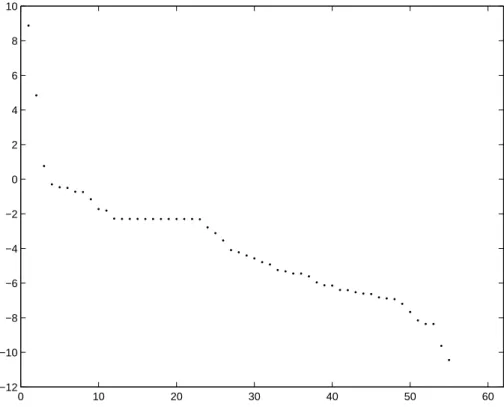
5

eigenvalues ofA. Figure1shows a typical eigenvalues distribution. Such a distribution justifies the need for a numerical solver dedicated to stiff equations.

In practice, we use the second order Rosenbrock method (seeVerwer et al.,1999):

c_n₊₁= c_n+ ∆tb₁k1+ ∆tb2k2 (2) where 10    k1= χ(tn,cn)+ ∆tγAk1 k2= χ(tn+ α12∆t, cn+ α21∆tk1) +∆tγ21Ak1+ ∆tγAk2 (3)

and α₁₂, α₂₁, γ₂₁and γ are prescribed coefficients and ∆t is the time step.

However this scheme is well suited in case of autonomous equations. Because of photochemistry and its dependence upon time (solar radiations), the equation to be solved is non-autonomous. As a consequence, the positivity of the solution may not be

15

preserved and negative concentrations are set to zero in order to avoid instabilities. A solution to retain positivity could also be to reduce the time step. Another solution is the stabilized Rosenbrock method (seeDjouad et al.,2002) where Eq. (3) is replaced with:    (I − γ∆tA) · k1= χ(tn,cn)+ γ∆t∂tχ (tn,cn) (I − γ∆tA) · k2= χ(tn+1,cn+ ∆tk1) −2k1− γ∆t∂tχ (tn,cn) (4) 20

(8)

ACPD

4, 1371–1392, 2004

3-D

Full Screen / Esc

which takes into account the time dependence of the production term χ . From our tests, the production-term non-autonomy and the time step (with which simulations are performed) are so that the non-autonomous scheme is not useful. However clipped masses are very small as compared to the whole pollutant masses. According to our tests, they can be neglected.

5

3.3. Cost reduction of the Rosenbrock integration

The main cost of the Rosenbrock method comes from the computations of k1and k2in

Eq. (3) which imply to solve a similar linear system twice. Its size is N×N where N is the number of chemical species. We use an LU factorization ofJ=I − γ∆tA. An important

feature ofJ is its sparsity: about 85% of matrix elements are zero. This is the reason

10

why the method proposed bySandu et al.(1996) can be very efficient. We permutate species so that the LU factorization ofJ remains sparse. This can be achieved by many

algorithms, one of which is the Markowitz algorithm. Moreover indices of non-zero entries are known a priori. Non-zero entries ofJ are deduced from species involved

in chemical reactions, and non-zero entries of its LU factorization can be determined

15

along with the factorization itself. Since indices of non-zero entries are known, it is possible to build tailored factorization and solver algorithms. They are usual algorithms from which useless computations (involving zero entries) were removed. Finally, we produce a code without indirect addressing (as in the Harwell-Boeing storage) also because indices of non-zero entries are known a priori.

20

This method dramatically reduces computational costs. For instance, the integration of the chemical mechanism RADM 2 (with 61 species) was speeded up by a factor of 3.6.

(9)

ACPD

4, 1371–1392, 2004

3-D

Full Screen / Esc

4. Validations

Two validations were conducted in order to assess model capabilities in non-academic cases. The first validation takes place over ˆIle de France, i.e. at regional scale. The second one tests the model at continental scale and over a long period (four months). 4.1. Validation at regional scale

5

The ESQUIF campaign investigated photo-oxidant pollution and led twelve intensive observation periods. IOP #2 occurred in August 1998 with low wind speeds (stagna-tion), a clear sky and high temperatures. This highly polluted episode has to be cor-rectly simulated by a model that aims at useful forecasts. The IOP #2 was simulated over ˆIle de France from 7 to 9 August 1998.

10

The 150 km×150 km domain is divided into 25 cells along x (6 km), 25 cells along y (6 km) and 9 cells along z (cell-centers altitudes being 15 m, 90 m, ... up to 2525 m). The top altitude of the last cell is 2800 m which seems reasonable according to the height of the boundary layer. We have taken a fixed time step of 600 s.

The main chemical mechanism was RADM 2 (see Stockwell et al., 1990), with 61

15

species and 157 reactions. The same simulation was performed with the chemical mechanism MOCA, with 66 chemical species and 126 reactions. However only results from RADM 2 will be analyzed here since both chemical mechanisms gave very similar results. Initial and boundary conditions come from output concentrations of the 3-D CTM Chimere (Vautard et al., 2001). Dry deposition velocities are assumed to be

20

constant.

A simulation takes less than 2 min per day on an Intel Pentium IV, 2 Ghz, and with the Intel Fortran Compiler.

Results for ozone at four stations are shown on Fig. 2. They were linearly inter-polated from output concentrations of Polair. Figure 2a – station Paris 18 – shows a

25

reasonable agreement with measurements inside Paris. Peaks are well forecast and grow from one day to the other due to stagnant conditions. Figure2b – station

(10)

Ram-ACPD

4, 1371–1392, 2004

3-D

Full Screen / Esc

bouillet – demonstrates a good behavior for the two last days. However the first day is not correctly simulated. Rambouillet was located in Paris plume (south west) and was highly dependent on simulated concentrations inside Paris. However initial conditions at Rambouillet and along the plume come from a continental model, which means that the first day is constrained by erroneous concentrations that cannot resolve the plume.

5

Figure 2c – Aubervilliers – shows overestimated concentrations at a station close to Paris 18 but outside Paris (north east) and its plume. The reason for this overestima-tion is not identified. This may come from lack of biogenic emissions or from bound-ary conditions. Biogenic emissions were not included because there were simply not available in Polair (at the time – it is not the case anymore). Moreover, a chemical

10

mechanism like RADM 2 is not perfectly suited to deal with biogenic emissions. One may use RACM instead. Figure2d – Montg ´e en Go ¨ele – is a rural station which is not in the plume. The first day is not well simulated because of initial conditions. The two other days show again an overestimation, as for station Aubervilliers.

Figure 2summarizes what is observed at other stations. The first day suffers from

15

initial conditions. As for the other days, results at stations within Paris and its plume are reasonably close to measurements. Those results are driven by rather fine data like anthropogenic emissions. Outside Paris and its plume, results are not as good as expected and are overestimated. At stations above the first level (30 m), improvements are needed as well.

20

To assess the whole results, the root mean square between computed concentra-tions and measurements is considered for all staconcentra-tions and over the three days. The mean over all stations of the root mean square is 39 µg·m−3, for an episode with high ozone concentrations. The correlation is 86%, which indicates a good time evolution for Polair outputs.

25

Improvements should be obtained with better input fields. Meteorological data could be processed in a better way, deposition velocities should be computed thanks to

We-sely (1989) or Baer et al. (1992) which are now available in the code, biogenic emis-sions should improve results specially outside the plume.

(11)

ACPD

4, 1371–1392, 2004

3-D

Full Screen / Esc

4.2. Validation at continental scale

At continental scale, a simulation over more than four months (from May to August 2001) demonstrates the validity of the model. This period gathers interesting episodes and is thus a complete validation in summer conditions.

The domain is (40.25◦N, 10.25◦W)×(57.25◦N, 22.75◦E), with 0.5◦×0.5◦ cells,

5

namely 33 cells along latitude and 65 cells along longitude. There are only 5 cells along z whose centers are 25 m, 325 m, 900 m, 1600 m and 2500 m. The top height of the last cell is 3000 m. The time step is 600 s, even if a larger time step should be acceptable. The chemical mechanism is RACM.

The purpose of this section is not to get into details about this simulation.

How-10

ever let us review quickly input data. Meteorological data comes from the ECMWF, anthropogenic emissions are provided by the EMEP database, biogenic emissions are estimated as inSimpson et al. (1999), initial and boundary conditions are extracted from Mozart-2 (Horowitz et al.,2003) output data. Vertical diffusion is estimated by the Louis parameterization (Louis,1979). Deposition velocities are computed according to

15

Wesely(1989).

Measurements from 242 stations (assumed to be background stations) are available. The mean of root mean squares at those stations is 29.7 µg·m−3 (computed with all measurements, i.e. hourly measurements) and is 24.7 µg·m−3 for concentrations at 15:00 UTC. The correlation is 60% (all measurements) and is 66% for concentrations

20

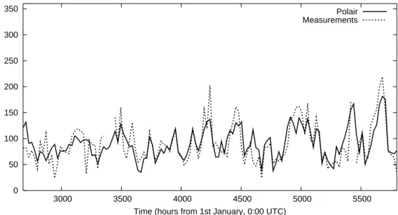
at 15:00 UTC. Those preliminary results show a good agreement with measurements. Figures3 and4show ozone peaks over the four months at two stations where root mean squares (25.2 µg·m−3 and 24.5 µg·m−3respectively) are close to the mean of all root mean squares (24.7µg·m−3). Figure5 shows a scatter plot of measurements of ozone concentrations at 15:00 UTC versus concentrations computed by Polair.

25

Those preliminary results seem good enough to let one be confident in the model. Compared to other models in very similar conditions (e.g. through the Pioneer forecasts –http://euler.lmd.polytechnique.fr/pioneer/), the results are satisfactory.

(12)

ACPD

4, 1371–1392, 2004

3-D

Full Screen / Esc

They will enable one way nesting and therefore should improve simulations at re-gional scale (by providing boundary conditions from the same model and with the same chemical mechanism). Moreover they allow to perform meaningful data assimilation.

5. Inverse-modeling strategy

Polair was designed to be well suited for data assimilation, notably thanks to the

avail-5

ability of a tangent linear mode and an adjoint mode. In this section, we provide details about this feature and we present an application.

5.1. Tangent linear and adjoint modes

Let us consider Polair as a function that takes input parameters (meteorological fields, emissions, etc.) and returns concentration fields. If one can get derivatives of

Po-10

lair output fields with respect to input parameters, one can get sensitivities of output concentrations to input parameters and one can build inverse modeling experiments or data assimilation experiments involving variational methods. Derivatives of Polair would therefore be of high interest.

Now, Polair can be automatically differentiated, i.e. one can get a code that returns

15

derivatives of output concentrations (as computed by Polair) with respect to input pa-rameters. Written in Fortran 77, it is differentiated by O∂yss´ee (Faure et al., 1998), which provides the tangent linear code and the adjoint code of Polair. From those codes, derivatives (previously described) are available.

No modification in Polair is required. However, to enforce computational efficiency,

20

we only replace the differentiated code of the LU factorization and the LU solver. To get such a simple procedure, the code was carefully built. For example, input/output oper-ations (which are not differentiable) and numerical integration have been separated.

Moreover the use of the differentiated code is straightforward since input/output sub-routines remain relevant. Loosely speaking, the numerical integration over one time

(13)

ACPD

4, 1371–1392, 2004

3-D

Full Screen / Esc

step is replaced by its differentiated code and the whole structure around it doesn’t change. In practice, it means that we can easily get the differentiated code with respect to virtually any parameter and for any simulation. Notice that absolutely all processes are differentiated: chemistry, diffusion, advection, deposition, etc.

Actually the main step is to validate the differentiated code by comparison with finite

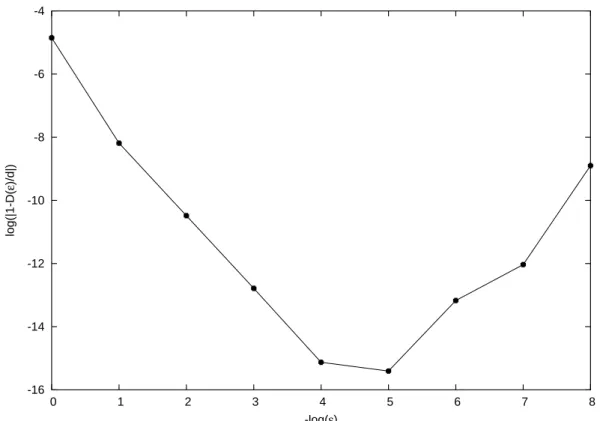
5

differences. This is performed with simulations involving all processes but at low costs (e.g. a few cells are enough). A derivative D(ε) is computed by finite differences (i.e. by computing the difference between a reference simulation and a slightly perturbed simulation) and compared to the differentiated-code output d. As the perturbation ε becomes smaller, finite differences should return a result closer to the

differentiated-10

code result d . If the perturbation is too small, round-off errors destroy finite differences accuracy. A relevant test is therefore to compute the ratio between the finite-difference result and the differentiated-code result as function of the perturbation. Figure 6 dis-plays results of such a (successful) test.

The computational cost of the differentiated code is more or less a function of the

15

forward code cost. The tangent linear code costs twice as much as the forward code, and the adjoint code cost is between 4.5 and 7 times the forward code cost.

5.2. Application

An application of such a code may be sensitivity analysis. One may consider an output variable (e.g. a 3-D field of ozone concentrations, or a given cost function) and may

20

need the derivative of this variable with respect to a set of parameters. This could be useful in order to choose relevant parameters for data assimilation: the more a variable is sensitive to a given parameter, the more relevant the parameter is. Such sensitivity analyses only provide local sensitivities. Nevertheless if several studies are performed in different situations, a very detailed analysis can be led and can provide results that

25

encompass enough cases to describe global sensitivities.

We performed, at both regional and continental scales, sensitivity analysis of ozone, nitrogen oxide and nitrogen dioxide concentrations to emissions of many chemical

(14)

ACPD

4, 1371–1392, 2004

3-D

Full Screen / Esc

species. Analyses of results are beyond the scope of this paper.

As soon as relevant parameters are chosen (with or without the use of the di fferen-tiated code), inverse modeling and data assimilation (4-D variational method) can be led thanks to the adjoint code. Currently, inverse modeling of emissions by use of the adjoint code is under progress.

5

6. Conclusions

We have summarized the main features of the chemistry-transport model Polair. Two simulations at regional and continental scales have shown a reasonable agreement with measurements. Thanks to those validations and the availability of differentiated versions of Polair, sensitivity studies and data assimilation can be performed. The main

10

future works will be devoted to aerosol modeling and air-quality ensemble forecast.

Acknowledgements. We thank I. Coll (LISA, Universit ´e Paris 12) for her help (simulation

at regional scale), R. Vautard (LMD, ´Ecole Polytechnique) and C. Honor ´e (Ineris) for their

help (simulation at European scale), Airparif (monitoring air quality in the Paris region) for its emission data base over ˆIle de France, and all monitoring networks that have made

15

comparisons with measurements possible at European scale. Edited by: J. Brandt

References

Aumont, B.: Mod élisation de la chimie de la basse troposph ère continentale: d éveloppement

20

et test d’un mod `ele chimique condens ´e, PhD thesis, Univ. Paris VII, 1994. 1374

Baer, M. and Nester, K.: Parametrization of trace gas dry deposition velocities for a regional

mesoscale diffusion model, Ann. Geophys., 10, 912–923, 1992. 1374,1379

Byun, D. W., Young, J., Gipson, G., Godowitch, J., Binkowsk, F., Roselle, S., Benjey, B., Pleim, J., Ching, J. K. S., Novak, J., Coats, C., Odman, T., Hanna, A., Alapaty, K., Mathur, R.,

(15)

ACPD

4, 1371–1392, 2004

3-D

Full Screen / Esc

McHenry, J., Shankar, U., Fine, S., Xiu, A., and Jang, C.: Description of the Models-3 Com-munity Multiscale Air Quality (CMAQ) model, Proceedings of the American Meteorological

Society 78th Annual Meeting, 264–268, 1998. 1372

Djouad, R., Sportisse, B., and Audiffren, N.: Numerical simulation of aqueous-phase

atmo-spheric models: use of a non-autonomous Rosenbrock method, Atmoatmo-spheric Environment,

5

36, 873–879, 2002. 1375,1376

Faure, C. and Papegay, Y.: O∂yss ´ee User’s Guide, version 1.7, Rapport technique 0224, INRIA,

France, 1998. 1381

Gery, M. W., Whitten, G. Z., Killus, J. P., and Dodge, M. C.: A photochemical kinetics mecha-nism for urban and regional scale computer modeling, J. Geophys. Res., 94, 12 925–12 956,

10

1989. 1374

Hass, H., Jakobs, H. J., and Memmesheimer, M.: Analysis of a regional model (EURAD) near surface gas concentration predictions using observations from networks, Meteorol. Atmos.

Phys., 57, 173–201, 1995. 1372

Horowitz, L. W., Walters, S., Mauzerall, D. L., Emmons, L. K., Rasch, P. J., Granier, C., Tie,

15

X., Lamarque, J.-F., Schultz, M. G., Tyndall, G. S., Orlando, J. J., and Brasseur, G. P.: A global simulation of tropospheric ozone and related tracers: Description and evaluation of

MOZART, version 2, J. Geophys. Res., 108, D24, 2003. 1380

Issartel, J.-P. and Baverel, J.: Inverse transport for the verification of the Comprehensive Test

Ban Treaty, Atmos. Chem. Phys., 3, 475–486, 2003. 1372

20

Louis, J. F.: A parametric model of vertical eddy fluxes in the atmosphere, Boundary Layer

Met., 17, 187–202, 1979. 1374,1380

Mallet, V.: AtmoData library: data processing and parameterizations in atmospheric sciences,

Tech. Rep. CEREA, 2004. 1375

Middleton, P., Stockwell, W. R., and Carter, W. P. L.: Aggregation and analysis of volatile organic

25

compound emissions for regional modeling, Atmospheric Environment, 24A, 1107–1133,

1990. 1374

Petersen, G., Iverfeldt, A., and Munthe, J.: Atmospheric mercury species over central and northern Europe, Model calculations and comparison with observations from the nordic air and precipitation network for 1987 and 1988, Atmospheric Environment, 29, 47–67, 1995.

30

1374

Roustan, Y. and Musson-Genon, L.: Rapport d’avancement – Plan de th `ese , Tech. Rep.

(16)

ACPD

4, 1371–1392, 2004

3-D

Full Screen / Esc

Sandu, A., Potra, F. A., Damian, V., and Carmichael, G. R.: Efficient implementation of fully implicit methods for atmospheric chemistry, Journal of Computational Physics, 129, 101–

110, 1996. 1377

Sartelet, K. N., Boutahar, J., Qu ´elo, D., Coll, I., Plion, P., and Sportisse, B.: Development and validation of a 3D Chemistry-Transport Model, POLAIR3D, by comparison with data

5

from ESQUIF campaign, Proceedings of the 6th Gloream workshop: Global and regional

atmospheric modelling, 2002. 1372

Schell, B.: Die Behandlung sekund ¨arer organischer Aerosole in einem komplexen

Chemie-Transport-Modell, PhD thesis, Univ. Cologne, 2000. 1374

Simpson, D., Winiwarter, W., B ¨orjesson, G., Cinderby, S., Ferreiro, A., Guenther, A., Hewitt,

10

C. N., Janson, R., Khalil, M. A. K., Owen, S., Pierce, T. E., Puxbaum, H., Shearer, M., Skiba,

U., Steinbrecher, R., Tarras ´on, L., and ¨Oquist, M. G.: Inventorying emissions from nature in

Europe, J. Geophys. Res., 104, 8113–8152, 1999. 1380

Spee, E.: Numerical methods in global transport models, PhD thesis, Univ. Amsterdam, 1998.

1375

15

Sportisse, B.: An analysis of operator splitting techniques in the stiff case, Journal of

Compu-tational Physics, 161, 140–168, 2000. 1375

Sportisse, B. and du Bois, L.: Numerical and theoretical investigation of of a simplified model for the parameterization of below-cloud scavenging by falling raindrops, Atmospheric

Envi-ronment, 36, 5719–5727, 2002. 1374

20

Stockwell, W. R., Kirchner, F., Kuhn, M., and Seefeld, S.: A new mechanism for regional

atmo-spheric chemistry modeling, J. Geophys. Res., 102, 25 847–25 879, 1997. 1374

Stockwell, W. R., Middleton, P., Chang, J. S., and Tang, X.: The second regional acid deposition model chemical mechanism for regional air quality modeling, J. Geophys. Res., 95, 16 343–

16 367, 1990. 1374,1378

25

Vautard, R., Beekmann, M., Roux, J., and Gombert, D.: Validation of a hybrid forecasting system for the ozone concentrations over the Paris area, Atmospheric Environment, 35,

2449–2461, 2001. 1372,1378

Verwer, J. G., Spee, E. J., Blom, J. G., and Hundsdorfer, W.: A Second-Order Rosenbrock Method Applied to Photochemical Dispersion Problems, SIAM J. Sci. Comput., 20, 1456–

30

1480, 1999. 1376

Walmsley, J. L. and Wesely, M. L.: Modification of coded parametrizations of surface resis-tances to gaseous dry deposition, Atmospheric Environment, 30, 1181–1188, 1996.

(17)

ACPD

4, 1371–1392, 2004

3-D

Full Screen / Esc

Wesely, M. L.: Parameterization of surface resistances to gaseous dry deposition in regional-scale numerical models, Atmospheric Environment, 23, 1293–1304, 1989.

375

(18)

ACPD

4, 1371–1392, 2004

3-D

Full Screen / Esc

Fig. 1. Absolute values of eigenvalues of a Jacobian matrix coming from chemical mechanism

RADM 2. The y-axis is a log-scale. Eigenvalues are strongly spread, from 109 to 10−11 and

(19)

ACPD

4, 1371–1392, 2004

3-D

Full Screen / Esc

Print Version Interactive Discussion © EGU 2004 (a) 00 10 20 30 40 50 60 70 20 40 60 80 100 120 140 160 180 200 Time (h) Concentration ( µ g ⋅ m −3 ) Measurements Polair 0 10 20 30 40 50 60 70 0 50 100 150 200 250 300 Time (h) Concentration ( µ g ⋅ m −3) Measurements Polair (c) (b) 00 10 20 30 40 50 60 70 20 40 60 80 100 120 140 160 180 Time (h) Concentration ( µ g ⋅ m −3) Measurements Polair 0 10 20 30 40 50 60 70 0 20 40 60 80 100 120 140 160 180 200 Time (h) Concentration ( µ g ⋅ m −3 ) Measurements Polair (d) Fig. 2. Ozone simulated (from 7 to 9 August 1998) concentrations at: (a) Paris 18, (b)

(20)

ACPD

4, 1371–1392, 2004

3-D

Full Screen / Esc

Time (hours from 1st January, 0:00 UTC)

Polair Measurements

Fig. 3. Ozone peaks (15:00 UTC) for each day of the simulation (from 27 April to 31 August

(21)

ACPD

4, 1371–1392, 2004

3-D

Full Screen / Esc

Time (hours from 1st January, 0:00 UTC)

Polair Measurements

Fig. 4. Ozone peaks (15:00 UTC) for each day of the simulation (from 27 April to 31 August

(22)

ACPD

4, 1371–1392, 2004

3-D

Full Screen / Esc

Fig. 5. Scatter plot of measurements (at all stations) of ozone concentrations at 15:00 UTC versus concentrations computed by Polair.

(23)

ACPD

4, 1371–1392, 2004

3-D

Full Screen / Esc

Fig. 6. Comparison between the derivative D(ε) as estimated by finite differences and the

derivative d computed by the automatically differentiated code. The ratio tends to 1 until round-off errors destroy finite-difference accuracy.