LATVIAN JOURNAL OF PHYSICS AND TECHNICAL SCIENCES 2017, N 6
DOI: 10.1515/lpts-2017-0041
APPLIED PHYSICS NUMERICAL APPROACH OF A WATER FLOW IN AN UNSATURATED POROUS MEDIUM BY COUPLING BETWEEN THE NAVIER–STOKES AND
DARCY–FORCHHEIMER EQUATIONS K. Hami1,2, I. Zeroual1
1Institute of Science and Technology,
University Center of Tindouf, Tindouf, 37000, ALGERIA 2Laboratory of Energetic in the Arid Areas ENERGARID,
Faculty of Technology, University Tahri Mohammed, Béchar, 08000, ALGERIA [email protected]
In the present research, simulations have been conducted to determine numerically the dynamic behaviour of the flow of underground water fed by a river. The basic equations governing the problem studied are those of Na-vier–Stokes equations of conservation of momentum (flows between pores), coupled by the Darcy–Forchheimer equations (flows within these pores). To understand the phenomena involved, we first study the impact of flow rate on the pressure and the filtration velocity in the underground medium, the second part is devoted to the calculation of the elevation effect of the river water on the flow behaviour in the saturated and unsaturated zone of the aquifer.
Keywords: Darcy–Forchheimer equations, groundwater flow, hydrody-namic modelling, porous medium
1. INTRODUCTION
The particularity of the reinforcements considered in the research is the pres-ence of several scales of porosity. On the one hand, the flow is modelled in the pores by the law of Darcy–Forchheimer, and on the other hand, it is modelled between the pores by the Navier–Stokes equations. The authors of the research, therefore, have a domain containing both a porous medium and a fluid zone.
This problem has already been studied for a long time, since Beavers and Joseph [1] study the flows of Navier–Stokes and speak already in their introduction about extensive analytical literature. They show the existence of the velocity of slip on the surface of the porous environment and propose a boundary condition. There-after, Saffman [2] justified this boundary condition mathematically and showed that the term velocity of Darcy could be neglected. It thus gave the condition known under the name of condition of Beavers–Joseph–Saffman. Certain digital studies concerning the coupling of the equations of Stokes and Darcy take into account this boundary condition, while others do not consider it.
Many authors have coupled the Navier–Stokes equations for the fluid area and Darcy’s equation for the porous zone. Correa and Loula [3] propose a coupling between a Navier–Stokes finite element formulation and a Darcy mixed formulation using Taylor-Hood elements.
J. M. Urquiza et al. [4] have presented a mixed finite element formulation of the Navier–Stokes with a formulation of the equation of Darcy taken in the form of a Poisson’s equation.
G. Pacquaut et al. [5] express the weak formulation of each equation by in-tegrating the condition of Beavers–Joseph–Saffman. Taking into account the boun-dary conditions being common to each formulation, they could inject the equation of Darcy directly in the formulation of Navier-Stokes, which allowed for the coupling. In principle, this makes the weak formulation of the equation of Brinkman.
G. N. Gatica et al. [6] use also a coupling of (Navier–Stokes)–Darcy equations to compare several types of elements to achieve a stable formulation. Once again, the resolved wording finally returns a weak formulation of the Brinkman equation. Masud [7] makes the same type of study by clearly solving the Brinkman equation, which he writes under his strong formulation, but calling it the Navier–Stokes–Darcy equation.
H. Tan and K. M. Pillai [8] also propose a finite element formulation of the Brinkman equations. However, they propose a modified Brinkman equation to take into account a stress jump at the fluid-porous interface.
The coupling between the equations of Darcy and Navier–Stokes was largely studied before by using the finite volume method (FVM) in the immersion of fields, because of the many applications utilising the heat transfer in the porous environ-ments and to the interface between the porous environment and the external fluid [9]– [10]. The technique of immersion of fields used was improved thereafter [11]–[14].
2. SIMULATION PROCEDURES 2.1. Mathematical Model
The equations which govern the problem treated (2) (3) and (5) are those of Navier–Stokes (flow between the pores) coupled by the Darcy–Forchheimer equa-tions (flows inside these pores) expressing respectively the conservation of mass and momentum.
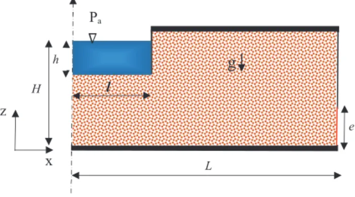
(H = 50 m, L = 100 m); (h = 5 m, l = 20 m); e = 10 m. Pa = 105 Pascal.
2.1.1. Equation: Porous Jump
(1)
where μ is the dynamic fluid viscosity, Δm is the thickness of the medium coefficient, v is the velocity normal to the porous face, α is the permeability of the medium and C2 is the pressure jump coefficient. α, Δm and C2 are parameters of boundary condi-tions specified by the user. In laminar flows through porous media, the pressure drop is typically proportional to velocity and the constant C2 can be considered to be zero, ignoring convective acceleration and diffusion.
2.1.2. Equation: Continuity
(2)
The equation is obtained by considering the mass flux into a representative elementary volume (R.E.V) to the increase of the fluid within the volume.
2.1.3. Equation: Navier-Stokes
Porous media are modelled through the addition of momentum source in terms of the governing equation of fluid flow. The sink term presented as equations (4) and (6) is assembled of two parts, of which Darcy law represents the left part and the right part considers the force of inertia.
and are the source term for the i-th (x, z) directions in the momentum equa-tions (4) and (6).
X-momentum:
(3)
Z-momentum:
(5)
(6)
where α is the permeability and C2 is the inertial resistance factor. 2.2. Boundary Conditions
• No slip conditions on the walls: (u = w =0); • Inlet flow:
(7)
• Outlet flow:
• Symmetry conditions:
• Impermeable surfaces:
The transport equations (2) (3) and (5) are resolved by the control volume method and solved by the SIMPLE algorithm [15]–[16], according to the first order-implicit numerical scheme. The equations of the algebraic system obtained have been solved by the Gauss–Seidel iterative method. It is estimated that the
conver-gence is reached when the relativedifferencesof all the calculated variables, at the different nodes of the mesh, become less than 10-5 between two successive iterations. 2.3. The Validity of Darcy Law
The balance between viscous and inertial forces are expressed by a non-di-mensional parameter called the Reynolds number:
(8)
where Re is Reynolds number, ρ is fluid density, v is fluid velocity, d is the diameter of the passageway through which the fluid moves, μ is dynamic fluid viscosity.
The authors of the present research have proven theoretically by solving the Navier–Stokes equations in the case Re << 1 (that is, when the inertial terms are neg-ligible). The authors see that the Navier–Stokes equations are called “Stokes equa-tions”; this relationship is called the Stokes law and it is useful, for example, for calculating a sedimentation rate of fine particles (it is necessary that Re << 1).
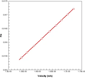
Fig. 2. The validity of Darcy’s law (Re vs. Velocity).
At high Reynolds numbers, the relationship between specific discharge and hydraulic gradient is no longer linear. Therefore, the transition zone of Reynolds numbers in the range of 1–10 is associated with the upper limit of Darcy’s law [17]. Such circumstances may occur in fracture flow and adjacent to wells that are pump-ing at high rates.
The lower limit of Darcy law (8) is associated with extremely slow ground-water movement. In such cases, other gradients, such as thermal, chemical and/or
electrical, may be stronger than the hydraulic gradient and may control the move-ment of flow.
The results shown in Fig. 2 demonstrate that regardless of the values taken by the pressure drop and the filtration rate the number of Re always remains less than 1. Thus, the criterion of Darcy is systematically validated in the studied cases.
2.4. Stationary Value for Pressure
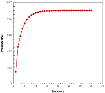
The evolution of the pressure of the groundwater flow in the vertical plane and in the middle of the aquifer studied (reference zone), represented in Fig. 3, comprises two successive phases, i.e., the transitional phase between the first iteration and the 10th iteration, which depends strongly on the initial state of the system, and the phase of established regime, or thence of the latter, independent of the initial state of the system (initial conditions).
Fig. 3. Stationary value for pressure (particular setup). 2.5. Test Meshes
For a gradually varied flow, it takes large longitudinal distances to observe significant changes in height; in areas where the flow rapidly varied, the meter is an acceptable longitudinal length scale. As the simulation is carried out over a distance of 100m of languor and 50m of depth, one can expect a realistic solution, placing a calculation node every meter. Then coarse meshes have been selected.
Thus, choosing a fine mesh, there is a clear solution of what the authors are willing to achieve. Conversely, for a coarse mesh, the authors have an estimate of the solution. The authors do not know how in practice an interpolation is done, but they believe that it is made without regard to the physical solution between two nodes.
The authors have calculated the residual values for each solution. Residues have been found in the same order of magnitude as the authors expected to have large residuals for coarse meshes.
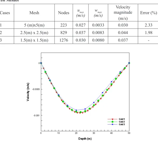
Table 1 Test Meshes
Cases Mesh Nodes umax
(m/s) (m/s)wmax Velocity magnitude (m/s) Error (%) 1 5 (m)x5(m) 223 0.027 0.0033 0.030 2.33 2 2.5(m) x 2.5(m) 829 0.037 0.0083 0.044 1.98 3 1.5(m) x 1.5(m) 1276 0.030 0.0080 0.037
-Fig. 4. Test meshes: (Velocity vs. Depth).
To sum up, if the number of nodes is increased, the number of errors is re-duced due to interpolation between the nodes, and the numerical solution is closer to reality. It has also been noted that the computation time increases with the fineness of the mesh, but this increase (Error < 2.33 %) is not significant for the meshes chosen in the present simulations.
3. INTERPRETATION OF RESULTS 3.1. Pressure Drop vs. Velocity
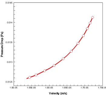
Fig. 5. Evolution of pressure vs. velocity.
It can be observed from Fig. 5 that pressure drop for clean water increases with increased inflow rate (feed rate). When the inlet feed rate increases, the tangen-tial velocity of flow in the aquifer increases. Thereby the centrifugal force on water molecules increases and gives high velocity. It has been found that the clean pressure drop varies 1.44 to the power of velocity as shown in equation 9.
(9)
where – clean pressure drop, Pa, and w – velocity, (m/s). 3.2. Streamlines and Velocity Field
It is observed in Fig. 6 that the flow of water into the aquifer moves in layers, which glide one over the other, without mixing, and the flow is laminar. The current streamlines traced in the fluid whose tangents at all points are parallel to the direction of flow and are generally curved but never intersect.
The flow is a flat flow, in a vertical direction from the river to the aquifer, on the one hand, and horizontal from the aquifer to the storage basin, on the other.
The velocity field demonstrated in Fig. 7 shows that the velocity is zero close to the impermeable walls due to the non-slip condition, the maximum values are observed at the level of water infiltration from the river to the aquifer and at the level of the aquifer towards the storage area.
Fig. 7. Streamlines and velocity field. 3.3. Pressure Drop Field
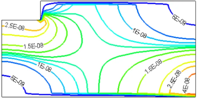
It is seen that the flows are organised according to the search for the most ad-vantageous outlets (Fig. 8) (evacuation of a maximum of flows with a minimum of losses of load). The observation of the load change in approaching the watercourse banks to identify what situation you are in. Thus, increasing loads towards the river show a river-slick flow.
Fig. 8. Pressure drop field. The piezometric lines are doubly influenced by:
• the general direction of flow of the water table (in accordance with the flow direction of the river in the general case).
• relations with the river, depending on whether it is supported by the groundwater or fed by the water table (a situation that can be reversed depending on the season and / or the intensity of the anthropogenic with-drawals in the groundwater).
4. CONCLUSIONS
This approach presents a coupling between the Darcy–Forchheimer equations and the mass and momentum conservation equations (Navier–Stokes) to describe these interactions (river / aquifer) on a local scale. The flow of water into the soil va-ries according to the multiplicity of paths taken by the drops of water. The interaction between rivers and aquifers describes the main phenomenon of infiltration (passage of water across the soil surface under the effect of gravity) that constitutes the path of groundwater. The flow of infiltrating water varies according to the influence of several physical and geological factors. These include percolation (flow of liquid in unsaturated soil due to gravity) and capillary rise (ascent of water above the under-ground water table by capillarity). The behaviour of these two phenomena is depen-dent on the properties of aquifers, especially hydraulic conductivity, as demonstrated by the Darcy experiment, which is the basis for the modelling of underground flows.
REFERENCES
1. Beavers, G.S., & Joseph, D.D. (1967). Boundary conditions at naturally permeable wall.
Journal of Fluid Mechanics, 30(1), 197–207.
2. Saffman, P.G. (1971). On the boundary condition at the surface of a porous medium.
Studies in Applied Mathematics, 50(2), 93–101.
3. Correa, M.R., & Loula, A.F.D. (2009). A unified mixed formulation naturally coupling Stokes and Darcy flows. Computer Methods in Applied Mechanics and Engineering,
198(33-36), 2710–2722.
4. Urquiza, J.M., N’Dri, D., Garon A., & Delfour, M.C. (2008). Coupling Stokes and Darcy equations. Applied Numerical Mathematics, 58(5), 525–538.
5. Pacquaut, G., Bruchon, J., Moulin N., & Drapier, S. (2011). Combining a level-set meth-od and a mixed stabilized P1/P1 formulation for coupling Stokes-Darcy flows.
Interna-tional Journal for Numerical Methods in Fluids, 66.
6. Gatica, G.N., Oyarzúa, R., & Sayas, F.-J. (2011). Convergence of a family of Galerkin discretizations for the Stokes-Darcy coupled problem. Numerical Methods for Partial
Differential Equations, 27(3), 721–748.
7. Masud, A. (2007). A stabilized mixed finite element method for Darcy-Stokes flow.
In-ternational Journal for Numerical Methods in Fluids, 54(6–8), 665–681.
8. Tan, H., & Pillai, K. M. (2009). Finite element implementation of jump and stress-continuity conditions at porous-medium, clear-fluid interface. Computers & Fluids,
38(6), 1118–1131.
9. Arquis, E., & Caltagirone, J.P. (1984). Sur les conditions hydrodynamiques au voisi-nage d’une interface milieu _uide-milieu poreux : application à la convection naturelle.
Comptes Rendus de l’Académie des Science de Paris, Série II, 299, 1–4.
10. Arquis, E., Caltagirone, J.P., & Le Breton, P. (1991). Détermination des propriétés de dispersion d’un milieu périodique à partir de l’analyse locale des transferts thermiques.
Comptes Rendus de l’Académie des Science de Paris, Série II, 313, 1087–1092.
11. Vincent, S., Caltagirone, J.-P., Lubin, P., & Randrianarivelo, T.-N. (2004). An adaptative augmented lagrangian method for three-dimensional multimaterial flows. Computers &
12. Randrianarivelo, T.N., Pianet, G., Vincent S., & Caltagirone, J.-P. (2005). Numerical modelling of solid particle motion using a new penalty method. International Journal for
Numerical Methods in Fluids, 47, 1245–1251.
13. Sarthou, A., Vincent, S., Caltagirone, J.-P., & Angot, P. (2008). Eulerian lagrangian grid coupling and penalty methods for the simulation of multiphase flows interacting with complex objects. International Journal for Numerical Methods in Fluids, 56, 1093–1099. 14. Puaux, G. (2011). Numerical simulation of flows at microscopic and mesoscopic scales
in RTM process. PhD thesis. École nationale supérieure des mines de Paris.
15. Patankar, S.V. (1980). Numerical Heat Transfer and Fluid Flow. Hémisphère Inc.: McGraw-Hill, Washington, États-Unis.
16. Versteeg, H.K, & Malalasekera, W. (1995). Introduction to Computational Fluid Dynam-ics: The Finite Volume Method. Wiley, New York, États-Unis.
17. Bear, J. (1972). Dynamics of fluids in porous media. Elsevier.
SKAITLISKĀ PIEEJA ŪDENS PLŪSMAS RAKSTUROŠANAI NEPIESĀTINĀTAJĀ PORAINĀ VIDĒ, APVIENOJOT NAVJĒ-STOKSA
UN DARSĪ-FORHEIMERA VIENĀDOJUMUS K. Hami, I. Zeroual
K o p s a v i l k u m s
Šajā pētījumā tika veiktas simulācijas, lai skaitliski noteiktu upes barotās pazemes ūdens plūsmas dinamiskos raksturlielumus. Pamata vienādojumi, kas regulē pētāmo problēmu, ir kustības daudzuma saglabāšanās jeb Navjē-Stoksa vienādojumi (plūsma starp porām), kurus apvieno ar Darsī-Forheimera vienādojumiem (plūsma šajās porās). Lai izprastu iesaistītās parādības, autori vispirms pēta plūsmas ātruma ietekmi uz spiedienu un filtrēšanas ātrumu pazemes vidē, pēc tam aprēķina upes ūdens līmeņa paaugstināšanās ietekmi uz plūsmas uzvedību ūdens nesējslāņa piesātinātajā un nepiesātinātajā daļā.