Real-time 2D manipulation of plausible 3D appearance using shading and geometry buffers

(1)

HAL Id: tel-01440828

https://hal.inria.fr/tel-01440828

Submitted on 19 Jan 2017

HAL is a multi-disciplinary open access

archive for the deposit and dissemination of

sci-entific research documents, whether they are

pub-lished or not. The documents may come from

teaching and research institutions in France or

abroad, or from public or private research centers.

L’archive ouverte pluridisciplinaire HAL, est

destinée au dépôt et à la diffusion de documents

scientifiques de niveau recherche, publiés ou non,

émanant des établissements d’enseignement et de

recherche français ou étrangers, des laboratoires

publics ou privés.

Real-time 2D manipulation of plausible 3D appearance

using shading and geometry buffers

Carlos J. Zubiaga

To cite this version:

Carlos J. Zubiaga. Real-time 2D manipulation of plausible 3D appearance using shading and geometry

buffers. Graphics [cs.GR]. Université de Bordeaux, 2016. English. �tel-01440828�

(2)

THESIS

PRESENTED AT

UNIVERSIT´

E DE BORDEAUX

´

ECOLE DOCTORALE DE MATHMATIQUES ET

D’INFORMATIQUE

par

Carlos Jorge Zubiaga Pe˜

na

POUR OBTENIR LE GRADE DE

DOCTEUR

SP´

ECIALIT´

E : INFORMATIQUE

Real-time 2D manipulation of plausible 3D appearance

using shading and geometry buffers

Date de soutenance : 7 November 2016

Devant la commission d’examen compose de :

Diego Gutierrez . . . Professeur, Universidad de Zaragoza . . . Rapporteur Daniel Sýkora _{. . . .} _{Professeur associé, Czech Technical University in Prague} _Rapporteur Pascal Guitton . . . Professeur, Univeristé Bordeaux . . . Président David Vanderhaeghe Maˆıtre de Conferences, Univeristé de Toulouse . . . Examinateur Xavier Granier . . . Professeur, Institut d’Optique . . . Examinateur Pascal Barla . . . Chargé de recherche, Inria . . . Directeur

(3)

(4)

of real-world scenes. In contrast, Computer Graphics artists define objects on a virtual scene (3D meshes, materials and light sources), and use complex algorithms (rendering) to reproduce their appearance. On the one hand, painting techniques permit to freely define appearance. On the other hand, rendering techniques permit to modify separately and dynamically the different elements that compose the scene.

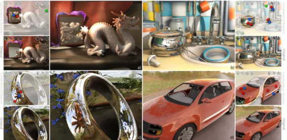
In this thesis we present a middle-ground approach to manipulate appearance. We offer 3D-like manipulation abilities while working on the 2D space. We first study the impact on shading of materials as band-pass filters of lighting. We present a small set of local statistical relationships between material/lighting and shading. These relationships are used to mimic modifications on material or lighting from an artist-created image of a sphere. Techniques known as LitSpheres/MatCaps use these kinds of images to transfer their appearance to arbitrary-shaped objects. Our technique proves the possibility to mimic 3D-like modifica-tions of light and material from an input artwork in 2D. We present a different technique to modify the third element involved on the visual appearance of an object: its geometry. In this case we use as input rendered images alongside with 3D information of the scene output in so-called auxiliary buffers. We are able to recover geometry-independent shading for each object surface, assuming no spatial variations for each recovered surface. The recovered shading can be used to modify arbitrarily the local shape of the object interactively without the need to re-render the scene.

Keywords Appearance, shading, pre-filtered environment map, MatCap, Compositing Résumé Les artistes traditionnels peignent directement sur une toile et créent des ap-parences plausibles de scènes qui ressemblent au monde réel. A l’opposé, les artistes en infor-matique graphique définissent des objets dans une scène virtuelle (maillages 3D, matériaux et sources de lumière), et utilisent des algorithmes complexes (rendu) pour reproduire leur ap-parence. D’un côté, les techniques de peinture permettent de librement définir l’apparence. D’un autre côté, les techniques de rendu permettent de modifier séparément et dynamique-ment les différents élédynamique-ments qui définissent l’apparence.

Dans cette thèse, nous présentons une approche intermédiaire pour manipuler l’apparence, qui permettent certaines manipulations en 3D en travaillant dans l’espace 2D. Mous étudions d’abord l’impact sur l’ombrage des matériaux, tenant en compte des matériaux comme des filtres passe-bande d’éclairage. Nous présentons ensuite un petit ensemble de relations statis-tiques locales entre les matériaux / l’éclairage et l’ombrage. Ces relations sont utilisées pour imiter les modifications sur le matériaux ou l’éclairage d’une image d’une sphère créée par un artiste. Les techniques connues sons le nom de LitSpheres / MatCaps utilisent ce genre d’images pour transférer leur apparence à des objets de forme quelconque. Notre technique prouve la possibilité d’imiter les modifications 3D de la lumière et de matériaux à partir d’une image en 2D. Nous présentons une technique différente pour modifier le troisième élément impliqué dans l’aspect visuel d’un objet, sa géométrie. Dans ce cas, on utilise des rendus comme images d’entrée avec des images auxiliaires qui contiennent des informations 3D de la scène. Nous récupérons un ombrage indépendant de la géométrie pour chaque surface, ce qui nous demande de supposer qu’il n’y a pas de variations spatiales d’éclairage pour chaque surface. L’ombrage récupéré peut être utilisé pour modifier arbitrairement la forme locale de l’objet de manière interactive sans la nécessité de rendre à nouveau la scène. Mots-clés Apparence, ombrage, cartes d’environnement pré-flitrées, MatCap, Composit-ing

(5)

(6)

Chapter 1 Introduction

One of the main goals of image creation in Computer Graphics is to obtain a picture which conveys a specific appearance. We first introduce the general two approaches of image creation in the Section1.1, either by directly painting the image in 2D or by rendering a 3D scene. We also present middle-ground approaches which work on 2D with images containing 3D information. It is important to note that our work will take place using this middle-ground approach. We define our goal in Section1.2 as ‘granting 3D-like control over image appearance in 2D space’. Our goal emerges from the limitations of existing techniques to manipulate 3D appearance in existing images in 2D. Painted images lack any kind of 3D information, while only partial geometric information can be output by rendering. In any case, the available information is not enough to fully control 3D appearance. Finally in Section1.3we present the contributions brought by the thesis.

1.1 Context

Image creation can be done using different techniques. They can be gathered into two main groups, depending if they work in the 2D image plane or in a 3D scene. On the one hand, traditional painting or the modern digital painting softwares work directly in 2D by assigning colors to a plane. On the other hand, artists create 3D scenes by defining and placing objects and light sources. Then the 3D scene is captured into an image by a rendering engine which simulates the process of taking a picture. There also exist techniques in between that use 3D information into 2D images to create or modify the colors of the image.

1.1.1 Painting

Traditional artists create images of observed or imagined real-world scenes by painting. These techniques are based on the deposition of colored paint onto a solid surface. Artists may use different kinds of pigments or paints, as well as different tools to apply them, from brushes to sprays or even body parts. Our perception of the depicted scene depends on intensity and color variations across the planar surface of the canvas. Generated images may be abstract or symbolic, but we are interested in the ones that can be considered as natural or realistic. Artists are capable to depict plausible appearances of the different elements that compose a scene. The complexity of reality is well captured by the design of object’s shape and color. Artists achieve good impressions of a variety of materials under different lighting environment. This can be seen in Figure 1.1, where different object are shown ranging from organic nature to hand-crafted.

(9)

1.1. Context

Bodegonby Francisco Zurbaran Still-lifeby Pieter Caesz Attributes of Musicby Anne Vallayer-Coster

Figure 1.1: Still-life is a work of art depicting inanimate subjects. Artists are able to achieve a convincing appearance from which we can infer the material of the different objects.

Nowadays painting techniques have been integrated in computer system environments. Classical physical tools, like brushes or pigments, have been translated to digital ones (Fig-ure1.2). Moreover, digital systems provide a large set of useful techniques like the use of different layers, selections, simple shapes, etc. They also provide a set of image based opera-tors that allow artists to manipulate color in a more complex way, like texturing, embossing or blurring. Despite the differences, both classical painting and modern digital systems share the idea of working directly in image space.

(a) ArtrageTM _{(b) Photoshop}TM

Figure 1.2: Computer systems offer a complete set of tools to create images directly in image space. They provide virtual versions of traditional painting tools, such as different kinds of brushes or pigments, as can be seen in the interface of ArtRageTM₍_a_{). On the right (}_b_{) we}

can see the interface of one of the most well-known image editing softwares, PhotoshopTM_.

They also provide other tools that couldn’t exist in traditional painting, like working on layers, different kind of selections or image modifications like scaling or rotations.

Artists are able to depict appearances that look plausible, in a sense that they look real even if they would not be physically correct. Despite our perception of the painted objects as if they were or could be real, artist do not control physical processes. They just manipulate colors either by painting them or performing image based operations. They use variations of colors to represent objects made of different materials and how they would behave under a different illumination. The use of achromatic variations is called shading; it is used to convey volume or light source variations (Figure 1.3), as well as material effects. Shading may also correspond to variations of colors, so we can refer to shading in a colored or in a grey scale image.

(10)

Figure 1.3: Shading refers to depicting depth perception in 3D models or illustrations by varying levels of darkness. It makes possible to perceive volume and infer lighting direction. Image are property of Kristy Kate http://kristykate.com/.

In real life, perceived color variations of an object are the result of the interaction between lighting and object material properties and shape. Despite the difficult understanding of these interactions, artists are able to give good impressions of materials and how they would look like under certain illumination conditions. However, once a digital painting is created it cannot be modified afterwards: shape, material, or lighting cannot be manipulated.

1.1.2 Rendering

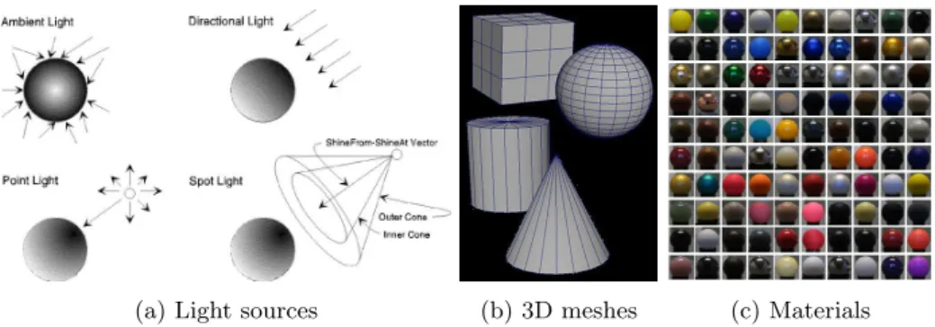
Contrary to 2D techniques, computer graphics provide an environment where artists define a scene based on physical 3D elements and their properties. Artists manipulate objects and light sources, they control object’s shape (Fig.1.4b) and material (Fig.1.4c) and the type of light sources (Fig. 1.4a), as well as their positions. When an artist is satisfied with the scene definition, he selects a point of view to take a snapshot of the scene and gets an image as a result.

(a) Light sources (b) 3D meshes (c) Materials

Figure 1.4: A 3D scene are composed of lights and objects. where lights may vary in type (a) from ambient, to point, direction, area, etc. Objects are defined by their geometry defined by (b) 3D meshes and (c) materials.

The creation of 2D images from a 3D scene is called rendering. Rendering engines are software frameworks that use light transport processes to shade a scene. The theory of light transport defines how light is emitted from the light sources, how it interacts with the different objects of the scene and finally how it is captured in a 2d plane. In practice, light rays are traced from the point of view, per pixel in the image. When the rays reach an object surface, rays are either reflected, transmitted or absorbed, see Figure1.5a. Rays continue their path until they reach a light source or they disappear by absorption, loss of energy or a limited number of reflections/refractions. At the same time, rays can also be traced from the light sources. Rendering engines usually mix both techniques by tracing rays from both directions, as shown in Figure1.6.

(11)

1.1. Context

(a) General material (b) Opaque material

Figure 1.5: In the general case, when a light ray reaches a object surface, it can be reflected, refracted or absorbed. When we focus on opaque objects the reflection can vary from shining (mirror) to matte (diffuse) by varying glossiness.

Figure 1.6: Rays may be both traced from the eye or image plane as well as from the light sources. When a ray reaches an object surface it is reflected, transmitted or absorbed.

Object geometry is defined by one or more 3D meshes composed of vertices, which form facets that describe the object surface. Vertices contain information about their 3D position, as well as other properties like their surface normal and tangent. The normal and tangent together describe a reference frame of the geometry at a local scale, which is commonly used in computer graphics to define how materials interact with lighting. This reference frame is used to define the interaction at a macroscopic level. In contrast, real-world interaction of light and a material at a microscopic level may turn out to be extremely complex. When a ray reaches a surface it can be scattered in any possible direction, rather than performing a perfect reflection. The way rays are scattered depends on the surface reflectance for opaque objects or the transmittance in the case of transparent or translucent objects. Materials are usually defined by analytical models with a few parameters; the control of those parameters allows artists to achieve a wide range of object appearances.

Manipulation of all the 3D properties of light, geometry and material allows artists to create images close to real-world appearances. Nevertheless, artists usually tweak images by manipulating shading in 2D until they reach the desired appearance. Those modifications are usually done for artistic reasons that require the avoidance of physically-based restrictions of the rendering engines, which make difficult to obtain a specific result. Artists usually start from the rendering engine output, from which they work to get their imagined desired image.

(12)

1.1.3 Compositing

Shading can be separated into components depending on the effects of the material. Com-monly we can treat independently shading coming from the diffuse or the specular reflec-tions (see Figure1.5b), as well as from the transparent/translucent or the emission effects. Therefore, rendering engines can outputs images of the different components of shading in-dependently. In the post-processing stage, called compositing, those images are combined to obtain the final image, as shown in Figure1.7.

Transparent Reflection Specular

Subsurface Luminous Diffuse

Final shading

Figure 1.7: Rendering engine computes shading per component: diffuse, reflections, trans-parency, etc. They generate per each component. Those images are used in post-process step called compositing. Final image is created as a combination of the different components. This figure shows an example from the software ModoTM_.

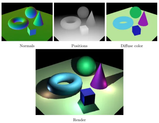
In parallel with shading images, rendering engines have the capacity to output auxiliary buffers containing 3D information. In general, one can output any kind of 3D information, by assigning them to the projected surface of objects in the image. Usually those buffers are used to test errors for debugging, but they can be used as well to perform shading modifications in post-process. They can be used to guide modifications of shading: for instance, positions or depth information are useful to add fog or create focusing effects like depth of fields. Auxiliary buffers may also be used to add shading locally. Having information about positions, normals and surface reflectance are enough to create new shading by adding local light sources. This is similar to a technique called Deferred Shading used in interactive rendering engines. It is based on a multi-pass pipeline, where the first pass produces the necessary auxiliary buffers and the other passes produce shading by adding the contribution of a discrete set of lights, as is shown in Figure1.8.

(13)

1.1. Context

Normals Positions Diffuse color

Render

Figure 1.8: Deferred shading computes in a first step a set of auxiliary buffers: positions, normals, diffuse color and surface reflectance. In a second pass those buffers are used to compute shading by adding the contribution of every single light source

Instead of computing shading at each pass we can pre-compute it, if we only consider distant illumination. Distant illumination means that there is no spatial variation on the incoming lighting, therefore it only depends on the surface normal orientation. Thanks to this approximation we only need surface normals to shade an object (usually they are used projected in screen space). Typically, pre-computed shading values per hemisphere direction are given by filtering the values of the environment lighting using the material reflectance properties. These techniques are referred by the name pre-filtered environment maps or PEM (see Chapter 2, Section 2.3). Different material appearances are obtained by using different material filters, as seen in Figure 1.9a. Pre-computed values are stored in spherical structures that can be easily accessed, shading is obtained by fetching using normal buffers. Instead of filtering an environment map, pre-computed shading values may also be created by painting or obtained from images (photographs or artwork). A well known technique, call the LitSphere, defines how to fill colors on a sphere from a picture and then use this sphere to shade an object, similarly to pre-filtered environment map techniques. The idea of LitSphere it’s been extensively used in sculpting software where it takes the name of MatCap (see Figure 1.9b), as shorthand of Material Capture. MatCaps depict plausible materials under an arbitrary environment lighting. In the thesis we decided to use MatCaps instead of LitSpheres to avoid misunderstanding with non photo-realistic shading, like cartoon shading. Despite the limitations of distant lighting (no visibility effects like shadows or inter-reflections), they create convincing shading appearances.

(14)

(a) Pre-filtered envirenmont maps

(b) MatCaps

Figure 1.9: Both pre-filtered environment maps (a) and MatCaps (b) can be used to shade arbitrary objects. Shading color per pixel is assigned by fetching the color that corresponds to the same normal in the spherical representation.

1.1.4 Summary

On the one hand, painting techniques permit direct manipulation of shading with no re-strictions, allowing artists to achieve the specific appearance they desire. In contrast, artists cannot manipulate dynamically the elements represented (object shape and material) and how they are lit. On the other hand, global illumination rendering engines are based on a complete control of the 3D scene and a final costly render. Despite the complete set of tools provided to manipulate a scene before rendering, artists commonly modify the rendering output in post-processing using image-based techniques similar to digital painting. Post-process modifications permit to avoid the physically based restrictions of the light transport algorithms.

As a middle-ground approach between the direct and static painting techniques and the dynamically controlled but physically-based restricted render engines, we find techniques which work in 2D and make use of 3D information in images or buffers. Those techniques may be used in post-process stage called compositing. Rendering engines can easily output image buffers with 3d properties like normal, positions or surface reflectance, which are usually called auxiliary buffers. Those buffers permit to generate or modify shading in ways different than digital painting, like the addition of local lighting or a few guided image operations (i.e. fog, re-texturing). Modifications of the original 3D properties (geometry, material or lighting) cannot be performed with a full modification on shading. A different way to employ auxiliary buffers is to use normal buffers alongside with pre-filtered environment maps or MatCaps/LitSpheres to shade objects. The geometry of the objects can be modified arbitrarily, but in contrast once pre-computed shading is defined, their depicted material and lighting cannot be modified.

(15)

1.2. Problem statement

1.2 Problem statement

Dynamic manipulation of appearance requires the control of three components: geometry, material and lighting. When we obtain an image independently of the way it has been created (painted or rendered) we lose the access to all components. Geometry is easily accessible, normal buffers may be generated by a rendering engine, but also may be obtained by scanners or estimated from images. Material are only accessible when we start from a 3D scene; the reflectance properties of the object can be projected to the image plane. Lightingin contrast is not accessible in any case. If we consider rendering engines, lighting is lost in the process of image creation. In the case of artwork, shading is created directly and information of lighting and materials is ‘baked-in’, therefore we do not have access to lighting or material separately.

Lighting structure is arbitrary complex and the incoming lighting per surface point varies in both the spatial and the angular domain, in other words, it varies per position and normal. The storage of the full lighting configuration is impractical, as we would need to store a complete environment lighting per pixel. Moreover, in the ideal case that we would have access to the whole lighting, the modification of the material, geometry or lighting will require a costly re-rendering process. In that case there will not be an advantage compared to rendering engine frameworks.

Our goal is to grant 3D-like control of image appearance in 2D space. We want to incorporate new tools to modify appearance in 2D using buffers containing 3D information. The objective is to be able to modify lighting, material and geometry in the image and obtain a plausible shading color. We develop our technique in 2 steps: first, we focus on the modification of light and material and then on the modification of geometry.

We base our work on the hypothesis that angular variations due to material and lighting can be mimicked by applying modifications directly on shading without having to decouple material and lighting explicitly. For that purpose we use structures similar to pre-filtered environment maps, where shading is stored independently of geometry.

In order to mimic material and lighting variations, we focus MatCaps. They are artist-created images of spheres, which their shading depicts an unknown plausible material under an unknown environment lighting. We want to add dynamic control over lighting, like rota-tion, and also to the material, like modifications of reflectance color, increasing or decreasing of material roughness or controlling silhouette effects.

In order to mimic geometry modifications, we focus on the compositing stage of the image creation process. Perturbations of normals (e.g. Bump mapping) is a common tool in computer graphics, but it is restricted to the rendering stage. We want to grant similar solutions of the compositing stage. In this stage several shading buffers are output by a global illumination rendering process and at the same time several auxiliary buffers are made available. Our goal in this scenario is to obtain a plausible shading for the modified normals without having to re-render the scene. The avoidance of re-rendering will permit to alter normals interactively.

As described in the previous section, material reflectance, and as a consequence shad-ing, can be considered as the addition of specular and diffuse components. Following this approach we may separate the manipulation of diffuse from specular reflections, which is sim-ilar to control differently low-frequency and high-frequency shading content. This approach can be considered in both cases, the MatCap and the compositing stage, see Figure1.10. Meanwhile rendering engines can output both components separately, MatCaps will require a pre-process step to separate them.

(16)

+

=

(a) MatCap

+

=

(b) Rendering

Figure 1.10: Shading is usually composed as different components. The main components are diffuse and specular reflections. We can see how (a) a MatCap and (b) a rendering are composed as the addition of a diffuse and a specular component.

1.3 Contributions

The work is presented in three main chapters that capture the three contributions of the thesis. Chapter3 present a local statistical analysis of the impact of lighting and material on shading. We introduce a statistical model to represent surface reflectance and we use it to derive statistical relationships between lighting/material and shading. At the end of the chapter we validate our study by analyzing measured materials using statistical measure-ments.

In Chapter4 we develop a technique which makes use of the statistical relationships to manipulate material and lighting in a simple scene: an artistic image of a sphere (MatCap). We show how to estimate a few statistical properties of the depicted material on the MatCap, by making assumptions on lighting. Then those properties are used to modify shading by mimicking modifications on lighting or material, see Figure1.11.

(a) Input MatCap (b) Rotated lighting (c) Color change (d) Rougher look

Figure 1.11: Starting from a stylized image of a sphere (a) our goal is to vary the (b) lighting orientation, (c) the material color and (d) the material roughness.

(17)

1.3. Contributions Chapter 5 introduces a technique to manipulate local geometry (normals) at the com-positing stage; we obtain plausible diffuse and specular shading results for the modified normals. To this end, we recover a single-view pre-filtered environment map per surface and per shading component. Then we show how to use these recovered pre-filetered environ-ment maps to obtain plausible shading when modifications on normals are performed, see Figure1.12.

Figure 1.12: Starting from shading and auxiliary buffers, our goal is to obtain a plausible shading color when modifying normals at compositing stage.

(18)

Chapter 2 Related Work

We are interested in the manipulation of shading in existing images. For that purpose we first describe the principles of rendering, in order to understand how virtual images are created as the interaction of geometry, material and lighting (Section2.1). Given an input image a direct solution to modify its appearance is to recover the depicted geometry, material and lighting. These set of techniques are called inverse rendering (Section2.2). Recovered components can be modified afterwards and a new rendering can be done. Inverse rendering is limited as it requires assumptions on lighting and materials which forbids its use in general cases. These techniques are restricted to physically-based rendering or photographs and they are not well defined to work with artworks. Moreover, a posterior rendering would limit the interactivity of the modification process. To avoid this tedious process, we found interesting to explore techniques that work with an intermediate representation of shading. Pre-filtered environment maps store the results of the interaction between material and lighting independently to geometry (Section2.3). These techniques have been proven useful to shade objects in interactive applications, assuming distant lighting. Unfortunately there is no technique which permits to modify lighting or material once PEM are created.

Our work belongs to the domain of appearance manipulation. These techniques are based on the manipulation of shading without the restrictions of physically-based rendering (Section2.4). However, the goal is to obtain images which appear plausible even if they are not physically correct. Therefore we also explore how the human visual system interprets shading (Section2.5). We are interested into our capability to infer the former geometry, lighting and material form an image.

2.1 Shading and reflectance

We perceive objects by the light they reflect toward our eyes. The way objects reflect light depends on the material they are composed of. In the case of opaque objects it is described by their surface reflectance properties; incident light is considered either absorbed or reflected. Surface reflectance properties define how reflected light is distributed. In contrast, for transparent or translucent objects the light penetrates, scatters inside the object and eventually exists from a different point of the object surface. In computer graphics opaque object materials are defined by the Bidirectional Reflectance Distribution Functions (BRDF or fr), introduced by Nicodemus [Nic65]. They are 4D functions of an incoming ωi

and an outgoing direction ωo(e.g., light and view directions). The BRDF characterizes how

much radiance is reflected in all lighting and viewing configurations, and may be considered as a black-box encapsulating light transport at a microscopic scale. Directions are classically parametrized by the spherical coordinates elevation θ and azimuth φ angles, according to the reference frame defined by the surface normal n and the tangent t as in Figure2.1a.

(19)

2.1. Shading and reflectance n t ωo ωi φ i φ_o θo θ i

(a) Classical parametrization

n t h θd θh ωo φd φ_h ωi (b) Half-vector parametrization

Figure 2.1: Directions ωo and ωican be defined in the classical parametrization of elevation

θ and azimuth φ angles (a). Or by the the halfvector (θh, φh) and a difference vector (θd, φd)

(b). The vectors marked n and t are the surface normal and tangent, respectively.

In order to guarantee a physically correct behavior a BRDF must follow the next three properties. It has to be positive fr(ωi, ωo) ≥ 0. It must obey the Helmoth reciprocity:

fr(ωi, ωo) = fr(ωo, ωi) (directions may be swapped without reflectance being changed). It

must conserve energy ∀ωo,

R

Ωfr(ωi, ωo) cos θidωi ≤ 1, the reflected radiance must be equal

to or less than the input radiance.

Different materials can be represented using different BRDFs as shown in Figure 2.2, which shows renderings of spheres made of five different materials in two different environ-ment illuminations in orthographic view. These images have been obtained by computing the reflected radiance Lo for every visible surface point x toward a pixel in the image.

Traditionally Lo is computed using the reflected radiance equation, as first introduced by

Kajiya [Kaj86] :

Lo(x, ωo) =

Z

Ω

fr(x, ωo, ωi) Li(x, ωi) ωi· n dωi , (2.1)

with Lo and Li are the reflected and incoming radiance, x a surface point of interest, ωo

and ωi the outgoing and ingoing directions, n the surface normal, frthe BRDF, and Ω the

upper hemisphere.

Thanks to the use of specialized devices (gonoireflectometers, imaging systems, etc.) we can measure real materials as the ratio of the reflected light from a discrete set of positions on the upper hemisphere. One of the most well-known databases of measured material is the MERL database [Mat03]. This database holds 100 measured BRDFs and displays a wide diversity of material appearances. All BRDFs are isotropic, which means light and view directions may be rotated around the local surface normal with no incurring change in reflectance. When measuring materials we are limited by a certain choice of BRDFs among real-world materials. We are also limited by the resolution of the measurements: we only obtain a discretized number of samples, and the technology involved is subject to measurement errors. Lastly, measured BRDFs are difficult to modify as we do not have parameters to control them. The solution to those limitations has been the modeling of material reflectance properties using analytical functions.

Analytical models have the goal to capture the different effects that a material can produce. The ideal extreme cases are represented by mirror and matte materials. On the one hand, mirror materials reflect radiance only in the reflection direction ωr= 2 (ω · n) n − ω.

On the other hand, matte or lambertian materials reflect light in a uniform way over the whole hemisphere Ω. However, Real-world material are much more complex, they exhibit a composition of different types of reflection. Reflections vary from diffuse to mirror and

(20)

Figure 2.2: Renderings of different BRDF coming from the MERL database (from left to right: specular-black-phenolic, yellow-phenolic, color-changing-paint2, gold-paint and neoprene-rubber) under two different environment maps (upper row: galileo; lower row: uffizi). Each BRDF has a different effect on the reflected image of the environment.

therefore materials exhibit different aspects in terms of roughness or glossiness. Materials define the mean direction of the light reflection, it can be aligned with the reflected vector or be shifted like off-specular reflections or even reflect in the same direction (retro-reflections). Materials can also reproduce Fresnel effects which characterize variations on reflectance depending on the viewing elevation angle, making objects look brighter at grazing angles. Variations when varying the view around the surface normals are captured by anisotropic BRDFs. In contrast, isotropic BRDFs imply that reflections are invariant to variations of azimuthal angle of both ωoand ωi. BRDFs may be grouped by empirical models: they mimic

reflections using simple formulation; or physically based models: they are based on physical theories. Commonly BRDFs are composed of several terms, we are interested in the main ones: a diffuse and a specular component. The diffuse term is usually characterized with a lambertian term, nevertheless there exist more complex models like Oren-Nayar [ON94].

Regarding specular reflections, the first attempt to characterize them has been defined by Phong [Pho75]. It defines the BRDF as a cosine lobe function of the reflected view vector and the lighting direction, whose spread is controlled by a single parameter. It reproduces radially symmetric specular reflections and does not guarantee energy conservation. An extension of the Phong model has been done in the work of Lafortune et al. [LFTG97] which guarantees reciprocity and energy conservation. Moreover it is able to produce more effects like off-specular reflections, Fresnel effect or retro-reflection. Both models are based on the reflected view vector. Alternatively there is a better representation for BRDFs based on the half vector h = (ωo+ωi)

||ωo+ωi||, and consequently the ‘difference’ vector, as the ingoing

direction in a frame which the halfway vector is at the north pole, see Figure2.1b. It has been formally described by Rusinkewicz [Rus98]. Specular or retro reflections are better defined in this parametrization as they are aligned to the transformed coordinate angles. Blinn-Phong [Bli77] redefined the Phong model by using the half vector instead of the reflected vector. The use of the half vector produces asymmetric reflections in contrast to the Phong model. Those model, Phong, Lafortune and Blinn-Phong are empirical based on cosine lobes. Another empirical model, which is commonly used, is the one defined by Ward [War92]. This model uses the half vector and is based on Gaussian Lobes. It is designed to reproduce anisotropic reflections and to fit measured reflectance, as it was introduced alongside with a measuring device.

(21)

2.2. Inverse rendering theory. This theory assumes that a BRDF defined for a macroscopic level is composed by a set of micro-facets. The Torrance-Sparrow model [TS67] uses this theory by defining the BRDF as:

fr(ωo, ωi) =

G(ωo, ωi, h)D(h)F (ωo, h)

4|ωon||ωin|

, (2.2)

where D is the Normals distributions, G is the Geometric attenuation and F is the Fresnel factor. The normal distribution function D defines the orientation distribution of the micro-facets. Normal distributions often use Gaussian-like terms as Beckmann [BS87], or other distributions like GGX [WMLT07]. The geometric attenuation G accounts for shadowing or masking of the micro-facets with respect to the light or the view. It defines the portion of the micro-facets that are blocked by their neighbor micro-facets for both the light and view directions. The Fresnel factor F gives the fraction of light that is reflected by each micro-facet, and is usually approximated by the Shlick approximation [Sch94].

To understand how well real-world materials are simulated by analytical BRDFs we can fit the parameters of the latter to approximate the former. Ngan et al. [NDM05] have conducted such an empirical study, using as input measured materials coming from the MERL database [Mat03]. It shows that a certain number of measured BRDFs can be well fitted, but we still can differentiate them visually when rendered (even on a simple sphere) when comparing to real-world materials.

The use of the reflected radiance equation alongside with the BRDF models tell us how to create virtual images using a forward pipeline. Instead we want to manipulate existing shading. Moreover we want those modifications to behave in a plausible way. The goal is to modify shading in image space as if we were modifying the components of the reflectance radiance equation: material, lighting or geometry. For that purpose we are interested in the impact of those components in shading.

2.2 Inverse rendering

An ideal solution to the manipulation of appearance from shading would be to apply inverse-rendering. It consists in the extraction of the rendering components: geometry, material reflectance and environment lighting, from an image. Once they are obtained they can be modified and then used to re-render the scene, until the desired appearance is reached. In our case we focus on the recovery of lighting and material reflectance assuming known geometry. Inverse rendering has been a long-standing goal in Computer Vision with no easy solution. This is because material reflectance and lighting properties are of high dimensionality, which makes their recovery from shading an under-constrained problem.

Different combinations of lighting and BRDFs may obtain similar shading. The reflection of a sharp light on a rough material would be similar to a blurry light source reflected by a shiny material. At specific cases it is possible to recover material and/or lighting as described in [RH01b]. In the same paper the authors show that interactions between lighting and material can be described as a 2D spherical convolution where the material acts a low-pass filter of the incoming radiance. This approach requires the next assumptions: Convex curved object of uniform isotropic material lit by distant lighting. These assumptions make radiance dependent only on the surface orientation, different points with the same normal sharing the same illumination and BRDF. Therefore the reflectance radiance Equation (2.1) may be rewritten using a change of domain, by obtaining the rotation which transform the surface normal to the z direction. This rotations permits to easily transforms directions in local space to global space, as shown in Figure2.3for the 2D and the 3D case. They rewrite

(22)

Equation (2.1) as a convolution in the spherical domain: Lo(R, ωo′) = Z Ω′ ˆ fr(ωi′, ω ′ o) Li(Rωi′)dω ′ i = Z Ω ˆ fr(R−1ωi, ω′o) Li(ωi)dωi = fˆr∗ L,

where R is the rotation matrix which transforms the surface normal to the z direction. Directions ωo, ωi and the domain Ω are primed for the local space and not primed on the

global space. ˆfr indicates the BRDF with the cosine term encapsulated. The equation is

rewritten as a convolution, denoted by ∗.

Incoming Light (L) Outgoing Light (B)

α α BRDF i θ i θ BRDF ’ o ’ θ o θ ’i θ’o θ

2D scheme Complete 3D scheme

Figure 2.3: Different orientations of the surface correspond to rotations of the upper hemi-sphere and BRDF, with global directions (not primed) corresponding to local directions (primed).

Ramamoorthi et al. used the convolution approximation to study the reflected radiance equation in the frequency domain. For that purpose they use Fourier basis functions in the spherical domain, which correspond to Spherical Harmonics. They are able to recover lighting and BRDF from an object with these assumptions using spherical harmonics. Nev-ertheless this approach restricts the BRDF to be radially symmetric like: lambertian, Phong or re-parametrized micro-facets BRDF to the reflected view vector.

Lombardi et al. [LN12] manage to recover both reflectance and lighting, albeit with a degraded quality compared to ground truth for the latter. They assume real-world natural illumination for the input images which permits to use statistics of natural images with a prior on low entropy on the illumination. The low entropy is based on the action of the BRDF as a bandpass filter causing blurring: they show how histogram entropy increase for different BRDFs. They recovered isotropic directional statistics BRDFs [NL11] which are defined by a set of hemispherical exponential power distributions. This kind of BRDF is made to represent the measured materials of the MERL database [Mat03]. The reconstructed lighting environments exhibit artifacts (see Figure2.4), but these are visible only when re-rendering the object with a shinier material compared to the original one.

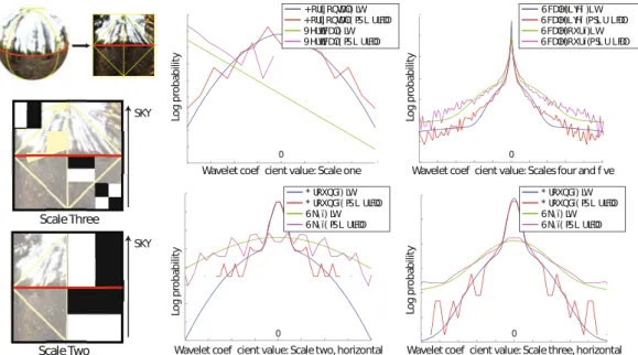
In their work Lombardi et al. [LN12] compare to the previous work of Romeiro et al [RZ10]. The latter gets as input a rendered sphere under an unknown illumination and ex-tracts a monochromatic BRDF. They do not extract the lighting environment which restricts its use to re-use the BRDF under a different environment and forbids the manipulation of the input image. Similar to the work of Lombardi they use priors on natural lighting, in this case they study statistics of a set of environment maps projected in the Haar wavelet

(23)

2.2. Inverse rendering

(1)

(2)

(3)

(a)

(b)

(c)

(d)

Figure 2.4: Results of the alum-bronze material under three lighting environments using Lombardi et al. [LN12] method. Column (a) shows the ground truth alum-bronze material rendered with one of the three lighting environments, column (b) shows a rendering of the estimated BRDF with the next ground truth lighting environment, column (c) shows the estimated illumination map and column (d) shows the ground truth illumination map. The lighting environments used were Kitchen (1), Eucalyptus Grove (2), and the Uffizi Gallery(3). The recovered illumination is missing high frequency details lost at rendering.

. . . . . . Lo g p ro b ab ili ty

Wavelet coef cient value: Scale one

Lo g p ro b ab ili ty Lo g p ro b ab ili ty Lo g p ro b ab ili ty

Wavelet coef cient value: Scales four and f ve

Wavelet coef cient value: Scale two, horizontal Wavelet coef cient value: Scale three, horizontal SKY Scale Three Scale Two . . SKY * URXQGï) LW * URXQGï( PSL ULFDO 6N\ ï) LW 6N\ ï( PSL ULFDO * URXQGï) LW * URXQGï( PSL ULFDO 6N\ ï) LW 6N\ ï( PSL ULFDO 6FDOH)LYHï )LW 6FDOH)LYHï (PSL U LFDO 6FDOH)RXUï)LW 6FDOH)RXUï(PSL U LFDO +RUL] RQWDOï) LW

+RUL] RQWDOï( PSL ULFDO 9HUWLFDOï) LW 9HUWLFDOï( PSL ULFDO

0 0

Figure 2.5: Left: lighting is represented using a Haar wavelet basis on the octahedral do-main discretized to 32 × 32. Statistics of wavelet coefficients are non-stationary, so distinct distributions for coefficients above and below the horizon are fitted. Right: Empirical dis-tributions and their parametric fits for a variety of wavelet coefficient groups.

(24)

basis, see Figure2.5. Those statistics are used to find the most likely reflectance under the studied distribution of probable illumination environments. The type of recovered BRDF is defined in a previous work of the same authors [RVZ08]. That work recovers BRDFs using rendered spheres under a known environment map. They restrict BRDFs to be isotropic and they add a further symmetry around the incident plane, which permits to rewrite the BRDF as a 2D function instead of the general 4D function.

Other methods that perform BRDF estimation always require a set of assumptions, such as single light sources or controlled lighting. The work from Jaroszkiewicz [Jar03] assumes a single point light. It extracts BRDFs from a digitally painted sphere using homomorphic factorization. Ghosh et al. [GCP+₀₉_{] uses controlled lighting based on spherical harmonics.}

This approach reconstructs spatially varying roughness and albedo of real objects. It employs 3D moments (in Cartesian space) up to order 2 to recover basic BRDF parameters from a few views. Aittala et al. [AWL13] employs planar Fourier lighting patterns projected using a consumer-level screen display. They recover Spatially Varying-BRDFs of planar objects.

As far as we know there is no algorithm that works in a general case and extracts a manipulable BRDF alongside with the environment lighting. Moreover, as we are interested in the manipulation of appearance in an interactive manner, re-rendering methods are not suitable. A re-rendering process uses costly global illumination algorithms once material and lighting are recovered. In contrast, we expect that manipulation of shading does not require to decouple the different terms involved in the rendering equation. Therefore, we rather apply approximate but efficient modifications directly to shading, mimicking modi-fications of the light sources or the material reflectance. Moreover, all these methods work on photographs; in contrast we also want to manipulate artwork images.

2.3 Pre-filtered lighting

Pre-filtered environment maps [KVHS00] take an environment lighting map and convolve it with a filter defined by a material reflectance. The resulting values are used to shade arbitrary geometries in an interactive process, giving a good approximation of reflections. Distant lighting is assumed, consequently reflected radiance is independent of position. In the general case a pre-filtered environment would be a 5 dimensional function, depending on the outgoing direction ωo, and on the reference frame defined by the normal n and

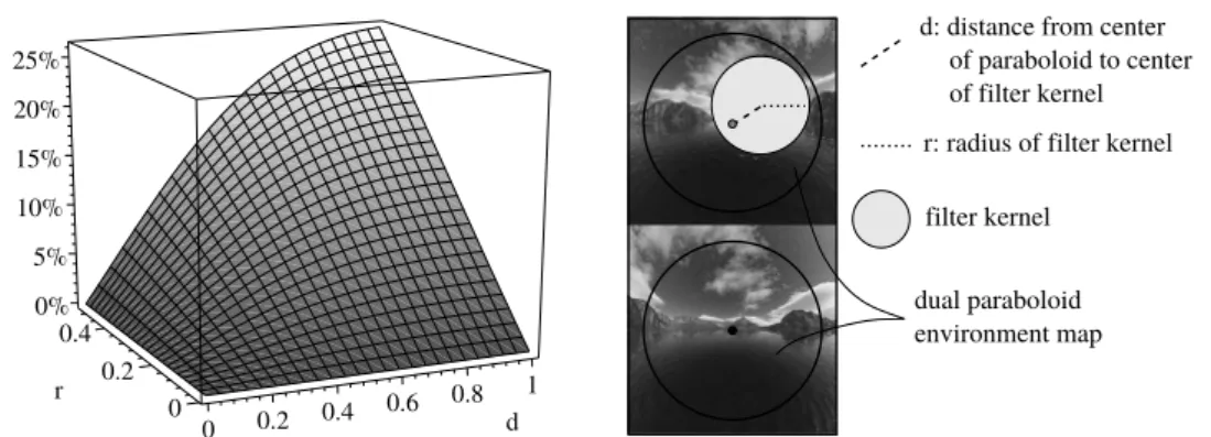
the tangent t. Nevertheless some dependencies can be dropped. Isotropic materials are independent of the tangent space. Radially symmetric BRDFs around either the normal (e.g. lambertian) or the reflected view vector (e.g. Phong) are 2 dimensional functions. When the pre-filtered environment maps are reduced to a 2 dimensional function they can be stored in a spherical maps. A common choice is the dual paraboloid map [HS98], which is composed of a front and a back image with the z value given by 1/2−(x2_+y2_{). This method}

is efficient in terms of sampling and the introduced distortion is small, see Figure2.6. Unfortunately effects dependent on the view direction, like Fresnel, cannot be captured in a single spherical representation as in the last mentioned technique. Nevertheless it can be added afterwards, and several pre-filtered environment maps can be combined with different Fresnel functions. A solution defined by Cabral et al. [CON99] constructs a spare set of view-dependent pre-filtered environment maps. Then, for a new viewpoint they dynamically create a view-dependent filtered environment map by warping and interpolating pre-computed environment maps.

A single view-dependent pre-filtered environment map is useful when we want to have a non expensive rendering for a fixed view direction. Sloan et al. [SMGG01] introduce a technique which creates shaded images of spheres from paintings, which can be used as

(25)

2.3. Pre-filtered lighting 25% 20% 15% 10% 5% 0% r 0.4 0.2 0 _0.4 0.6 0.8 _d1 0.2 0 filter kernel

d: distance from center

dual paraboloid environment map

of paraboloid to center r: radius of filter kernel

of filter kernel

Figure 2.6: Distortion of a circle when projected from a paraboloid map back to the sphere.

(a) Sloan et al. [SMGG01] (b) Todo et al. [TAY13] (c) Bruckner [BG07]

Figure 2.7: Renderings using LitSphere: (a) the original LitSphere technique, (b) a non-photorealistic approach and (c) a technique focused on scientific illustration

view-dependent pre-filtered environment maps (Fig. 2.7a). This technique differs from the previous as it generates shading directly without specifying an environment map and a BRDF. It has been proven useful for non-photorealistic approaches like [TAY13] as well as for technique which convey plausible materials (Fig. 2.7b). The latter is extensively used in sculpting software auch as ZBrush or MudBox, where it is usually called MatCaps (a shorthand for ‘Material Capture”). It has been as well shown useful for scientific illustra-tion [BG07] (Fig.2.7c).

Rammamorthi et al. have shown how diffuse pre-filetered environment maps are well approximated by 9 Spherical Harmonics coefficients [RH01a] corresponding to the lowest-frequency modes of the illumination. It is proven that the resulting values differ on average 1% of the ground truth. For that purpose they project the environment lighting in the first 2 orders of spherical harmonics, which is faster than applying a convolution with a diffuse-like filter. The diffuse color is obtained by evaluating a quadratic polynomial in Cartesian space using the surface normal.

Pre-filtered lighting maps store appearance independently of geometry for distant light-ing. This permits to easily give the same material appearance to any geometry, for a fixed material and environment lighting. As a drawback, when we want to modify the material or the environment lighting they need to be reconstructed, which forbids interactive appear-ance manipulation. In the case of the artwork techniques, LitSpheres/MatCaps are created for a single view, which forbids rotations as shading is tied to the camera.

(26)

2.4 Appearance manipulation

The rendering process is designed to be physically realistic. Nevertheless, sometimes we want to create images with a plausible appearance without caring about their physically correctness. There exist some techniques which permit different manipulations of appearance using different kinds of input, ranging form 3D scenes to 2D images. Those techniques reproduce visual cues of the physically-based image creation techniques but without being restricted by them. At the same time they take advantage of the inaccuracy of human visual system to distinguish plausible from accurate.

Image-based material editing of Khan et al. [KRFB06] takes as input a single image in HDR of a single object and is able to change its material. They estimate both, the geometry of the object, and the environment lighting. Then estimated geometry and environment lighting are used alongside with a new BRDF to re-render the object. Geometry is recovered following the heuristic of darker is deeper. Environment lighting is reconstructed from the background. First the hole left by the object is filled with other pixels from the image, to preserve the image statistics. Then the image is extruded to form a hemisphere. The possible results range from modifications of glossiness, texturing of the object, replacement of the BRDF or even simulation of transparent or translucent objects, see Figure2.8.

Figure 2.8: Given a high dynamic range image such as shown on the left, the Image Based Material Editing technique makes objects transparent and translucent (left vases in middle and right images), as well as apply arbitrary surface materials such as aluminium-bronze (middle) and nickel (right).

The interactive reflection editing system of Ritschel et al. [ROTS09] makes use of a full 3D scene to directly displace reflections on top of object surfaces, see Figure2.9. The method takes inspiration on paintings where it is common to see refections that would not be possible in real life, but we perceive them as plausible. To define the modified reflections the user define constraints consisting on the area where he wants the reflections and another area which defines the origin of the reflections. This technique allows users to move reflections, adapt their shape or modify refractions.

The Surface Flows method [VBFG12] warps images using depth and normal buffers to create 3D shape impressions like reflections or texture effects. In this work they performed a differential analysis of the reflectance radiance Equation (2.1) in image space. From that differentiation of the equation they identify two kind of variations: a first order term related to texturing (variations on material) and a second order variation related to reflection (variations on lighting). Furthermore they use those variations to define empirical equations to deform pixels of an image following the derivatives of a depth buffer in the first case and the derivatives of a normal buffer in the second case. As a result they introduce a set of tools: addition of decal textures or reflections and shading using gradients or images (Fig.2.10).

The EnvyLight system [Pel10] permits to make modifications on separable features of the environment lighting by selecting them from a 3D scene. Users make scribbles on rendered image of the scene to differentiate the parts that belong to a lighting feature from the ones that do not. The features can be diffuse reflections, highlights or shadows. The geometry

(27)

2.4. Appearance manipulation

Figure 2.9: Users can modify reflections using constraints. (a) The mirror reflection is changed to reflect the dragon’s head, instead of the tail. (b) Multiple constraints can be used in the same scene to make the sink reflected on the pot. (c) The ring reflects clearer the face by using two constraints. (d) The reflection of the tree in the hood is modified and at the same time the highlight on the door is elongated.

(a) Brush tool textures (b) Brush tool shading (c) Gradient tool (d) Image tool

Figure 2.10: Tools using Surface Flows. Deformed textures (a) or shading patterns (b) are applied at arbitrary sizes (red contours) and locations (blue dots). (c) Smooth shading patterns are created by deforming a linear gradient (red curve). Two anchor points (blue and red dots) control its extremities. (d) A refraction pattern is manipulated using anchor points. Color insets visualize weight functions attached to each anchor point.

of the zones containing the feature permits to divide the environment map on the features that affect those effect from the rest. The separation of the environment lighting permits to edit them separately as well as to make other modifications like: contrast, translation, blurring or sharpening, see Figure2.11.

Appearance manipulation techniques are designed to help artists achieve a desired ap-pearance. To this end they might need to evade from physical constraints in which computer graphics is based. Nevertheless, obtained appearance might still remain plausible for the human eye. As artists know intuitively that the human visual system is not aware of how light physically interacts with objects.

(28)

original original foreground original background edited edited foreground edited background (a) diffuse (b) highlight (c) shado w

Figure 2.11: Example edits performed with envyLight. For each row, we can see the environ-ment map at the bottom, as top and bottom hemispheres, and the corresponding rendered image at the top. Designers mark lighting features (e.g. diffuse gradients, highlights, shad-ows) with two strokes: a stroke to indicate parts of the image that belong to the feature (shown in green), and another stroke to indicate parts of the image that do not (shown in red). envyLight splits the environment map into a foreground and background layer, such that edits to the foreground directly affect the marked feature and such that the sum of the two is the original map. Editing operations can be applied to the layers to alter the marked feature. (a) Increased contrast and saturation of a diffuse gradient. (b) Translation of a highlight. (c) Increased contrast and blur of a shadow.

2.5 Visual perception

Created or manipulated images are evaluated with respect to a ‘reference’ image (e.g. pho-tograph, ground truth simulation). Measurements of Visual Quality consist in computing the perceived fidelity and similarity or the perceived difference between an image and the ‘reference’. Traditionally numerical techniques like MAE (mean absolute error), MSE (mean square error), or similar have been used to measure signal fidelity in images. They are used because of their simplicity and because of their clear physical meaning. However, those metrics are not good descriptors of human visual perception. In the vast majority of cases human beings are the final consumer of images and we judge them based on our perception. Visual perception is an open domain of research which presents many challenging problems. In computer graphics perception is very useful when a certain appearance is desired, without relying completely on physical control. A survey of image quality metrics from traditional numeric to visual perception approaches is provided in [LK11].

(29)

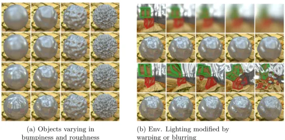
2.5. Visual perception Ramanarayanan et al. [RFWB07] have shown how the human visual system is not able to perceive certain image differences. They develop a new metric for measuring how we judge images as visually equivalent in terms of appearance. They prove that we are not mostly able to detect variations on environment lighting. Users judge the equivalence of two objects that can vary in terms of bumpiness or shininess, see Figure 2.12. Objects are rendered under transformations (blurring or warping) of the same environment lighting. The results prove that we judge images as equivalent, despite their visual difference. This limitation of the human visual system is used in computer graphics to design techniques of appearance manipulation, like shown in the previous section.

(a) Objects varying in bumpiness and roughness

(b) Env. Lighting modified by warping or blurring

Figure 2.12: (a) Objects varying in bumpiness from left to right and the roughness of the material increase vertically. (b) Environment lighting map is blurred in the upper image and warped in the bottom row.

Despite the tolerance of the human visual system to visual differences we are able to dif-ferentiate image properties of objects. To distinguish the material of an object we use visual cues like color, texture or glossiness. The latter is often defined as the achromatic compo-nent of the surface reflectance. In a BRDF, gloss is responsible for changes in the magnitude and spread of the specular highlight as well as the change in reflectance that occurs as light moves away from the normal toward grazing angles. Hunter [Hun75] introduced six visual properties of gloss: specular gloss, sheen, luster, absence-of-bloom, distinctness-of-image and surface-uniformity. He suggests that, except for surface-uniformity, all of these visual properties may be connected to reflectance (i.e., BRDF) properties. There exists standard test methods for measuring some of these properties (such as ASTM D523, D430 or D4039). The measurements of Hunter as well as the standard methods are based on optical measurements of reflections. However, perceived glossiness does not have a linear rela-tionships with physical measurements. The work of Pellacini [PFG00] re-parametrized the Ward model [War92] to vary linearly in relation to human perceived glossiness. Wills et al. [WAKB09] performs an study from the isotropic BRDF database of MERL. From them they create a 2D perceptual space of gloss.

Moreover, perceived reflectance depends on the environment lighting around an object. The work of Doerschner et al. [DBM10] tries to quantify the effect of the environment lighting on the perception of reflectance. They look for a transfer function of glossiness between pairs of BRDF glossiness and environment lighting. Fleming et al. [FDA03] perform a series of experiments about the perception of surface reflectance under natural illumination. Their experiments evaluate how we perceive variation on specular reflectance and roughness of a

(30)

material under natural and synthetic illuminations, see Figure2.13. Their results show that we estimate better material properties under natural environments. Moreover they have tried to identify natural lighting characteristics that help us to identify material properties. Nevertheless, they show that our judgment of reflectance seems to more related to certain lighting features than to global statistics of the natural light.

(a) Materials vary on roughness and specularity

Beach Building Campus

Eucalyptus Grace Kitchen

Point Sources Extended Source White Noise

(b) Natural or analytical environment lighting

Figure 2.13: (a) Rendered spheres are shown by increasing roughness from top to bottom, and by increasing specular reflectance from left to right. The scale of these parameters are re-scaled to fit visual perception as proposed by Pellacini et al. [PFG00] All spheres are rendered under the same environment lighting Grace. (b) Rendered spheres with the same intermediate values of roughness and specular reflectance are rendered under different environment maps. The first two columns use natural environment lighting, whether the last column use artificial analytical environment lighting.

As we have seen the perception of gloss has been largely studied [CK15]. However, we believe that explicit connections between physical and visual properties of materials (independently of any standard or observer) remain to be established.

2.6 Summary

Work on visual perception shows how humans are tolerant to inaccuracies in images. The hu-man visual system may perceive as plausible images with certain deviations from physically correctness. Nevertheless we are able to distinguish material appearance under different illuminations, despite the fact that we are not able to judge physical variations linearly. Manipulation appearance techniques take advantage of these limitations to alter images by overcoming physical restrictions on rendering while keeping results plausible. We pursue a similar approach when using techniques like pre-filtered environment maps, where shading is pre-computed as the interaction of lighting and material. We aim to manipulate dynam-ically geometry-independent stored shading (similar to pre-filtered environment maps) and be able to mimic variations on lighting and material within it. The use of these structures seems a good intermediate alternative to perform appearance modification in comparison to the generation of images using a classical rendering pipeline.

(31)

(32)

Chapter 3 Statistical Analysis

The lightness and color (shading) of an object are the main characteristics of its appearance. Shading is the result of the interaction between the lighting and the surface reflectance properties of the object. In computer graphics lighting-material interaction is guided by the reflected radiance equation [Kaj86], explained in Section2.1:

Lo(x, ωo) =

Z

Ω

fr(x, ωo, ωi) Li(x, ωi) ωi· n dωi ,

Models used in computer graphics that define reflectance properties of objects are not easily connected to their final appearance in the image. To get a better understanding we perform an analysis to identify and relate properties between shading on one side, and material reflectance and lighting on the other side.

The analysis only considers opaque materials which are are well defined by BRDFs [Nic65], leaving outside of our work transparent or translucent materials. We consider uniform ma-terials, thus we only study variations induced by the viewing direction. When a viewing direction is selected the BRDF is evaluated as 2D function, that we call a BRDF slice. In that situation the material acts a filter of the incoming lighting. Our goal is to characterize the visible effect of BRDFs, and how their filtering behavior impacts shading. For that purpose we perform an analysis based on statistical properties of the local light-material interaction. Specifically, we use moments as quantitative measures of a BRDF slice shape.

Moments up to order can be used to obtain the classical mean and variance, and the energy as the zeroth moment. We use those statistical properties: energy, mean and variance to describe a BRDF slice model. In addition we make a few hypothesis on the BRDF slice shape to keep the model simple. Then, this model is used to develop a Fourier analysis where we find relationships on the energy, mean and variance between material/lighting and shading.

Finally we use our moment-based approach to analyze measured BRDFs. We show in plots how statistical properties evolve as functions of the view direction. We can extract common tendencies of different characteristics across all materials. The results verifies our previous hypothesis and show correlations among mean and variance.

This work have been published in the SPIE Electronic Imaging conference with the collaboration of Laurent Belcour, Carles Bosch and Adolfo Mu˜noz [ZBB+₁₅_{]. Specifically,}

Laurent Belcour has helped with the Fourier Analysis, meanwhile Carles Bosch has made fittings on the measured BRDF analysis.

(33)

3.1. BRDF slices

3.1 BRDF slices

When we fix the view direction ωo at a surface point p a 4D BRDF fr is restricted to a

2D BRDF slice. We define it as scalar functions on a 2D hemispherical domain, which we write frωo(ωi) : Ω → R, where the underscore view direction ωo indicates that it is fixed,

and R denotes reflectance. Intuitively, such BRDF slices may be seen as a filter applied to the environment illumination. We suggest that some statistical properties of this filter may be directly observable in images, and thus may constitute building blocks for material appearance.

3.1.1 View-centered parametrization

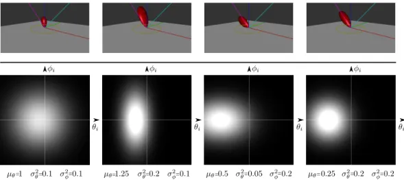
Instead of using a classical parametrization in terms of elevation and azimuth angles for Ω, we introduce a new view-centered parametrization with poles orthogonal to the view direction ωo, see Fig. 3.1. This parametrization is inspired by the fact that most of the energy of

a BRDF slice is concentrated around the scattering plane spanning the view direction ωo

and the normal n, then it minimize distortions around this plane. It is also convenient to our analysis. First, it permits to define a separable BRDF slice model, which is useful to perform the Fourier analysis separately per coordinate, see Section 3.2. Second, it enables the computation of statistical properties by avoiding periodical domains, see Section 3.3. Formally, we specify it by a mapping m : [-π

2,

π

2]

2

→ Ω, given by:

m(θ, φ) = (sin θ cos φ, sin φ, cos θ cos φ), (3.1) where φ is the angle made with the scattering plane, and θ the angle made with the normal

in the scattering plane.

(a) Parametrization isolines (b) Parametrization angles (c) 2D BRDF slice

Figure 3.1: (a) Our parametrization of the hemisphere has poles orthogonal to the view direction ωo, which minimizes distortions in the scattering plane (in red). (b) It maps a pair

of angles (θi, φi) ∈ [−π2,π2] 2

to a direction ωi ∈ Ω. (c) A 2D BRDF slice frωo is directly

defined in our parametrization through this angular mapping.

The projection of a BRDF slice into our parametrization is then defined by:

frωo(θi, φi) := fr(m(θo, φo), m(θi, φi)), (3.2)

where θo, φoand θi, φi are the coordinates of ωoand ωirespectively in our parametrization.

In the following we consider only isotropic BRDF which are invariant to azimuthal view angle. This choice is coherent with the analysis of measured BRDFs as the MERL database only contains isotropic BRDFs. Then, BRDF slices of isotropic materials are only dependent on the viewing elevation angle θo; we denote them as frθo.

Real-time 2D manipulation of plausible 3D appearance using shading and geometry buffers

HAL Id: tel-01440828

https://hal.inria.fr/tel-01440828

Submitted on 19 Jan 2017

HAL is a multi-disciplinary open access

archive for the deposit and dissemination of

sci-entific research documents, whether they are

pub-lished or not. The documents may come from

teaching and research institutions in France or

abroad, or from public or private research centers.

L’archive ouverte pluridisciplinaire HAL, est

destinée au dépôt et à la diffusion de documents

scientifiques de niveau recherche, publiés ou non,

émanant des établissements d’enseignement et de

recherche français ou étrangers, des laboratoires

publics ou privés.

Real-time 2D manipulation of plausible 3D appearance

using shading and geometry buffers

Carlos J. Zubiaga

To cite this version:

Carlos J. Zubiaga. Real-time 2D manipulation of plausible 3D appearance using shading and geometry

buffers. Graphics [cs.GR]. Université de Bordeaux, 2016. English. �tel-01440828�

THESIS

PRESENTED AT

UNIVERSIT´

E DE BORDEAUX

´

ECOLE DOCTORALE DE MATHMATIQUES ET

D’INFORMATIQUE

par

Carlos Jorge Zubiaga Pe˜

na

POUR OBTENIR LE GRADE DE

DOCTEUR

SP´

ECIALIT´

E : INFORMATIQUE

Real-time 2D manipulation of plausible 3D appearance

using shading and geometry buffers

Contents

Chapter 1

Introduction

1.1

Context

1.1.1

Painting

1.1.2

Rendering

1.1.3

Compositing

1.1.4

Summary

1.2

Problem statement

+

=

+

=

1.3

Contributions

Chapter 2

Related Work

2.1

Shading and reflectance

2.2

Inverse rendering

(1)

(2)

(3)

(a)

(b)

(c)

(d)

2.3

Pre-filtered lighting

2.4

Appearance manipulation

2.5

Visual perception

2.6