Calculation of thermal conductance based on measurements of heat flow rates in a flat roof using heat flux transducers

Publisher’s version / Version de l'éditeur:

ASTM Special Technical Publication, 885, pp. 184-202, 1985

READ THESE TERMS AND CONDITIONS CAREFULLY BEFORE USING THIS WEBSITE. https://nrc-publications.canada.ca/eng/copyright

Vous avez des questions? Nous pouvons vous aider. Pour communiquer directement avec un auteur, consultez la première page de la revue dans laquelle son article a été publié afin de trouver ses coordonnées. Si vous n’arrivez pas à les repérer, communiquez avec nous à PublicationsArchive-ArchivesPublications@nrc-cnrc.gc.ca.

Questions? Contact the NRC Publications Archive team at

PublicationsArchive-ArchivesPublications@nrc-cnrc.gc.ca. If you wish to email the authors directly, please see the first page of the publication for their contact information.

NRC Publications Archive

Archives des publications du CNRC

This publication could be one of several versions: author’s original, accepted manuscript or the publisher’s version. / La version de cette publication peut être l’une des suivantes : la version prépublication de l’auteur, la version acceptée du manuscrit ou la version de l’éditeur.

Access and use of this website and the material on it are subject to the Terms and Conditions set forth at

Calculation of thermal conductance based on measurements of heat

flow rates in a flat roof using heat flux transducers

Hedlin, C. P.

https://publications-cnrc.canada.ca/fra/droits

L’accès à ce site Web et l’utilisation de son contenu sont assujettis aux conditions présentées dans le site LISEZ CES CONDITIONS ATTENTIVEMENT AVANT D’UTILISER CE SITE WEB.

NRC Publications Record / Notice d'Archives des publications de CNRC:

https://nrc-publications.canada.ca/eng/view/object/?id=69460ac9-6eed-44cb-8547-fa903dd51def

https://publications-cnrc.canada.ca/fra/voir/objet/?id=69460ac9-6eed-44cb-8547-fa903dd51def

Ser

/E;oYS

THI

Nathal Research _{Council Canada} Conseil _de

_mhemhes

national _Canada

N21d

no

1351

Division of Division des

Building Research recherche en Mtiment c.

2

BIlDG

- - - ---

Calculation of Thennal

Conductance Based on

Measurements of Heat Flow

Rates in a Flat Roof Using

Heat Flux Transducers

by C.P. Hedlin

AT\IALYZ&D

Re~rinted from

"Buildin Applications of Heat Flux Transducers" ASTM. !?TP 885. 1985

p. 184 -202

(DBR Paper No. 1351)

Price $2.00 NRCC 25350

On a mesure, ?i l l a i d e d e t r a n s d u c t e u r s d e f l u x d e c h a l e u r , l e f l u x d e c h a l e u r t r a v e r s a n t un i s o l a n t r i g i d e e n f i b r e m i n e r a l e d e 60 mm d 1 6 p a i s s e u r p o s e d a n s l e t o i t p l a t d ' u n e i n s t a l l a t i o n e x t g r i e u r e d ' e s s a i . Les d i f f d r e n c e s d e t e m p e r a t u r e e n d i v e r s p o i n t s de l ' i s o l a n t o n t Btk mesurees s i m u l t a n e m e n t a u moyen de theymocouples. On a u t i l i s e t r o i s mCthodes a n a l y t i q u e s pour c a l c u l e r l a c o n d u c t a n c e t h e r m i q u e d e l ' i s o l a n t : a ) l e r a p p o r t e n t r e l e f l u x d e c h a l e u r e t l a d i f f e r e n c e d e t e m p g r a t u r e ; h ) l e t a u x d e v a r i a t i o n du f l u x d e c h a l e u r e n f o n c t i o n de l a d i f f e r e n c e d e t e m p e r a t u r e e t d e l a t e m p e r a t u r e moyenne; e t - - - ~- C ) 1~ On compa l e s

.

L ' a u t e u ~ c e q u i s e prod1 d q u e . -

Copyright

Charles

P.

Hedlin

American Society for Testing and Materials _{191 6 Race Street, Philadelphia, PA 19103}

I 1985

Calculation of Thermal Conductance

I

I

Based on Measurements of Heat

!

_{Flow Rates in a Flat Roof Using}

i

Heat Flux Transducers

REFERENCE: Hedlin, C. P., "Calculation of Thermal Conductance Based on Measure- ments of Heat Flow Rates in a Flat Roof Using Heat Flax Transducers," Building Appli- cations offfeat Flux Transducers. ASTM S T P 885, E. Bales, M. Bomberg, and G. E. Courville, Eds., American Society for Testing and Materials, Philadelphia, 1985, pp. 184-202.

ABSTRACT: Heat flow rates through 60-mm-thick rigid mineral fiber insulation mounted in the flat roof of an outdoor test facility were measured with heat flux transduc- ers. The temperature differences across the insulation were measured simultaneously with thermocouples.

Three different analytical procedures were used to calculate the thermal conductance of the insulation:

(a) the ratio of heat flow rate to temperature difference,

( b ) the slope of heat flow rate as a function of temperature difference and mean temper- ature, and

(c) transfer functions.

The results obtained with these three methods are compared.

The effect of ignoring thermal lag was estimated for the first two methods. KEY WORDS: heat flux transducers, flat roofs, thermal insulation, transfer functions, thermal lag, thermal conductance, heat flow

Nomenclature

A Thermal conductance at O°C, W / m 2

-

K

OC Temperature

C Thermal conductance

'Officer in charge, Prairie Regional Station. Division of Building Research. National Re- search Council of Canada. Saskatoon, Saskatchewan 57N OW9. Canada.

HEDLlN ON HEAT FLOW RATES IN A FLAT ROOF 185

I

Thermal conductance found by ratio, slope. and transfer func- _I tion methods

Coefficient representing the variation in thermal conductance

1

with mean insulation temperature, W / m ' . K 2

1

Scanning frequency Heat flow rate. W / m 2

Temperatures at the top and bottom surfaces of the insulation, respectively, O C

Temperature difference across insulation, T H - T 7 . K Mean insulation temperature, ( T T

+

T s ) / 2 , O C

Transfer coefficients for T T , T B , and

Q

The field measurement of heat flow through building envelopes using heat flux transducers (HFTs) is characterized by a variety of conditions and re- quirements.

1. The heat flow varies continuously and unpredictably because of changes in the temperature difference and thermal storage effects.

2. The conditions in normal buildings are not ideal; there may be anoma- lies in the system, such as moisture, discontinuities in thermal insulation, and heat flow diversion by structural members. These cause special problems for measurement and analysis of data.

3. The measurement system should impose the least possible disturbance on the heat flow and, in some cases, moisture movement.

4. The data should be in a form that can be readily handled. Further, the analysis of heat flow data must produce results that have counterparts in the better established steady-state technology.

5. Highly conductive materials are unfavorable for HFT mounting sites; wide temperature swings should be avoided; some heat flux transducers are damaged by moisture. Thus, the choice of the site for an HFT may represent a compromise between the least unfavorable conditions and may require the purchase of heat flux transducers that are appropriate for the circumstances, for example, wet conditions.

This report contains a brief description of a field-type measurement system that is subject, in some degree, to all of the foregoing conditions. It also deals with some aspects of data analysis in which heat flow rates and temperature differences are used to estimate thermal conductance of insulation in sitrr.

Instrumentation

At the Prairie Regional Station (PRS), heat flow has been measured in flat roofs, using one make of heat flux transducer [I]. Two sizes (50 and 106 mm in diameter) were used. These transducers were calibrated by the manufac-

turer and recalibrated at intervals at the Division of Building Research, Ot- tawa, Canada.

I

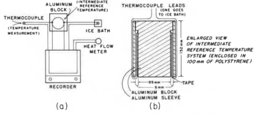
Type-T thermocouples were used to measure temperature. The thermocou- ple was referenced to an aluminum block 89 mm in diameter and 152 mm long, embedded in thick insulation to keep it at a uniform, though not con- stant, temperature. In turn, this block was referenced to an automatic ice bath using a single thermocouple (Fig. 1). Thus, by adding millivoltages, each thermocouple was referenced to the ice point.

I

The output from the heat flux transducers and thermocouples was re- corded by a digital data acquisition system, and the data were processed by

I

computer.

The examples used in this paper are based on data obtained using a speci- men of dry rigid glass fiber 60 mm thick, sealed in polyethylene.

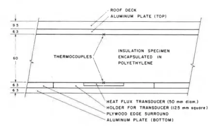
The assembly is shown in Fig. 2. The supporting equipment consisted of two aluminum plates, each 400 mm square and 6.3 mm thick. One plate was secured to the underside of a 9.5-mm-thick plywood roof deck. The heat flux transducer was placed in a 6.3-mm-thick Bakelite holder machined to receive it. The exposed surface of the transducer was flush with the surface of the holder. The holder and transducer were placed on the lower aluminum plate. Plywood 6.3 mm thick was used as edge surround material. The insulation was clamped between the transducer/holder/plywood surface and the upper aluminum plate.

The holder and aluminum plate act as buffers against fluctuations in air temperature. With an unprotected transducer, air movements across the sur- face produce small variations in temperature. Because the temperature drop across the transducer is small, even minor disturbances in its surface temper- ature produce considerable "noise" in its output.

The thermocouples were located a t the top and bottom surfaces of the insu- lation (inside the polyethylene) above the center of the heat flux transducer.

I l N l E R M E D l A T E REFERENCE M E 4 S U R E M E N T I

-

RECORDER THERMOCOUPLE LEADS I O N E GOES

1

1

TO ICE BATH) ENLARGED VIEW OF INTERMEDIATE REFERENCE TEMPERATURE SYSTEM (ENCLOSED IN IOOmm OF POL YSTYffENEl

ALUMINUM BLOCK

( a

( b )

HEDLIN ON HEAT FLOW RATES IN A FLAT ROOF 187 , R O O F DECK

i

/,, A L U M I N U M PLATE ( T O P ) 9 5 / / '

I

6 3

/

I N S U L A T I O N SPECIMEN THERMOCOUPLES, ENCAPSULATED I N

\

POLYETHYLENE I \

i

H E A T FLUX T R A N S D U C E R (50 mm d i a m . ) HOLDER FOR T R A N S D U C E R (125 m m s q u a r e )

FIG. 2-Hoq/cross srcriotrs slrou-itrp locorrotrs o/ hcnur fl,/x mrrrsdricers /dittre~rsiu~rs 111 trrilli- ttrrrrusl.

The heat flow rates and temperatures were measured once every 20 min from January to June. Similar measurements have been made for other insulation specimens, but inclusion of more than one set of results was not considered necessary for the purposes of this discussion.

The temperature of the heat flux transducer varied with daily and seasonal temperature swings. The maximum daily average temperature difference, from winter to summer, was approximately 10 K . Since the HFT output is affected by temperature, a correction based on a laboratory calibration was applied to nullify the effect of this temperature variation.

The results were obtained in the Canadian prairie climate. References to winter and summer are made in that context, and conclusions drawn about daily or seasonal variations may not apply to other regions.

1

Calculation of Thermal Conductance

Three methods of calculating thermal conductance are discussed: (1) a ra- tio method, (2) a slope method, and (3) transfer functions. These are desig- nated C,, C , , and C , , respectively.

Ratio Method

For the ratio and slope methods. daily average values of heat flow rate, Q(W/m2) and AT = T B - T T (where T e and T T are bottom surface and top

The daily averaging method to find

T H ,

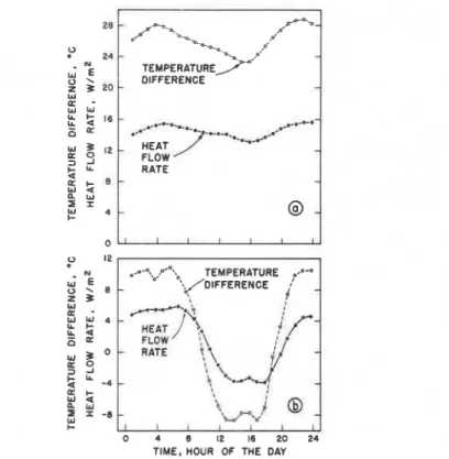
T T , and Q is based on the premise that there are diurnal repetitions of the heat flow and temperature conditions and that thermal mass effects are nullified by the averaging over a full cycle. In fact, a 24-h period does not normally produce closure of the cycle, nor is any other extended or shortened "day" likely to produce an exact repetition of conditions. Presumably, an interval selected so that A T or Q are the same at the beginning and end would be somewhat better in this respect than a fixed 24-h period. Each of these values represents one of the conditions describing the thermal state of the system. If one (or both) are equal at the beginning and end of the test period, other thermal conditions, such as temperature distri- bution, should also be closer to those of the initial state than would be the case at the end of an arbitrarily fixed 24-h period.

Nonclosure and thermal lag are illustrated in Fig. 3. The heat flow rate and temperature difference across the glass fiber specimen versus time of day are

.shn..*. .=..a %..& .o' .-. ,o' TEMPER A T u R E y ' DIFFERENCE f l & - - ~ % / - ] FLOW RATE

0

TEMPERATURE ;eO-'

-

'.;(DIFFERENCE

-

RATE

TIME, HOUR OF THE DAY

FIG. 3- hour!^ tmlperarure differerlces. in dexrees Celsius. and heut flow rutes, in wutls per square ritrtre. for ( a ) u winter duy urld (b) a summer dqv.

HEDLIN ON HEAT FLOW RATES IN A FLAT ROOF ₁₈₉

I

plotted. using 24 of the 72 available values, for a winter day (Fig. 30) and for a

summer day (Fig. 3 1 7 ) . Both sho\t- a 24-h cycle. The daily variation is more pronounced for the summer day than for the winter one. Under some winter conditions. the cycle variation is hidden by long-term changes in tempera- ture; the temperature difference at a selected time of day would not be re- peated in the following 24-h period-and possibly not for a number of days if the temperature continued to drift in one direction. In summer the diurnal swing is normally so large that points somewhere in the cycle are almost cer- tain to be repeated.

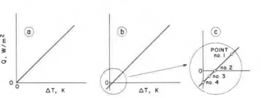
Q can be plotted against A T (Fig. 4). Conductance can be found as the ratio

As

Q

and A T decrease. the error in conductance tends to increase, since mea- surement errors comprise increasingly large fractions of the measured values. Figure 4b illustrates a curve that does not pass through the origin. An ex- panded graph. showing the region of the origin (Fig. 4c), demonstrates that a conductance calculated using Q / A T for Point 1 would give a plausible, but inaccurate, conductance value. At Point 2, the calculated conductance would be zero. at Point 3 it would be negative, and at Point 4 it would be infinitely negative. For data points lying to the left of the origin, conductances will be positive.

A consistent bias in the location of the curve with respect to the origin would occur if there were systematic errors. Such errors might stem from a variety of sources.

Systematic errors would occur if the measurement of temperature differ- ence was consistently inaccurate. In this work, thermocouples were used. Comparison with a calibrated wire-wound resistance thermometer indicated that the thermocouples agreed to within 0.01 K. They were referenced to the

0

/-

---

I

AT, K

aluminum block; hence (assuming that the temperature of the block was uni- form), the error introduced should be very small.

Heat flux transducers could be biased, so that the output for heat flow in one direction is different from that for the same heat flow rate reversed. Tests on the meters used a t PRS did not reveal a detectable error of this type; how- ever, such an error cannot be ruled out.

The thermal conductance is influenced by mean temperature, T , , where

C = A

+

ET,, (3)

Inward heat flow occurs during the warm part of the day. Therefore, for a given temperature difference, the rate of flow will be somewhat higher than the rate of outward flow, which occurs when the insulation is cooler. This would be expected to produce a negative intercept. Normally this does occur, although in the present case (Eqs 5, 9, and 10). the intercept was slightly positive. Scatter or measurement error may mask the temperature effect.

The existence of a negative (or positive) intercept should be construed as an inadequacy of the measurement and analytical procedures rather than as an apparent contravention of thermodynamic laws.

In the present case, it is discussed because, however precise the measure- ment and analyses, some intercept value is likely to exist in practice and affect the conductances calculated by the ratio

In the case of moist insulation, a much greater (negative) intercept occurs than for dry materials [ 2 ] . It is not practical to include it in this discussion. It is mentioned here only to point out the existence of another factor that may complicate the development of equations to express practical heat transfer relationships.

If a finite intercept is caused by systematic measurement error, the conduc- tance (C, in Eq 1) may be found by applying a correction (equal and opposite to the intercept value) to the heat flow values. The difficulty may also be avoided by using the slope of Q versus the temperature parameter, as dis- cussed in the following section.

The Slope Method

Thermal conductance may be found from the slope of an equation that relates heat flow and temperature difference. Thus, if sufficient data points

HEDLIN ON HEAT FLOW RATES IN A FLAT ROOF 191

are available, an equation relating AT and Q can be found by least squares analysis.

Assuming Q to be a second-order function of AT

This is solved in Eq 5 using the data, without allowance for thermal lag.

This is illustrated in Fig. 5.

if the first term on the right is ignored.

Equation 4 implies that the conductance is a function of A T . In fact, al- though AT may have a secondary effect, it is more appropriate to express it in terms of mean insulation temperature. An alternative relationship explicitly includes the effect of mean temperature, T , .

If it is assumed that

where C is the thermal conductance. and

C = A

+

ET,,, (2)

where A = the thermal conductance. C, at O°C, then

Q = A A T

+

EATT,,, (8)

Constants for Eq 8 are found in the following two ways.

1. Approximately, by multiple regression analysis. This results in a small intercept. The analyses were done using data points representing one-day av- erages. Normally. a number of days' data are averaged. However, one of the purposes of this study is to assess the effect of thermal lag; one-day averages were used to avoid the masking of thermal lag effects that occur when a num- ber of days are averaged. When thermal lag was disregarded

When thermal lag effect was included

For the two analyses, the indexes of determination were 0.9996 and 0.9998, and the standard errors of estimate were 0.118 and 0.082 W / m 2 , respectively.

Thermal conductances can be found either by ratio (C, = Q/A T ) or by slope

(C, = Q/A T). From Eq 9

C, = 0.550

+

0.00158T,,, ( W / m 2 . "C) (12)

From Eq 10

I 2. Alternatively, Eq 8 can be solved by using simultaneous equations.

Based on a solution using 85 data points

Q = 0.55lAT

+

0.0017SATTn, (W/m2) (15)

HEDLlN ON HEAT FLOW RATES IN A FLAT ROOF 193

'She heat flo\v rare can he rcprc\ented a j :I functiol~ 01 the 101) anti hottc~m temperatures using polynomial rclation\hil)\

I.;].

One of thc\c invol\c\ 111c u\c of transfer function\. The heat transfer rate. Q. i \ e \ l ~ r c \ \ c d in term\ 01- ten)- peratures. The time lag effcct i \ accommodated b! inclutling earlier \alr~c.\ of' temperature and heat flo\t rate in the relation\liil).

T h e subscripts 0. 1, and 2 indicate the heat flo\v or temperatures occurring currently o r one o r two time steps earlier. ( A time step might be a n hour I l r ~ t

does not have to be.)

In the present case. the follo\t-ing relationship \\-a5 u\ed

K O , the coefficient for

Q,),

is taken to be unity.

Equation 17 might be described as a 3-3-3 arrangement. since there arc three coefficients each for the top and bottom temperatures and heat flux. Other arrangements were tried. including 5-3-3. 5-2-2. and 4-2-2. These ar- rangements weighted representation in favor of the top surface temperature. which varied more widely and erratically than the bottom surface tenipera- ture a n d heat flux. These did not produce better results. based on internal consistency a n d comparison with Eq 14 (or Eq 16).

Equation 17 contain5 eight coefficients, but ten data sets are required to determine the coefficients (data going back two time rteps are requiretl). In the present case. many data were available. A computer program that could

handle u p to 250 d a t a sets was used to obtain best-fit results. Normally. f a r I fewcr than 250 d a t a sets would be ured.

Usually. 24 d a t a sets per day were used.? These tvcre obtained either by

skipping two out of every three of the available numbers or by averaging three

1

consecutive data sets to obtain I-h values of temperature and heat flux. For-

mally 26. 50. 74 . .

.

data sets were used to find conductances for 1. 2. 3 . .-

day periods.

An almost infinite variety of combinations exist\, given the option\ for numbers of coefficients, size of time steps, numbers of data sets used per day. and so on. Perhaps other arrangements \vould have been better tiIan those that were used.

'Thi\ n a \ found to be a \uflicient number of point\. H ~ ~ u e v c r , if letrcr point\ :Ire to Iw u\cd

The transfer function approach is appropriate only for linear systems. A

linear relationship between heat flow and temperature can be derived and

used in Eq 17. It produces a modified expression for temperature which in-

corporates the effect of temperature on thermal conductance. The resulting

conductances should all be equal to the conductance at T,,, = O°C.

The development is as follows

and

where T ; = T T

+

(E/2A)( T:) is a modified temperature, and Q is a linear

function of the modified temperature. Equation 17 then becomes

Using the coefficients in Eq 16

The transfer function coefficients differ widely, depending on the data

used. Table la and b gives four examples based on time steps of 1 h using E /

2A = 0.0016 K-I to adjust the results to a O°C base.

The value of A (the thermal conductance for T,,, = O°C) was computed

HEDLIN ON HEAT FLOW RATES IN A FLAT ROOF 195

The sums of the I and J coefficients should be equal and opposite in sign; thus, conductance can be found by using one or the other. However. the sums are not exactly the same, and an average of the two should be used. This gives

A = 0.561, which is higher than the expected value of 0.551.

The linearizing procedure should make A independent of temperatures. Values of A were found using all of the data. Linear least squares fits gave the following results for E/2A = 0.0016 K-I

and for E / 2 A = 0.0020 K - I

Thus, the temperature effect was almost eliminated by the linearizing pro- cedure.

Calculations were also made using E/2A = 0. The results are shown in Fig. 6 for two-day spans. The best-fit relationship gave

TABLE la-Transfer coefficients for four time periods in 1979. with heat flow data obtained using dry glass fiber 60 mm thick.

Days lo I I 12 K I K z Jo J t Jz

TABLE lb-Interim calculations for a, based on coefficients in Table l a . - X I

A = - A = - L J

-

40 30 20 10 0

A T . K

FIG. 6-Thern~ul cortducrurrces culculated using the trunsjerfunction. C,, versus the mean irrsrr/ofiorr rmiperuture. T,. E/2A = 0.

where C , is used in place of A to indicate that the data are not linearized. The fit is not good, but it does show an upward trend in conductance with increas- ing T,.

Calculation of C Using Values Obtained Within a One-Day Period

In what follows, the data are used to inspect several factors in terms of their influence on C, = Q / A T computed on the basis of one-day averages.

Three points are considered:

(a) whether or not the effect of thermal lag is significant [ 4 ] ,

(b) whether the "day" should be 24 h or variable and determined by some other criterion, and

( c ) the effect of the scan frequency, F, that is, the number of values used per 24-h period, on the accuracy.

I

HEDLIN ON HEAT FLOW RATES IN A FLAT ROOF 197 There still remains the very important practical ta\k o f mounting a heat flux transducer on a building component and allowing for the time required for the resulting disturbance to settle out. The follo\ving mcthod of calculat- ing was used:

1. Thermal lag-Thc temperature values acre paired with Q values mea- sured three scans (60 min) later (as described earlier).

2. Variable day length-In finding a Q versus AT pair for a day, the com- puter first surveyed 100 scans (each representing 20 min) and found the maxi- mum and minimum values of AT in that interval. The mean value, AT,,, was used as the reference temperature difference For that day. Returning to the beginning of the 100-scan interval. the coniputer progresses until AT crosses

ATo. It begins the averaging process at that point and continues until it

reaches a crossing point one cycle later. In some cases, bobbling of AT pro- duced a very short cycle. The computer program was arranged to ignore .;hart

cycles and normally to produce one pair of points per day. Even so. some sets comprised fewer than 40 and others more than 120 scans.

3. Scanning frequency, F-Using 72 scans per day, calculations were made for all the cases in which 7 2 / F was an integer. Further, at each value of F, all the values were used. that is, for F = 36, one pair of Q versus AT values was found by averaging the 1st. 3rd. Sth,

. . .

71st values and a second pair by averaging the 2nd, 4th. 6th,

. . .

72nd values. Thus, for F = 72, there was 1 pair of values. for F = 36 there were 2 pairs. for F = 24 there were 3. and for

F = 18, 12, 9.

.

.

.

1 there were 4, 6, 8,

.

.

. 72 pairs, respectively.

Effect of Thermal Lag and Day Length on C,

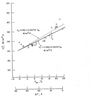
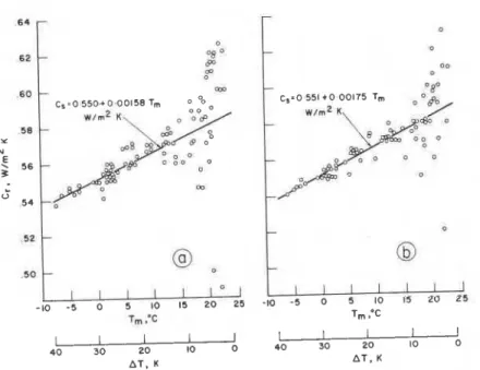
Figure 7 shows conductances ( C , in Eq I ) versus AT (based on one-day averages) along with temperature scales showing T,, and AT. Also included in Fig. 7 is C, (from Eq 12 in Fig. 7a and Eq 14 in Fig. 7b).

In Fig. 7u. no allowance was made for thermal lag, whereas a I -h allowance was made in Fig. 7h. Visual inspection suggests that the inclusion of allow- ance for thermal lag produced a small improvement in the results.

Some comparisons were made using portions of the data. To eliminate ex- treme error values. scans in which the temperature difference was less than 2 degrees Kelvin were left out. Analyses were done for the remaining data ex- clusive of AT

>

12, AT

>

20, and for all the remaining data. that is. the ranges of the three sets of data were 2

<

AT

<

12; 2

<

AT

<

20; and 2

<

AT. This demonstrates the increased error of the estimate of

C,

at reduced

values of AT.

The same process was repeated using variable day length (same AT at the beginning and end). This was limited to cases in which the scan frequency was between 40 and 120, inclusive. The results. including standard errors of esti- mate, are given in Table 2.

T A B L E 2-Standard error (SE. %) in C, based on one-day averages of Q and AT for thermal lag

correctiorrs o f zero and I h."

SE. %

Zero I-h Conditions A T max. O C Lag Lag

72 scanslday 12 4.2 3.0 Fixed A T 12 3.3 3.3 72 scanslday Fixed AT

-

0 0 6 4

-

72 scanslday no limit 2.9 2.0 Fixed A T no limit 2.5 2.4

"Three A T max conditions were used. The calculations for fixed scan frequency and fixed beginning and ending AT. (In the latter case, scan frequencies below 40 and above 120 per "day" were rejected.) A T min = 2°C in all cases.

6 2 0 '3 - P1 m 6 0

-

m2

-

Cs=O 551 t 0 00175 Tm 5%

-

Y N 0 0 0

-

63

- l 1 1 1 ] 1 ~ 52 5 0 -10 -5 0 5 10 I5 2 0 25 -10 -5 0 5 10 15 2 0 25 f m .*C Trn , O C I I I I I I I I I I 4 0 3 0 2 0 10 0 40 30 20 10 0 AT. K AT. K

FIG 7-Plots oJ C, versus T and T,, C , rs based orr one-day averages of Q and T lrtot aN porrrrs are shown) (a) nrthout allowance for therntal lag artd (b) with allowance C, represerzts conductarrce based on the curve of the best frt usrrzg data pornts derrved from 24-h averages rrr Eqs 12 and 14

I

-

-

HEDLIN ON HEAT FLOW RATES IN A FLAT ROOF 199

Using the data in Table 2. the effect of including or ignoring the influence

of thermal lag on C, can be estimated for fixed and variable day lengths. For

the fixed day lengths, the standard error of estimate for C, was reduced by 30

to 35% by including the effect of thermal lag in the computation. For variable

day lengths, there was no apparent reduction when the effect of thermal lag was included.

Comparing standard errors of estimate for fixed versus variable-day

lengths, the standard deviations in C, were not significantly different. Based

on these data and the analytical method used here, using cycles with the same temperature difference at the beginning and end did not appear to improve the result.

Effect of Reduced Scanning Frequency and Thermal Lag on C,

The effect of reduced scanning frequency on C, might be represented in a

variety of ways. In this study, the maximum and minimum values of C , are

found for each value of F

<

72. This difference is divided by 2 and expressed

a s a percentage of the mean value. The mean value is only approximately

correct. Days 26, 137, and 174 are each represented by one point in Fig. 8,

and each of those points lies at some distance from the presumed best value

given by C,.

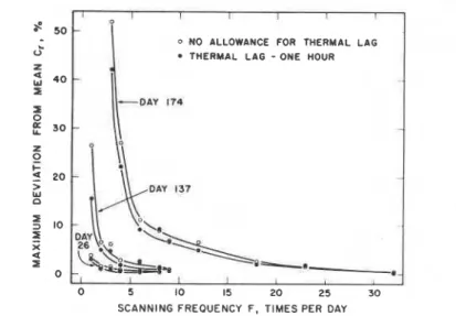
As shown in Fig. 8, the maximum deviation from the mean conductance is

affected by the thermal lag, temperature difference, and frequency of scan-

0 NO ALLOWANCE FOR THERMAL LAG

I

THERMAL LAG

-

ONE HOUR

-

I

0 5 10 15 2 0 2 5 3 0 SCANNING FREOUENCY F. TIMES PER DAY

FIG. 8-Moxirvirrr?~ deviuriorrs of C,frorrr rhr rvieurr vcrlrrrs for rhrrc dirys-scorr firqut,rrcirs

ning. For Day 171. the deviation was very large for low scan frequencies. It decreased rapidly with increasing values of F, reaching 5O/0 for 12 scans per

day and 2 % for 24 scans per day. For Day 137. the pattern was similar. except that a frequency of 4 scans per day reduced the deviation to 3?0 and 2%) for the no-lag and I -h lag calculation.

For Day 26. the maximum deviation from the mean conductance for one scan per day was 4 and 3% for no lag and I-h lag, respectively. and was less than 2% for F = 2 for both cases.

Summary

1 . The study of the thermal performance of buildings may require iir sit11

measurement of thermal conductance of building coniponents. This can be done by analyzing measured heat flow rates and temperatures.

The method of analysis will affect the result. In the present case, simple averaging was used to derive pairs of heat flow and temperature differences for part of the report. Even then, many possibilities exist. The effects of some of these variations were explored using heat flow temperature difference data for a glass fiber specimen. In addition, transfer functions were calculated and used to find thermal conductance.

2. Thermal conductance can be calculated using 24-h average heat flows and temperature differences. This assumes that the thermal conditions in the component being tested repeat themselves every 24 h. This is only approxi- mately correct. In summer a well-defined daily cycle usually occurs, but exact repetition of conditions is unlikely. In winter the cycle is less well defined. Further, because of the thermal inertia of the system, heat flow lags behind the temperature difference that produces it. Scatter in the results is fairly constant for A T greater than 10 K but becomes much larger for A T less than 10 K .

3. Equations representing one-day averages of Q in terms of A T and T,,,

were found with and without correction for thermal lag. Q calculated with the two equations differed by less than 0.04 W / m 2 in the range from 0 to 40°C. Conductance differed by a maximum of 0.75% in the same range. Transfer

I

functions can be used to express the heat flow rate through a specimen as a continuous function of time, given the appropriate temperature conditions applied to the specimen. Also, thermal conductance can be calculated from the transfer functions.

4. Thermal conductance can be defined as the ratio of heat flow rate to the temperature difference, C,, or can be derived from the slope of a second-order relationship between the same two variables, C,. Both have shortcomings. Errors in C, become increasingly large as A T approaches zero. C, can be cal- culated only when sufficicnt data points are available.

5. The effects of thermal lag and scanning frequency on conductances were studied for a winter day, a spring day, and a summer day.

DISCUSSION O N H E A T FLOW RATES IN A FLAT R O O F 201

In a n effort to offset the effects of thermal lag. temperature differences were paired with heat flow rates that occurred 1 h later.

For thermal conductances calculated by the ratio Q i A T . the sn~allest effect of scanning frequency occurred on the winter day. followed by the spring and summer days. The maximum variation from the conductance found by using all 72 values was calculated for scanning frequencies ranging from 72 to 1 per day. Maximum variations were less than 2% for 2 scans on the winter day. for 6 scans on the spring day. and for 24 scans on the summer day. Calculation of the conductances using a thermal lag of 1 h showed reductions in these con- ductance variations ranging up to about 50%.

The author wishes to express his appreciation to Dr. D. G. Stephenson for pointing out a method of showing conductance as a function of mean temper- ature and for assistance in the use of transfer functions. This paper is a con- tribution of the Division of Building Research, National Research Council of Canada, and is published with the approval of the director of the division.

References

111 Hedlin, C. P.. Orr. H. W.. and Tao. 5. S.. "A Method for Determining the Thernial Retis-

tances of Experimental Flat Roof Systems Using Heat Flow Meters." in Thrrr~rol Irrsvluriorr

Perfirr?iunce. ASTM S T P 718. American Society for Testing and Materialr. Philadelphia. 1980, pp. 307-321 (National Research Council of Canada 19274).

121 Hedlin. C. P.. "Effect of Moisture on Thermal Resistance of Some lnsulationr in a Flat Roof

Under Field-Type Conditions." in Therr~rul Ir~srrlrrriorr. Muterirrls. urrd S ~ s r o n r s / h r Errerg>,

Corrservuriorr in the '80s. ASTM S T P 789. American Society for Testing and Materials. Phil- I

adelphia. 1983. pp. 602-625 (National Research Council of Canada 22430). I

131 A.S.H.R.A.E. Hurldbook qf Frrrrdur~rerrruls. American Society for Heating. Refrigerating.

and Air Conditioning Engineers. 1977. Chapter 25.

141 Brown. W . C. and Schuyler. G. D.. "In Situ Measurements of Frame Wall Thermal Resir-

tance."A.S.H.R.A. E. Trurrsucrioris. Vol. 88. Part I . 1982. pp. 667-6761 (National Rewarch

Council of Canada 20851 ).

1

DISCUSSION

D. L. McElroy

'

(writtell discussioi~l-Have you considered radiation trans- fer to explain any of your results?

C. Hedlin (author's closure)-No effort was made to estimate the individ- ual contributions of radiation or other heat transfer modes.

D. A. Hugcln2 (written discussion)-How did the phase shift correction of Q versus T relate to the time constant of the component being tested, and did the resulting calculation of thermal conductivity convert to the same value as the uncorrected calculation?

C. Hedlin luuthor's closure)-In Fig. 3b. the heat flow rate was estimated to lag behind the temperature difference by about 1 h, based on the difference in time as each crossed the line when temperature difference and heat flow rate were zero. The calculations were made pairing temperature differences with simultaneous heat flow rates and also with heat flow rates occurring 1 h later.

Rough comparisons of the results with and without allowance for thermal lag were made for the ratio and slope methods. For the first, Fig. 7 shows that maximum deviations of C, from the mean were somewhat (1 to 5 % ) less when thermal lag was taken into account. For the slope method, a least squares analysis of heat flow versus a combination of temperature difference and mean temperature gave standard errors of estimate of 0.118 and 0.082 W / m 2 when the lag was neglected or considered, respectively. Further, the heat flow rate calculated by comparison of the two equations (Eqs 9 and 10) at several points showed that estimated values of heat flow rate differed by less than 0.05 W/m2. Equations 12 and 14 give the thermal conductances obtained when thermal lag was disregarded and when it was included.

T h i s p a p e r , w h i l e b e i n g d i s t r i b u t e d i n r e p r i n t form by t h e D i v i s i o n of B u i l d i n g R e s e a r c h , remains t h e c o p y r i g h t of t h e o r i g i n a l p u b l i s h e r . I t s h o u l d n o t be r e p r o d u c e d i n whole o r i n p a r t w i t h o u t t h e p e r m i s s i o n of t h e p u b l i s h e r . A l i s t of a l l p u b l i c a t i o n s a v a i l a b l e from t h e D i v i s i o n may be o b t a i n e d by w r i t i n g t o t h e P u b l i c a t i o n s S e c t i o n , D i v i s i o n of B u i l d i n g R e s e a r c h , N a t i o n a l R e s e a r c h C o u n c i l of C a n a d a . O t t a w a , O n t a r i o . K1A OR6. Ce document e s t d i s t r i b u g s o u s forme d e t i r k - a - p a r t p a r l a D i v i s i o n d e s r e c h e r c h e s e n b a t i m e n t . Les d r o i t s d e r e p r o d u c t i o n s o n t t o u t e f o i s La p r o p r i C t 6 d e l l € d i t e u r o r i g i n a l . Ce d o c u m e n t n e p e u t O t r e r e p r o d u i t en t o t a l i t k ou e n p a r t i e s a n s l e consentement d e l ' g d i t e u r . Une l i s t e d e s p u b l i c a t i o n s d e l a D i v i s i o n p e u t S t r e o b t e n u e en 6 c r i v a n t a l a S e c t i o n d e s p u b l i c a t i o n s . D i v i s i o n d e s r e c h e r c h e s e n b a t i m e n t , C o n s e i l n a t i o n a l d e r e c h e r c h e s Canada, Ottawa. O n t a r i o , KIA 0R6.