HAL Id: hal-03138314
https://hal.archives-ouvertes.fr/hal-03138314
Submitted on 11 Feb 2021
HAL is a multi-disciplinary open access
archive for the deposit and dissemination of
sci-entific research documents, whether they are
pub-lished or not. The documents may come from
teaching and research institutions in France or
abroad, or from public or private research centers.
L’archive ouverte pluridisciplinaire HAL, est
destinée au dépôt et à la diffusion de documents
scientifiques de niveau recherche, publiés ou non,
émanant des établissements d’enseignement et de
recherche français ou étrangers, des laboratoires
publics ou privés.
Improving on coalitional prediction explanation
Gabriel Ferrettini, Julien Aligon, Chantal Soulé-Dupuy
To cite this version:
Gabriel Ferrettini, Julien Aligon, Chantal Soulé-Dupuy. Improving on coalitional prediction
explana-tion. 24th European Conference on Advances in Databases and Information Systems (ADBIS 2020),
Aug 2020, Lyon, France. pp.122-135, �10.1007/978-3-030-54832-2_11�. �hal-03138314�
Gabriel Ferrettini, Julien Aligon, and Chantal Soul´e-Dupuy
Universit´e de Toulouse, UT1, IRIT, (CNRS/UMR 5505) [email protected]
Abstract. Machine learning has proven increasingly essential in many fields but a lot obstacles still hinder its use by non-experts. The lack of trust in the results obtained is foremost among them, and has inspired several explanatory approaches in the literature. These approaches pro-vide a great insight on the predictions of a model, but at a cost of a long computation time. In this paper, we aim to further improve the detection of relevant attributes influencing a prediction, on the strength of feature selection methods.
Keywords: Data analysis· Machine learning · Prediction explanation.
1
Introduction
One of the main limits to the use of machine learning solutions is the ”black box” problem inherent to an opaque model, producing results without insight of how they were produced. As an answer to this problem, several methods exist to explain a predictive model, in a global way [1]. A problem arise when a domain expert user (for instance a biologist) has to study the behavior of particular dataset instances over a predictive model (for instance in the context of cohort study). In this case, a global explanation is not enough to give the information needed by the study. In this direction, previous studies offer the possibility of explaining single instance prediction, over a model, as in [14] and [3]. One major problem of these contributions is the high complexity of the proposed algorithms (O(n2)). Because of this computational weight, explaining each instance over a
predictive model can be very time consuming, especially if the dataset has a large number of attributes.
Our work fits the general ambition to help a domain expert user to get involved in data analysis operations, especially in learning tasks. On this way, obtaining explanations for predictive models, in a reasonable time, is essential. In a previous work [5], we proved the feasibility of lowering the computation time of existing solutions, with a very limited loss of explanation accuracy while saving a high computation time. In this paper, we continue this work to find better approximations of these solution, through the exploration of new ways to find groups of attributes.
The paper is organized as follows. Section 2 explores previous works already done in the domain of prediction explanation. In particular, the identification of attributes having a significant influence on a model is fundamental. To that end,
the automated discovery of groups of linked attributes is an important challenge to overcome. Notably, we rely on attribute grouping methods from the literature, notably inspired by the feature selection methods. Then, Section 3 describes the base methods used to generate predictions explanation. The extension of our work [5] is proposed in Section 4 to find faster methods of explanation. This is achieved through new way to find groups of attributes for the coalitional method described in Section 3. Experiments are presented in Section 5, showing the interest of our methods in terms of computation time and their limited impacts in terms of loss of accuracy, significantly improving the results of [5]. Finally, Section 6 concludes the paper by giving new perspective of works, including the new possibilities opened by our results.
2
Related works
Explaining the influence of each attribute (of a dataset) on the output of a pre-dictive model has been explored largely. An example of the works pertaining to global attribute importance on a model is available in [1]. The most recent meth-ods are based on swapping the values of attributes in a dataset and analysing which swap affects the most the predictions trained by a model. The more mod-ifying the attributes values affects the predictions, the most this attribute is considered important for the model, as a whole. Many ways of explaining single predictions have been explored but these methods often struggle between being too simplistic, or too complex to be interpreted by a human, notwithstanding the problem of computation time, which can become problematic for more advanced user assistance systems. The possible applications of prediction explanations are investigated by [11]. According to their paper, the interest for explaining a pre-dictive model is threefold. It can help to (1) understand, (2) judge the quality and (3) choose a model. A great number of works pertaining to prediction ex-planation led to [8], which theorized a category of exex-planation methods, named additive methods, and produced a review of the different methods developed in this category, such as [4] and [13]. These methods provides, for a given predic-tion, a weight to each attribute of the dataset, representing its influence on a model, locally. Different additive methods exist to calculate relevant weights but the end result is always this vector of weights. This vector is easy to interpret, even for someone without expertise on machine learning. Yet, these methods have a major deterrent: their computation time makes them difficult to use for the average user. That is why [8] explores methods to generate explanations faster, but at the cost of very restricting hypotheses, as the independence of each attribute of the dataset, or the linearity of the model, which is not always the case. Thus, we are aiming for a simplification to reduce computational time of methods like [14], but applicable in a more generic way than [8]. In this work, we want to facilitate the generation of prediction explanation, without having to restrict ourselves to a given set of models. This paper is the continuity of [5] in which we already established possible methods of simplification. One of these methods relies on the automatic detection of groups of attributes. In this paper,
we aim to identify and compare additional methods detecting groups, in order to compare their influence on the efficiency of the simplification method.
The selection of relevant attributes to be grouped can take inspiration from the works in the field of feature selection [2] [16]. In particular, the methods proposed in a dimensional reduction goal seem to reach our scope. Indeed, these methods have to automatically detect interactions between attributes for reduc-ing a potential high dimensionality in a dataset. Thus, two main approaches, feature extraction (mainly the principal component analysis) and filter methods (which measure the relevance of features by their correlations) can be considered. The fact that the principal component analysis (PCA) and the filter methods rely only on information provided by a dataset (independent of the model used in an analysis) is a great advantage for our work, in contrast with techniques such as SVM-RFE [10] or FS-P [9], based on a specific model. Indeed, different predictive models can classify differently a same instance. Thus, an explanation on this instance can be different, from one model to another, and cannot depend of a selection of influence attributes made by a unique predictive model, such as SVM. The PCA is a largely recognised method to provide new features from sets of correlated attributes. The Correlation-based feature selection (CFS) methods [6] are promising candidates. In particular, the use of a multicollinearity measure by a variance inflation factor (VIF), can provide sets of attributes having linear correlations between them. This avoids calculating collinearity between pairs of attributes, using the Pearson’s measure, for example. However, the VIF measure is unable to compute non linear correlations, on the contrary of the Spearman correlation factor. Even if this factor only works between pairs of attributes, the capacity to detect non linear correlations makes it a good candidate.
3
Prediction explanation
In this section, we present the basis of our current work : the methods used to generate prediction explanations. First, we introduce our baseline, the com-plete explanation, and then we present our simplification of this baseline, the coalitional explanation.
3.1 Complete explanation
The baseline of our work takes inspiration from the work of [14]. This influence calculation method is based on the computation of attribute influences for all possible subgroups. This framework is close to the situation of a game called ”coalitions”, where each group of attributes can have an influence on the model prediction. The influence of an attribute is measured according to its importance in each coalition. We can then refer to the coalition games as defined by Shapley in [12]: A coalitional game of N players is defined as a function mapping subsets of players to gains g : 2N 7→ R. The parallel can easily be drawn with our
situation, where we wish to assess the influence of a given attribute in every possible coalition of attributes. We then look at not only the influence of the
attribute, but also its use in all subsets of attributes. We thus define the complete influence of an attribute ai ∈ A on the classification of an instance x for the
class C : IC ai(x) = X A0⊆A\a i
p(A0, A) ∗ (inff,(AC 0∪a
i)(x) − inf
C
f,A0(x)) (1)
With p(A0, A) a penalty function accounting for the size of the subset A0. Indeed, if an attribute changes a lot the result of a classifier, in a large group of attributes, it can be considered as very important for the prediction compared to the other ones. On the opposite, an attribute changing the result of a classifier, when this classifier is based on a small set of attributes, cannot be considered to have an influence as decisive as the first one. The Shapley value [12] is a promising candidate, and defines this penalty as:
p(A0, A) = |A
0|! ∗ (|A| − |A0| − 1)!
|A|! (2)
The base influence infC
f,A(x), defined in [14], is the difference between the
prediction without prior information, and the prediction with every attribute in the group of attributes A :
inff,AC (x) = f (xA) − f (∅) (3)
This complete influence of an attribute now takes into consideration its im-portance among all the possible attribute configurations, which is closer to the original intuition behind attribute influence. However, because we ambition to explain a single instance on a model, the complete influence can be extremely computationally expensive: (2n∗ l(n, x)), with n the number of attributes, x
the number of instances in the dataset and l(n, x) the complexity of training the model to be explained It is then not practical to use the complete influence and it becomes necessary to seek a more efficient way. However, the complete influ-ence can be considered as an excellent baseline [14]. Thus, our new explanation approaches can be evaluated by measuring how they deviate from the complete influence.
3.2 Coalitional explanation
A more efficient strategy is to only identify the groups of correlated attributes, as proposed in our previous work [5]. This strategy avoids having to calculate all possible subgroups of influence. We then obtain a coalitionnal influence of an attribute ai∈ g, g ∈ G : simpleIaC i(x) = X g0⊆g\ai p(g0, g) ∗ (inff,(gC 0∪a i)(x) − inf C f,g0(x)) (4)
Given the fact we can set a maximum cardinal c for our subgroups, the complexity is, in the worst case, O(2c∗n
calculates less groups than the complete influence, but tries to make up for it by only grouping the attributes actually related to each other. In order to determine which attribute groups are relevant to consider, we need to use an automatic attribute groups construction method.
4
Coalition computing methods
We propose, in this section, different ways to compute attribute coalitions and study their effects on the efficiency of the coalitionnal influence. We base our first algorithm on the work of [7]. The other algorithms are based on the variance inflation factor (VIF) and the principal component analysis (PCA) of a dataset. For each algorithm, we implement a parameter which control the size of the subgroups that are generated. A higher value of this parameter generates larger groups whereas a smaller value produces smaller groups.
4.1 Model-based coalition
In this method, the attribute groups are created by using the model itself to detect interacting attributes. In this approach, no correlation is detected, but only an interaction in the sense of the model usage of the attributes. This is done by randomizing the values of the dataset, and studying the evolution of the model predictions. It consists in measuring the differences of predictions on the whole dataset before and after the randomization. When attributes are considered to be part of the same group, their values are swapped together with the values of another instance, classified by the model as the same class as the starting instance. Each attribute outside of the group has its value swapped completely randomly. Once this have been done, the new instances are classified by the model. The ratio of differences between the old and the new classification is called the fidelity. A higher fidelity meaning a lower variation of the predictions. At each iteration, the attribute which removal lowers the less the fidelity is removed, until it is not possible to keep the fidelity above a fixed threshold. Then the group is considered as fixed. This attribute grouping algorithm has been developed in [7] and is detailed in Algorithm 1.
4.2 Principal component analysis based coalition
The objective of a principal component analysis is to transform correlated at-tributes into new atat-tributes linearly uncorrelated between them. Our reasoning, for this approach, is to consider the set of correlated attributes (summarized by the new attribute of the PCA) as a group of influence.
Given a dataset D = (A, X) composed of a set of n attributes A = {a1, ..., an},
and a set of instances X where x ∈ X, x = {x1, ..., xn}∀i ∈ [1..n], xi∈ ai.
We can apply a principal component analysis which produces a new dataset D0 = (A0, X0) such as A0 = {a01, ..., a0m} with each new attribute being a linear
Algorithm 1 Model-based coalition extraction
Input: Sensitivity parameter δ > 0, the number of attributes m, and a fidelity function f id(). Two auxiliary functions L(X) =S
i∈X{{i}} and F (X) = L(
S
Y ∈XY ), which
produces sets of singletons (e.g. L({1, 2, 3}) = F ({{1, 2}, {3}} = {{1}, {2}, {3}}) Output: σ a coalition of attributes
σ ← {}
R ← {m} . R contains a group to test for A ← {} . A contains the removed attributes ∆ ← f id(L([m])) + δ
while R 6= {}orA 6= {} do
if A = {} and f id({R}S F (σ)) < ∆ then
. if we are already below ∆ before removing any attribute assign the remaining attributes to singleton groups
σ ← σS L(R) R ← {} A ← {} else
. Find an attribute j whose removal from R decreases the fidelity least j ← argmaxj∈Rf id({{R\{j}}S{{j}} S{A} S F (σ))
if |R| = 1 or f id({{R\{j}}S{{j}} S{A} S F (σ)) then
. If the fidelity drops below ∆ add the group of attributes to the results and look for the next group of attributes
σ ← σS{R} R ← A A ← {} else
. If the fidelity stays above ∆ continue removing the grouping R R ← R\{j} A ← AS{j} end if end if end while return σ
composition of the previous attributes : ∀i, a0i ∈ A0, ∃ {α
1, ..., αn} ∈ Rn, a0i =
α1∗ a1+ ... + αn+ an.
Each new instance is associated with an instance of the previous dataset. ∀x0= {x0
1, ..., x0m} ∈ X0, ∃! x ∈ X, ∀i ∈ [1, .., m]∃ α1, ..., αn∈ Rn, x0i= α1∗ x1+
... + αn+ xn.
Given this set of factors α1, ..., αn, for each attribute, we consider each factor
as an evaluation of the importance of the attributes in the group. We can then constitute a coalition of attributes by exploiting the groups formed by the most important factors. This gives us the algorithm 2. For the sake of simplicity, we consider each a0∈ A0 as a vector of its α
Algorithm 2 PCA-based coalition extraction
Input: a threshold t and the set of attributes A0 of the PCA Output: σ a coalition of attributes
σ ← {}
for all a0∈ A0 do . for each attribute generated by the PCA g ← {} . g, a new possible group αmax ← max(a0= α1, ..., αn) . find the most important factor
for all αi∈ a0 do
if αi≥ α max ∗ (1 − t) then
add ai to g . the attribute is included in the group if close to the max
end if end for add g to σ end for return σ
4.3 Variance Inflation Factor based coalition
The variance inflation factor (VIF) is an estimation of the multicollinearity of the attributes of the dataset in regard to a given target attribute.
Given a dataset D = (A, X), the VIF value of a ∈ A is calculated by running a standard linear regression with a as the target for the prediction. Then, given R the coefficient of determination of the linear regression, we have:
V IF (a) = 1
1 − R2 (5)
It is commonly accepted that a variance inflation factor superior to 10 in-dicates a strong multicollinearity of the attribute with other attributes of the dataset. Moreover, when an attribute is removed from the dataset, the VIF of the attributes multicollinear with it decrease. Then, we can automatically detect groups of attributes by calculating the VIF of each attribute (considered as a target) of the dataset, and then comparing them with a new VIF calculation with an attribute removed. For this purpose, we consider two possible approaches:
– Considering as a priority the calculation of strongly multicollinear groups of attributes: Those are groups of attributes with a dependency to one another. In the context of this approach, attributes whose VIF varies strongly when an attribute is removed from the dataset will be considered as part of the group.
– Considering as a priority the calculation of weakly or non multicollinear groups of attributes: Given the fact that correlated attributes tend to bring the same information to the model, it may be preferable to prioritize groups for which the addition or removal of an attribute will change greatly the information brought by the group.
These two approaches are named VIF coalition and reverse VIF coalition, respectively. This gives us the algorithm 3, for the VIF coalition. The reverse
Algorithm 3 VIF-based coalition extraction
Input: a threshold t, the set of attributes of the dataset A and a function V IF (A) calculating the array of all the VIF of all the subsets of a set of attributes
Output: σ a coalition of attributes σ ← {}
oldvif s ← V IF (A) . calculating the initial VIFs of the attributes for all a ∈ A do
g ← {} add a to g
newvif s ← V IF (A/a) for all a0∈ A do
if newvif s(a0) < oldvif s(a0) ∗ (0.4 + t) then add a0 to g end if end for add g to σ end for return σ
VIF coalition can be obtained simply by replacing the condition for adding an attribute to a group by if newvif s(a0) > oldvif s(a0) ∗ (1 − t ∗ 0.05). This
supplementary ratio of 0.05 have been obtained by preleminary experiments, which showed that just keeping the 1 − t factor led to a generation of all the possible subgroups, which defeat the principle of an approximation.
4.4 Spearman correlation based coalition
A limit of the variance inflation factor is the sole consideration of multicolin-earity, while a correlation between attributes might not be linear. This problem is addressed through the Spearman correlation coefficient, which takes into ac-count non linear correlations. Spearman being not multicollinear, the calculation of the correlation between attributes has to be done by pairs. Thus, the method consists in generating the matrix of all the correlations of each pair, and then deciding which attributes are part of a group. For this method, we have the same two possibilities as for the VIF method: we can either prioritize the calculation of strongly correlated attributes, or on the contrary, prioritize groups of non correlated attributes. These two approaches are named respectively Spearman coalition and reverse Spearman coalition.
Given a dataset D = (A, X), with A = {a1, ..., an} the correlation matrix C
is obtained by computing the spearman correlation coefficient of each attribute couple : C(1, 2) = corr(a1, a2). Thus C is symmetrical and have 1 as the value
of its whole diagonal. For each line i of the matrix C, we consider as grouped with ai the attributes strongly (or weakly) correlated with ai, for the Spearman
coalition (or the reverse Spearman coalition).
The algorithm 4 details the Spearman coalition method. In order to perform the reverse Spearman coalition method can be obtained by replacing the
condi-Algorithm 4 Spearman-based coalition extraction
Input: a threshold t, the set of attributes of the dataset A and a function spearman(A) calculating the matrix of all the absolute spearman correlation coefficient of all the subsets of a set of attributes. a max and min functions which returns the maximum and minimum of a matrix line.
Output: σ a coalition of attributes σ ← {}
corrmat ← spearman(A) . calculating the correlation matrix for all a ∈ A do
g ← {}
for all a0∈ A do
if corrmat(a, a0) > max(corrmat(a)) ∗ (1 − t) and max(corrmat(a)) > 0.1 then
. If the most correlated attribute have a coefficient less than 0.1, we consider a as a singleton add a0 to g end if end for add g to σ end for return σ
tion for adding an attribute to a group by corrmat(a, a0) < min(corrmat(a)) + max(corrmat(a)) ∗ t and min(corrmat(a)) < 0.5. This allows to add the least correlated attributes up to a threshold : if the minimum is superior to 0.5, we consider the attribute as too correlated to the others and consider it as a single-ton.
5
Evaluating the coalition computation methods
In this section we aim to evaluate the performances of each coalition calculation method, considering their precision when compared to the complete influence, and their computational time. We also give an overview of the group character-isation for each coalition method.
5.1 Experimental protocol
Our experiments are run on the OSIRIM1cluster. This cluster is equipped with
4 AMD Opteron 6262HE processors with 16 x 1,6 Ghz cores, for a total of 64 cores, and 10 x 512 GB of RAM. Our tests are realized from the data available on the Openml platform [15]. We select the biggest collection of datasets2on which classification tasks have been run. We also consider six classification tasks: na¨ıve Bayes, nearest neighbors, J34 decision tree, J34 random forest, bagging na¨ıve
1
http://osirim.irit.fr/site/en
2
Bayes and support vector machine. Due to the heavy computational cost of the complete influence (considered as the reference of our experiments), we select the datasets having at most nine attributes. Thus, a collection of 324 datasets is obtained. Considering the six types of workflows, we have a total of 1944 runs. For each of those runs, we generate each type of influence proposed in this paper, for each instance of the 324 datasets: the complete influence for the baseline, along with the coalitional influence. The coalitional influences are generated using the different group generation methods described in Section 4, which are based on an α ∈]0, 0.5[ parameter (small values of α resulting in smaller subgroups, and high values in bigger ones). We generate the possible subgroups with 5 different values of α to study the influence of subgroup size. To compare the different explanation methods, we consider the explanation results as a vector of attribute influences noted I(x) = [i1, ..., in] with n the number of attributes in the dataset.
Thus, each of the attributes ak is given an influence ik ∈ [0, 1] by the method
I : ∀k ∈ [1..n], ik = Iai(x), with x an instance of the dataset. We then define
a difference between two vectors of influences i, j as the normalised euclidian distance: d(i, j) = 1 2√n n X k=1 p (ik− jk)2 (6)
Considering this formula, we define an error score based on the difference between an explanation method and the complete influence method. Given an instance x, an explanation method I(x), and the complete influence method IC(x):
err(I, x) = d(I(x), IC(x)) (7)
For each instance of each dataset, we generate the error score of every method, allowing us to compare their performances across the different collected datasets . Each error score is the distance of one of the coalitional methods from the complete method. Thus, lesser error is indicative of a more precise estimation of the complete method.
5.2 Calculation time and Error scores
Table 1: mean number of instances for datasets with a given number of attributes
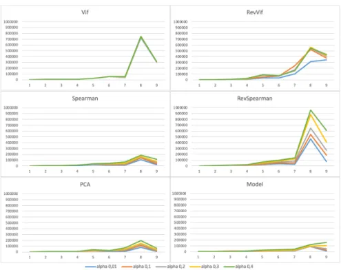
Figures 1 and 2 give the performance and computational time in miliseconds of each coalitional method, respectively (for different values of their threshold parameter).
For readability, Table 1 details the mean number of instances for each number of attributes. This can have an impact on computation time, and explains the variations of Figure 1. This figure includes the computation time for generating the groups of attributes and for explaining each instance of the dataset. The decrease of the computation time for the case of 9 attributes is explained by the important decrease in the mean number of instances. This makes each retraining
Fig. 1: Calculation time of each coalitional method versus the number of at-tributes in the dataset
faster to do, even if there are potentially twice more subgroups to take into account.
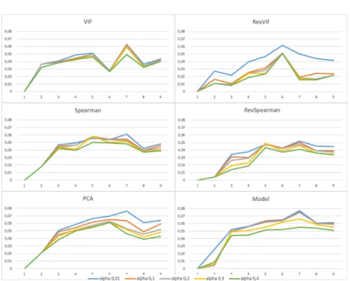
Figure 2 depicts the mean error score, aggregating the error score (Equation 7) of each explanation method for each of our 324 datasets. In this figure, the closer the curve is to 0, the closer it is to the complete influence method.
As we can see, in an overall analysis, the VIF method seems to be the worst, with a poor performance and a long computational time. This can be explained by the fact that the attributes of the generated group are correlated to one another, which mean that the information brought by these groups and subgroups is very redundant. We can suppose a lot of groups are calculated (see Section 5.3 for more details), but they often bring nearly the same information each. Spearman has a far better computation time than VIF, but still has a poor performance overall, probably for the same reasons. As an example, PCA has a better performance but a computation time very similar to Spearman. RevSpearman has an overall better performance than part of other methods, but this performance is paid by the longest computation time, without reaching the best performance. This can be explained by the group calculation method,
Fig. 2: Error score between each coalitional method and the complete influence, versus the number of attributes in the dataset
which does not take into account the possible correlation of two attributes which are both not correlated with the original attribute of the group (no transitivity). This lead, as for VIF and Spearman, to the calculation of redundant information, which increases the computation time without improving much the performance. The PCA, RevVIF, and Model methods each seem to have their strong and weak points. The RevVIF is clearly more precise than the other two, but at a cost of greatly increased computation time. Instead of focusing on the correlated groups, the RevVIF method relies on the least correlated, thus a greater diversity of information is taken into account. While the Model and PCA methods are less exhaustive in their approaches, they seem to have a far lower computational time, the evolution of computation time against the number of attributes being far less steep than for RevVIF.
5.3 Group characterisation
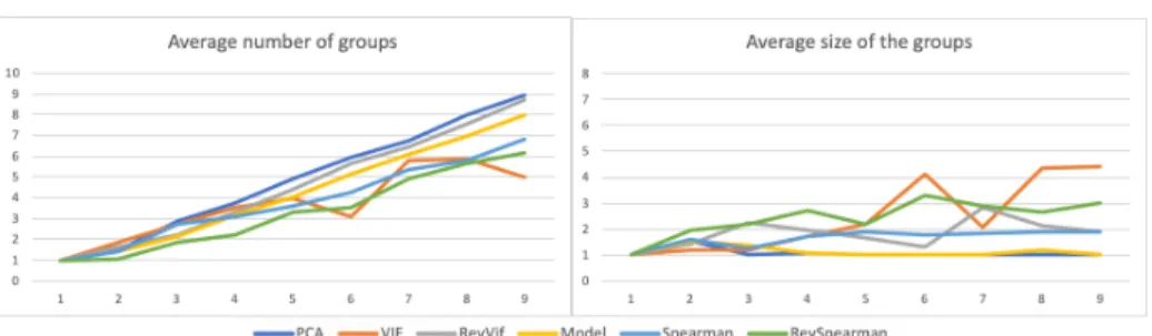
Figures 3 and 4 compare the average number and average size of the groups of attributes generated by each coalitional method, respectively (for the two ends alpha = 0.01 and 0.4).
We can note that RevVIF, RevSpearman and VIF are the three methods generating the highest average group sizes, compared to the other methods. This
Fig. 3: Group characterisation with alpha = 0.01
Fig. 4: Group characterisation with alpha = 0.4
phenomenon can explain why these methods minimize best the error scores as discussed in Section 5.2. Indeed, the larger the groups are, the more exhaustive they are in terms of coalition influence that can correctly explain an instance with respect to a predictive model. More surprisingly, the high average number of groups seem not to induce a good error score. For example, the RevSpearman method generate, for the two alpha thresholds, the lowest number of groups, for most of the cases, whereas its error rate is one of the best. This can be explained by the generation of a lot of small groups (singletons or couples), rather than a few large ones. After all, the complete influence is the equivalent of the coalitional influence using a single group containing all the attributes.
6
Conclusion and perspectives
In this paper, we proposed a comparative study between several attribute group-ing methods (inspired by the feature selection field) in an objective of individual prediction explanation. Our tests, conducted with 324 real datasets, show that RevVIF, PCA and Model methods are all of interest. RevVIF is preferable for datasets with few attributes, while PCA and Model should fare better for a large set of attributes. Then, a new interesting perspective would be to study the evolution of computation times with larger datasets. The main problem here is it becomes impossible to compute the Complete influence for large datasets. Thus, it is impossible to monitor the performance of our different methods with
this baseline. To address this problem, a possible way could be to run a general attribute importance study for large datasets, first, and use this information to calculate the influence of the most important attributes during the individual explanation generation.
References
1. Altmann, A., Tolo¸si, L., Sander, O., Lengauer, T.: Permutation importance: a corrected feature importance measure. Bioinformatics 26(10), 1340–1347 (04 2010) 2. Bol´on-Canedo, V., S´anchez-Maro˜no, N., Alonso-Betanzos, A.: A review of feature selection methods on synthetic data. Knowledge and Information Systems 34(3), 483–519 (2013). https://doi.org/10.1007/s10115-012-0487-8
3. Casalicchio, G., Molnar, C., Bischl, B.: Visualizing the Feature Importance for Black Box Models. arXiv e-prints (Apr 2018)
4. Datta, A., Sen, S., Zick, Y.: Algorithmic transparency via quantitative input influ-ence: Theory and experiments with learning systems. In: 2016 IEEE Symposium on Security and Privacy (SP). pp. 598–617 (May 2016)
5. Ferrettini, G., Aligon, J., Soul´e-Dupuy, C.: Explaining single predictions: A faster method. In: Chatzigeorgiou, A., Dondi, R., Herodotou, H., Kapoutsis, C., Manolopoulos, Y., Papadopoulos, G.A., Sikora, F. (eds.) SOFSEM 2020: Theory and Practice of Computer Science. pp. 313–324. Springer International Publishing, Cham (2020)
6. Hall, M.A.: Correlation-based Feature Selection for Machine Learning. Ph.D. thesis (1999)
7. Henelius, A., Puolamaki, K., Bostr¨om, H., Asker, L., Papapetrou, P.: A peek into the black box : exploring classifiers by randomization. Data mining and knowledge discovery 28(5-6), 1503–1529 (2014), qC 20180119
8. Lundberg, S., Lee, S.I.: A unified approach to interpreting model predictions. In: NIPS (2017)
9. Mej´ıa-Lavalle, M., Sucar, E., Arroyo, G.: Variable selection using svm based crite-ria. In: International workshop on feature selection for data mining. p. 131–1350 (2006)
10. Rakotomamonjy, A.: Variable selection using svm based criteria. J. Mach. Learn. Res. 3(null), 1357–1370 (Mar 2003)
11. Ribeiro, M.T., Singh, S., Guestrin, C.: ”why should i trust you?”: Explaining the predictions of any classifier. In: Proceedings of the 22Nd ACM SIGKDD Interna-tional Conference on Knowledge Discovery and Data Mining. pp. 1135–1144. KDD ’16, ACM, New York, NY, USA (2016)
12. Shapley, L.S.: A value for n-person games. Contributions to the Theory of Games (28), 307–317 (1953)
13. Shrikumar, A., Greenside, P., Kundaje, A.: Learning important features through propagating activation differences. In: Proceedings of the 34th International Con-ference on Machine Learning - Volume 70. pp. 3145–3153. ICML’17 (2017) 14. Strumbelj, E., Kononenko, I.: An efficient explanation of individual classifications
using game theory. J. Mach. Learn. Res. 11, 1–18 (Mar 2010)
15. Vanschoren, J., van Rijn, J.N., Bischl, B., Torgo, L.: Openml: Networked science in machine learning. SIGKDD Explorations 15(2), 49–60 (2013)
16. Yu, L., Liu, H.: Efficient feature selection via analysis of relevance and redundancy. J. Mach. Learn. Res. 5, 1205–1224 (Dec 2004)