Chemical vapor deposition modeling using direct simulation Monte Carlo with non-linear chemistry and level set profile evolution

Chemical Vapor Deposition Models Using Direct Simulation Monte

Carlo with Non-Linear Chemistry and Level Set Profile Evolution

By

Husain Ali Al-Mohssen

Bachelor of Science in Mechanical Engineering

KFUPM, Saudi Arabia

(1998)

SUBMITTED TO THE DEPARTMENT OF MECHANICAL ENGINEERING IN

PARTIAL FULFILLMENT OF THE REQUIREMENTS FOR THE DEGREE OF

MASTER OF SCIENCE IN MECHANICAL ENGINEERING

At the

MASSACHUSETTS INSTITUTE OF TECHNOLOGY

September 2003

@ 2003 Husain Ali Al-Mohssen

All Rights Reserved

The author hereby grants to MIT permission to reproduce and to distribute publicly paper

and electronic copies of this thesis document in whole or in part.

I

7'

Signature ofAuthor2 .:...,...

... ,.*... .... .. ,I ... ... . ..--

~-Department ofiMechanical Engineering

July 1, 2003

Certified by...ioa.

G...Hadjicons.tantin

Nicolas G. Hadjiconstantinou

Rockwell International Associate P ofessor of Mechanical Engineering

A ccepted by ...

Amn A. Sonin

Chairman, Department Committee on Graduate Students

MASSACHUSETS INSTITUTE OF TECHNOLOGY

OCT 0 6 2003

aARKER

Chemical Vapor Deposition Models Using Direct Simulation Monte Carlo With Non-Linear Chemistry and Level Set Profile Evolution

By

Husain Ali Al-Mohssen

Submitted to the department of Mechanical Engineering in partial fulfillment of the retirements for the degree of Master of Science in Mechanical Engineering

Abstract

In this work we use the Direct Simulation Monte Carlo (DSMC) method to simulate Chemical Vapor Deposition (CVD) in small scale trenches. Transport in the gas is decoupled from the boundary movement by assuming that the two processes evolve at different timescales. Consequently, the deposition problem is solved by the successive application of a DSMC gas transport model and a boundary movement model.

The DSMC gas transport model used is standard with the exception of the ability to model arbitrarily shaped 2D surface boundaries. In addition, a method is proposed and used to incorporate non-linear reaction rate correlations into the gas surface interaction. Our DSMC results of the complete model are extensively compared to analytical and theoretical results to validate the approach and the implementation.

The Level Set method is incorporated in our work to produce a sophisticated boundary movement model. This model is also verified by comparing our results to published results. Finally, concepts form the Level Set methodology were used to dramatically improve the performance of the DMSC transport model when dealing with complex boundaries at low Knudsen Numbers.

Thesis Supervisor: Dr. N. G. Hadjiconstantinou Title: Associate Professor of Mechanical Engineering.

Acknowledgements:

All real thanks go to God for creating the reasons that allowed me to get to MIT and do this work. Other obvious thanks go to my wife for her help and patience over the last two years in our new life here in the US.

I would also like to give many thanks to Professor Hadjiconstantinou, my advisor, for his great help and immense patience with my (many) mistakes. I certainly look forward to working with him again for my Doctorate degree.

I would also like to acknowledge the great support of Dr. Wroble over the summer and fall months of last year. I am sure I would not have been able to make it this far without her help. In the lab, I would like to thank Sanith and Lowell for teaching me so much both in and out of the squash court.

Finally, I am grateful for the support of Hasan Sabri and Nizar Al-Khadra at Saudi Aramco for arranging financial support for my studies and to Professor Maher ElMasri for encouraging me to apply to MIT.

Table of Contents:

1.

INTRODUCTION AND BACKGROUND...11

1.1 INTRODUCTION ... 11

1.2 PREVIOUS WORK AND BACKGROUND...12

1.3 THESIS OVERVIEW...14

2. M ETH ODOLOGY ... 17

2.1. METHODOLOGY OVERVIEW ... 17

2.2. DSMC GAS TRANSPORT AND DEPOSITION MODEL...19

2.3. DEPOSITION SURFACE CHEMISTRY MODELS...22

3. V ERIFICATION ... 27

3.1. DEFINITIONS OF KEY TERMS...27

3.2. Low PRESSURE WITH CONSTANT STICKING COEFFICIENT DEPOSITION (K N -+00)... 29

3.2.1. COMPARING LPCVD RESULTS TO ANALYTICAL LIMITS AND SPECIALIZED PROGRAMS 3.2.2. STEP COVERAGE TRENDS CALCULATED FOR Low PRESSURE DEPOSITION WITH CONSTANT STICKING COEFFICIENTS 3.3. SURFACE STEP COVERAGE FOR LPCVD USING A NON-LINEAR CHEMISTRY M O D EL ... 35

3.3.1. TUNGSTEN DEPOSITION SURFACE CHEMISTRY MODEL 3.3.2. DETAILED EXAMPLE OF TUNGSTEN LPCVD 3.3.3. EVOLVE AND DSMC TRENDS 3.4. CVD AT HIGH PRESSURES (KN-+0) ... 40

3.4.1. CONTINUUM AND DSMC MODEL RESULTS 3.4.2. STEP COVERAGE TRENDS WITH DIFFERENT KNUDSEN NUMBERS 4. SURFACE MOVEMENT MODELS...49

4.1. MOTIVATION & BACKGROUND...49

4.2. PROFILE EVOLUTION MODELS...50

4.2.1. SIMPLE NODE TRACKING 4.2.2. LEVEL SET METHOD MODEL 4.2.2.1. THEORY 4.2.2.2. DETAILS AND IMPLEMENTATION 4.2.2.3. CALCULATION OF EXTENSION VELOCITIES 4.3. VERIFICATION & EXAMPLES...57

4.3.1. SIMPLE EXAMPLES 4.3.2. VERIFICATION EXAMPLES 4.4. OPTIMIZED PARTICLE ADVECTION SCHEME...60

5. CONCLUSION...65

5.1. SUMMARY...65

CHAPTER

1:

INTRODUCTION AND BACKGROUND

1.1 Introduction

Chemical Vapor Deposition (CVD) is a manufacturing process used for growing thin

layers of deposited material on pre-existing surfaces. CVD is used in many industries but

it is of predominant importance in the semi-conductor industry because it is one of the

few processes that allow the creation of high quality thin layers of specialized materials

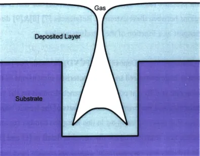
on the micro-meter scale. Figure 1 shows a sketch of an underlying substrate that has a

layer of material grown over it using CVD. In a typical integrated-circuit application the

dimensions of these features would be in the micrometer scale and the trench would be

created by photolithography or other similar etching processes. The deposited layer is

usually required to be very uniform and free of voids and cracks (as much as possible).

As such, much effort is expended into optimizing the manufacturing process to ensure

that the resulting profiles are acceptable with minimum use of time and materials.

Gas

flepoelted Layer

Figure 1: Illustration of layer growth over a substrate using chemical vapor deposition. Note the uneven thickness of the growth depending on the location along the trench.

The ability to accurately predict the shape of the deposited profile based on the process parameters is a very important factor in reducing CVD costs by reducing the guess-work

associated with efficiently producing acceptable quality features that are free of voids or other non-uniformities. Other applications that need accurate CVD models include the extraction of reaction parameters of active species. In such applications measurements of deposition profiles are compared with profile predictions to extract values for reaction probabilities and other related properties.

1.2 Previous Work and Background

References [5] [6] [15] give a good overview of the CVD process and the manner in which accurate modeling of transport within the feature affects the ability to produce integrated circuits with acceptable properties and cost. The ratio of the mean free path of the gas above the trench being studied to the characteristic length of the feature is the single most important factor in determining which model to use in describing the growth of the deposition layer. This ratio is known as the Knudsen Number (Kn) and varies inversely with the overall pressure of the gas above the trench. The transport of the deposition molecules to the substrate varies from being collision dominated at high pressures (Kn<<1) to being exclusively determined by geometric factors and boundary conditions at lower pressure (Kn>>1). A more complex behavior that is hard to predict appears in the regions between these extremes. References [7] [8]&[9] discuss the physics of gas transport as a function of the Knudsen number.

In Low Pressure Chemical Vapor Deposition (LPCVD) the mean free path between gas molecule collisions is large compared to the characteristic dimensions of trench and as a result the deposition rate at different points in the trench depends on the velocity

distribution of molecules and the manner different parts of the trench "shadow" each other. The equations that describe transport in this Knudsen number regime are similar to ones used in radiation heat transfer and are discussed in detail in [1] and [13]. LPCVD is commonly used in industry and very powerful deposition models have been successfully applied to many applications including 2D and 3D features as well as complex gas-surface chemical reaction models.

In Atmospheric Pressure Chemical Vapor Deposition (APCVD) the mean free path is very small compared to trench dimensions and the gas transport is determined by the standard Navier-Stokes flow model and the continuum diffusion model. Standard

methods for solving these equations are well known and have been applied to the solution of feature-scale transport modeling for many types of physical problems and gas-surface chemistries [l1],[10] and [16].

In this work we are interested in CVD problems that lie between the two aforementioned cases and have Knudsen numbers that are finite and gas transport is only properly described using the Boltzmann Equation. The Boltzmann Equation is a high-dimensional integral-differential equation that can only be solved exactly in a very limited set of special cases. There have been a number of attempts to numerically solve the Boltzmann equation that fall into two broad categories. The first category of methods try to make

significant simplifications to the physical processes by making broad assumptions that allow a quick solution of the transport problem. The most notable work in this class is the

Simplified Monte Carlo (SMC) technique by Akiyama and co-workers [2] which shows results that seem to be very promising. Unfortunately, this approach and others like it are always limited by the simplifying assumptions that they make and give quite erroneous results when the former are not satisfied. The other category of methods try to solve the full transport model making no simplifying assumptions usually using the Direct Simulation Monte Carlo (DSMC) method ([4] [3] and [12]). DSMC is the fastest

currently available method for solving the Boltzmann Equation. It was recently shown to provide accurate solutions of the Boltzmann Equation in the limit of infinitesimal

discretization [14]. Unfortunately previous attempts to use DSMC to model the CVD problem have not always given consistent results and suffered from fairly crude surface and chemistry models. In this work we develop a reliable CVD profile growth model based on the DSMC incorporating sophisticated chemistry and surface movement models.

1.3 Thesis Overview

The presentation of our work will be done in tree major parts. In Chapter 2 we describe our methodology for simulating feature scale surface evolution and present the details of the DSMC gas transport model used in our method. We will also detail the method through which we incorporate non-linear chemistry models into DSMC. In Chapter 3 we

give a number of examples that verify our methodology by comparing our results against exact solutions and other numerical methods in various flow regimes. In addition, we will present a number of trends that show the behavior of our model over a number of

important deposition parameters and compare the trends with previous results. Chapter 4 will be primarily devoted to a detailed discussion of the models used to simulate the

surface evolution with a particular emphasis on the Level Set Method. The fifth and last chapter gives a summary of our work and presents possible extensions.

References:

1. Cale, TS, Merchant, TP, Borucki, LJ, Labun, AH; Topography Simulationfor The

Virtual Wafer Fab. Thin Solid Films v. 365 152-175 2000.

2. Akiyama, Y, Matsumura, S, and Imaishi, N; Shape of Film Grown on Microsize

Trenches and Holes by Chemical Vapor Deposition: 3-Dimensional Monte Carlo

Simulation. J. App. Phys. V. 34 No. 11 1 1995.

3. Coronell DG; Simulation and Analysis of Rarefied Gas Flows in Chemical Vapor

Deposition Processes. PhD Dissertation MIT 1993.

4. Cooke, MJ and Harris, G; Monte Carlo Simulation of Thin-Film deposition in a

Rectangular Groove. J. Vac. Sci. Technol. A V. 7 No. 6. Nov/Dec 1989. 5. Bunshah RF (Editor); Handbook of Thin Film Deposition (Chapter5: Feature

Scale Modeling Vivek Singh). 2nd Ed., 2002.

6. http://www.batnet.com/enigmatics/semiconductor-processing/CVDFundamental

s/FundamentalsofCVD.html

7. Bird, GA; Molecular Gas Dynamics and the Direct Simulation of Gas Flows.

Oxford University Press 1998.

8. Vincenti, W and Kruger C; Introduction to Physical Gas Dynamics. John Wiley

and Sons, Inc. 1965.

9. Hirschfelder, JO, Curtiss, CF, Bird, RB; Molecular Theory of Gases and Liquids.

John Wiley & Sons, Inc. 1964.

10. Liao, H and Cale, T; Low-Knudsen-Number Transport and Deposition. J. Vac.

Sci. Technol. A V. 12 No. 4, July/Aug 1994.

11. Pyka, W, Fleischmann, P, Haindl, B, Selberherr, S; Three-Dimensional

Simulation of HPCVD-Linking Continuum Transport and Reaction Kinetics with

Topography Simulation. IEEE Trans. On Computer-aided Dsg. of IC and Sys. V.

18 No. 12 1999.

12. Ikegawa, M and Kobayashi, J; Development of a Rarefied Gas Flow Simulator

Using the Direct-Simulation Monte Carlo Method. JSME International Journal

13. IslamRaja, M, Cappelli, M, McVittie, J, Saraswat, K; A 3-dimensional Modelfor

Low-Pressure Chemical Vapor Deposition Step Coverage in Trenches and

Circular Vias. Appl. Phys. V. No. 11 70 1 December 1991.

14. Wagner, W; A Convergence Prooffor Bird Direct Simulation Monte Carlo

Methodfor the Boltzmann Equation. Journal of Statistical Physics V. 66 No. 3-4

1011-1044 Feb 1992.

15. Pricnciples of CVD. Dobkin DM and Zuraw MK. Kluwer Academic Publishers,

Dordrecht. April 2003.

16. Thiart, J and Hlavacek, V; Numerical Solution ofFree-Boundary Problems:

Calculations of Interface Evolution During CVD Growth. Journal of Comp. Phys.

CHAPTER

2:

METHODOLOGY

The goal of this chapter is to present our methodology for simulating chemical vapor

deposition in small scale trenches using the DSMC. This chapter will start with an

overview of the methodology outlining the major steps in the simulation process along

with how they fit with each other. The rest of this chapter will be dedicated to explaining

the details of two key parts of our methodology, namely, the DSMC model we are using

for gas transport and the non-linear chemistry model for surface interaction. The other

major part of the methodology, namely the surface evolution model, along with detailed

examples, will be presented in Chapter 4.

2.1 Methodology Overview

The basic approach we take here is to develop separate models for the gas transport using

DSMC and use the resulting deposition information in a separate surface evolution

model. An important assumption we are making here is that the surface profile is

stationary in the time scale relevant for transport. Such an assumption has been used in

previous deposition models and has so far been shown to be valid in many applications

[7]. In our methodology the simulation domain is terminated by boundary conditions

imposed by the large reaction vessel which provides a fresh stream of reactants. There

have been many attempts at creating integrated reactor/trench-scale models that directly

couple the deposition simulation to the reactor volume [6][8][13] though in many cases

such models are not necessary and are beyond the scope of this work.

(3) Boundary Movement Model

FA-dvenanceindary 1 mmip RefinelCoarsen Segnent Representation of Boundary

No

Yes

A

Refine Solution Parameters (Usually S and/or maxLength)

nal Profile Converg No

End No

----S-ele initial Parameters

(1)Create Initial Profile Segments I

I- - -- --

---(2)Find Deposition Rate using DSMC1

& ConNo

Yes

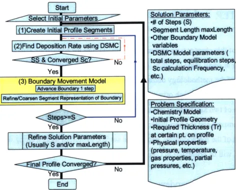
Figure 1: Block diagrams of procedure used in simulating CVD using DSMC with a non-linear chemistry model.

Figure 1 shows a flow diagram of our methodology for calculating the profile resulting from CVD after a finite amount of time tfinal using S steps. We start by selecting an initial set of parameters that control how refined our profile and DSMC models are. The

selection of the proper parameters to give converged results requires some experience and in general the calculation will be repeated with more detailed parameters to ensure the final profile is converged. An initial profile is created based on the problem specifications (Step 1 in Figure 1), which is used as an initial step of our DMSC calculation. The

DSMC calculation (Step 2) is run long enough to ensure converged results are reached by

meeting two important requirements. The first is that the steady state is reached as judged

by the change of the total deposition rate over time. The other requirement is that the

chemistry model -if one is used- is converged as will be explained in section 3. The resulting deposition rate is then used by the surface model (Step 3) to create the surface resulting after time= tfinal /S. The boundary model includes provisions for ensuring the properties of the resulting surface fit within the solution parameters specified at the start (for example the length of all segments<maxLength and so on). These steps are repeated

Solution Parameters:

4# of Steps (S)

-Segment Length maxLength

-Other Boundary Model variables

-DSMC Model parameters ( total steps, equilibration steps

Sc calculation Frequency, etc.)

Problem Specification: 'Chemistry Model 'Initial Profile Geometry 'Required Thickness (Tr) at certain pt. on profile

-Physical properties (pressure, temperature, gas properties, partial pressures, etc.)

S number of times until the surface profile at end of time tfinal is found. The whole process

can be repeated with more refined parameters to confirm the convergence of the final

deposition profile.

2.2 DSMC Gas Transport and Deposition Model

As mentioned before, the Direct Simulation Monte Carlo method is used in this work to

account for the gas transport in our CVD trench model. DSMC was invented by Bird [1]

in the 1960's as a method of numerically solving the Boltzmann Equation for a wide

variety of conditions. The DSMC method is fairly well documented (See

[1],[9],[l0],[1l],[12]&[13]) and so the next sections will only discuss aspects of our

implementation that are special or non-standard.

Although the particle dynamics in DSMC are three dimensional, this thesis considers

infinite trenches for which a two-dimensional model is sufficient. Nothing fundamentally

limits the applicability of our work to 2D problems, although in 3D there may be some

complications with our boundary movement model and of course

,

the computation cost

will increase. In Chapter

5

we discuss to possible ways for extending our methodology to

handle these cases.

X=0 Plane

Symmetry BC

z

x

Segments Defining Trench Profile

x

aWith

Sticking Coefficient

Symmetry BC 4x 10 ax 10~ 6x 10-6x 10 4x 10-8x 10 2x 10

Figure 2: Plot showing the segments of a deposition profile and two different boundary conditions of the DSMC domain. A cyclic (periodic) boundary condition is also applied in the Z-Direction to simulate the effect of an infinite trench.

Figure 2 shows a sketch of the domain and boundaries of a typical DSMC run used in our methodology. The domain is divided into a uniform 2D array of square cells of side lengths of / the mean free path (k). The trench segments are free to move in the domain

across any of the cells and to ensure that the cell collisions are processed properly, the volume of all cells is calculated using a simple Monte Carlo integration technique at the start of every DSMC step. The domain height in the z-direction is also set to roughly /3 X

and a cyclic boundary condition is applied in that direction to simulate an infinitely long trench. The length of the cell along the z-direction is not important because this is fundamentally a 2D problem and in fact we could have totally ignored the positions and movement along this axis to save on computational resources with no effect on the results. Finally, our implementation is set up so that the gas particles in the domain can be divided into an arbitrary number of species that can be independently tracked at all times.

The gas enters the simulation domain through the open wall boundary condition that is applied at the x=O plane. Particles that cross this boundary and leave the domain of interest are deleted. This boundary condition essentially matches the simulation to an

infinite reservoir (x<O) of specified number density, composition and overall average velocity. Incoming particles are created by filling a larger region (between 0 and -4 X) with particles with random initial positions and a Maxwell-Boltzmann velocity

distribution every time step. The movement of these particles is tracked and the ones that drift into the DSMC domain are kept while retaining their velocity and new position. Although this is more complex than simply creating the particles at x=0 with a biased Boltzmann velocity distribution, it is done to ensure that the particles created not only have the correct distributions for position and velocity but also maintain the correct

correlation between these two variables.

The other set of boundaries are created by the trench (shown in red in Figure 2) and the symmetry segments at the ends of the domain (shown in blue). Gas particles in the domain are moved using the standard advection schemes used in DSMC. Collisions with the domain boundaries are also similar in spirit although the arbitrary deposition shape requires the discretization of the latter in a larger number as small linear segments. As the number of boundary segments grows large (in a typical trench there are 50-200 segments) the computational cost of the particle advection step is increased by the same degree. This can have a very significant effect on the speed of our transport model, particularly when we have a large number of segments and/or a low Knudsen number. As will be explained in Chapter 4, there is a simple optimization that can be made to dramatically improve the speed while making no compromises in particle movement accuracy.

Symmetry boundary conditions can be simply applied by specularly reflecting gas particles that collide with the symmetry boundaries. In contrast, the treatment of particles that collide with the growth surface involves the absorption of particles with a certain predefmed probability (called the Sticking Coefficient); the remainder are diffusely reflected back into the domain. In our calculations both the reactor and the trench are held at the same temperature though it is easy to have different temperature distributions or even non-Maxwell-Boltzmann velocity distributions inside the reactor domain (x<0).

are defined as statistical averages over small regions of space. In addition, statistics are collected for the number of particles that hit each growth surface segment and the number of particles that "stick" to a segment. These are later used to infer the partial pressure of each species as well as the deposition rate at each segment.

2.3 Deposition Surface Chemistry Models

The emphasis in this work is to study CVD in features due to chemistry that is dominated

by gas-surface interaction. There are methods to incorporate gas-gas chemistry in DSMC

models ([1] and [2] for example) though it seems that their effect is not always important

in feature transport models

[5].

More details will follow in Chapter 3 but as a general

trend lower sticking coefficients (i.e. particles needing more collisions with the wall before they stick to it) result in better quality profiles while higher sticking coefficients cause the formation of voids and cracks. Traditionally, the sticking coefficient is taken to be a constant that does not change along the trench length or as the trench changes shape

due to deposition. Usually "curve fitting" is used to match a constant sticking coefficient

with the profiles measured from experimental SEMs and despite its crudeness this method is very successful in producing good estimates of sticking coefficients for many

conditions [3].

A number of successful attempts have been made to incorporate more sophisticated models for the calculation of the surface sticking coefficients in both CVD [5] and physical vapor deposition [6]. Our method for calculating Sticking coefficients based on chemistry models for CVD is similar to the method available in the literature though it has been modified to be used within our DSMC framework.

To understand how the sticking coefficient is calculated, assume that there are two gases

in our domain that react according to the following formula:

A+ B -+

y

C(s) + 6 D ₍₁₎

$

is the number of moles of species B that react with each mole of species A. and likewise,

y is the number of moles of species C deposited for each mole of species A that reacts.

6 is the number of moles of species D returning into the gas from the surface for each mole of species A that reacts.

Furthermore, assume that an analytical formula is available for the reaction rate of reaction 1:

Rate=RateA =T,PPA,PPB,PPD,---] (2)

where ppj is the partial pressure of species

j.

We proceed by "splitting" the reaction equation into two equations that involve only one of the reactants, for example:

A - 1/2y C(s) +/26 D (1 a)

and B -+ y/ C(s) +% 2 /D (lb)

The partial pressures used in (2) can be inferred from the average number of particles that intersect each segment by the following method [4]. We first try to find the number density starting from the analytical formula for the flux of particles from a gas at equilibrium:

n 4 Flux

Flux=-C == n=

4

We then proceed to use the ideal gas law to relate the flux of incoming particles to the partial pressure of an equilibrium gas:

Flux

pp= rnRT ==pp =4 mRT

We finally calculate the particle flux into a segment by dividing the effective number of particles that hit the segment by the length of the run and the area of the segment. The implied partial pressure is then used in (2) to find the local rate of reaction at the segment. With the reaction rate at hand the sticking coefficient of species

j

and for segment i can be calculated from the reaction rate' of the species at that segment as follows:

Scoj,i)=Ratej (i)/Fluxj(i) (4)

Moreover, the number of moles of species C that is deposited is tracked by adding y /2 to its counter each time species A is absorbed and /2 y/P each time species B is absorbed.

It is important to realize that the way the reaction equation (1) is split to (la) and (lb) is generally not important as long as the correct ratios for sticking coefficients and reaction rates are recovered in the limit of large number of reacting molecules colliding with the surface. The rationale is that equation (1) is a simplification that only agrees with the real reaction mechanism in an average sense and does not include the details of the real reaction. In a similar manner, it is important that DSMC reproduces the gross chemical behavior in an average sense and not necessarily during every collision.

There are two ways of calculating the deposition flux rate at each section. The first is to directly record the total number of particles absorbed on each segment and convert that to a deposition flux rate. The second method is to use the reaction rate form (2) to calculate the deposition rate at each point (in this example Deposition Rate =RateA*y). Although these two methods are equivalent in principle, the results of the later are much less noisy when a significant number of particles that hit the wall do not react with it.

The final issue that has to be addressed is the creation of byproduct species that can be important in finite Knudsen numbers. The byproduct species is created after every collision according to its molar ratio to the reacting species in the split chemical formula. For example, in Reaction (la) /26 particles of species D are created every time species A is adsorbed and likewise /2 6/ particles of D are created each time Species B reacts with

' Actually the reaction that should be used is Min[Rate, FluxA, FluxB] to ensure that the depletion of one species limits the rate of the total reaction.

a segment. The new species are introduced in the domain at the point that the reacting

particle hits the surface and they are moved for the balance of the time step duration after

the original particle reached the segment. One complicating issue arises when the number

of byproduct particles to be created is not an integer and can be dealt with in one of two

ways. One way is to split the original reaction equation such that an integer number of

byproduct particle has to be created every time a reaction happens. The other solution

that is more general is to create an extra particle with a probability equal to the fractional

part of the number of particles.

Finally, there have been a number of bold assumptions made in our approach in

calculating the sticking coefficients that are not guaranteed to hold in all cases. The most

notable example of this is the assumption of an equilibrium gas distribution that results in

(3) that we use above. In spite of this, the method is able to give correct results in many

different cases and in particular it has been verified at high Knudsen numbers

[5][7]

where gas particles are sometimes very far off from the equilibrium velocity distribution.

This is probably because the reaction rate (2) is much more a function of the number of

molecules that arrive at the surface and their average temperature and not a strong

function of the velocity distribution function of these molecules.

References:

1. Bird, GA; Molecular Gas Dynamics and the Direct Simulation of Gas Flows. Oxford University Press 1998.

2. Boyd, I, Bose, D and Candler, G; Monte Carlo Modeling of Nitric Oxide

Formation Based on Quasi-classical Trajectory Calculations. Phys. Fluids V. 9

No. 4 1162-1170 April 1997.

3. Junling, L; Topography Simulation of Intermetal Dielectric Deposition and

Interconnection metal deposition Process. PhD Dissertation Stanford University

March 1996.

4. Cale, T, Gandy, T and Raupp G; A Fundamental Feature Scale Modelfor Low

Pressure Deposition Process. J. Vac. Sci. Technol.A V.9 No.3 524 1991.

5. Cale, T, Richards, D and Tang, D; Opportunities for Materials Modeling in

Microelectronics: Programmed Rate Chemical Vapor Deposition. Journal of

Computer-Aided Materials Design, V. 6 283-309 1999.

6. Rodgers, S; Multiscale Modeling of Chemical Vapor Deposition and Plasma

Etching, PhD Dissertation MIT February 2000.

7. Cale T and Mahadev V.; Low Pressure Deposition Processes. Thin Films V. 22

172-271 1996.

8. Coronell DG; Simulation and Analysis of Rarefied Gas Flows in Chemical Vapor

Deposition Processes. PhD Dissertation MIT 1993.

9. Alexander, F and Garcia, A; The Direct Simulation Monte Carlo. Comp. In Phys.

V.11 No. 6 588-593 1997.

10. Garcia, AL; Numerical Methodsfor Physics (2nd Ed.). Prentice Hall 2000.

11. Bird, GA; Recent Advances and Current Challengesfor DSMC. Computers Math.

Applic. V. 35 No. 1/2 1-14 1998.

12. Oran, E, Oh, C, Cybyk, B; Direct Simulation Monte Carlo: Recent Advances and

Applications. Annu Ref Fluid Mech. V.3 403-41 1998.

13. Hudson, Mary, Bartel, Timothy; Direct Simulation Monte Carlo Computation of

Reactor-Feature Scale Flows. J. Vac. Sci. Technol., A, V. 15 No. 3,1 559-563

CHAPTER

3:

VERIFICATION

The goal of this chapter is to demonstrate that our CVD modeling methodology is in agreement with already existing results that are exact, published or experimentally verified. We will start by describing a number of important definitions that will be useful when analyzing results presented in this and other chapters. The results will be grouped and presented in three different sections based on the Knudsen number and the surface chemistry model. The first section will discuss results of depositions at very low pressures (Kn--oo) and with a constant surface sticking coefficient. The second section will describe deposition results which are in the same Knudsen regime but with a non-linear chemistry model which predicts the surface sticking coefficients. We will finally turn our attention to verification problems at high pressure (Kn->O) by comparing our results with results from a continuum diffusion model. In addition, trends of key parameters will be presented in an attempt to give a feel for the effect of varying the Knudsen number.

3.1 Definitions of Key Terms

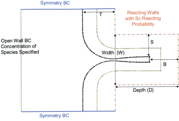
Clear definitions of key ideas and terms are needed before proceeding to present the results. The definitions of the terms used here are similar to the ones used in the literature (see for example [10]) with only some minor modifications or variations. Figure 1 shows a sketch of a typical deposition problem along with dimensions of key importance.

Symmetry BC T Reacting Walls with Sc Reacting Probability Open WalI BC Concentr tion of - .... ...

Species $pecified Width (W)

...'rn uu..

Depth (D)

Symmetry BC

Figure 1: Sketch of basic trench showing important dimensions used to define commonly used terminology.

The Aspect Ratio (AR) is the ratio of the width of the trench (W) to the Depth (D) for the

deposition profile in the initial state. As the CVD proceeds, different parts of the profile advance at different rates and the emerging profile is described by a number of different measures. The Corner Step Coverage (CSC) is the ratio of the side length of the thinnest part in the bottom of the trench (S) to the thickness at the top (T). The Bottom Step

Coverage (or simply the Step Coverage) is the ratio of the middle of the bottom of the

trench (B) to the top thickness T. The Flux Step Coverage (FSC) is the step coverage calculated based on the deposition rate at the initial geometry. Deposited profiles that have high step coverages (called Conformal profiles) are desirable since they result in profiles that do not develop voids when the deposition is continued until the mouth of the feature is closed.

3.2 Low Pressure Deposition with Constant Sticking Coefficient

(Kn-+oo)

In this section we start by comparing the accuracy of our code with relation to an exact

analytical solution. We then proceed to compare our deposition maps and resulting trench

profiles to results from specialized low pressure (Kn-.oo) deposition codes that have been

independently verified. Next we proceed to compare our new DSMC results to previous

attempts at modeling trench deposition for arbitrary Knudsen numbers. As we will see we

are generally able to reproduce published results at high Knudsen numbers but have

found that we disagree with some of the results for published arbitrary Knudsen numbers.

3.2.1 Comparing LPCVD Results to Analytical Limits and Specialized Programs

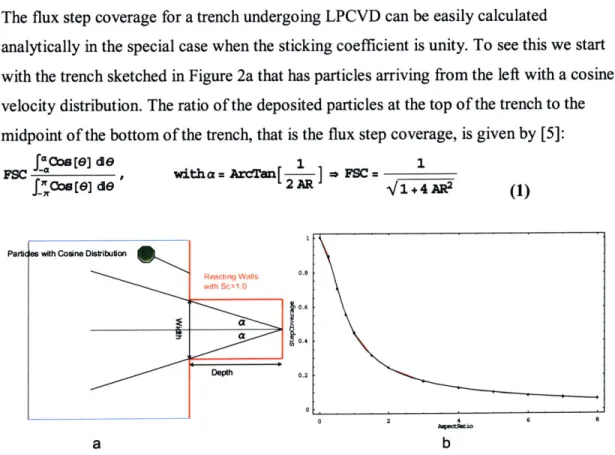
The flux step coverage for a trench undergoing LPCVD can be easily calculated

analytically in the special case when the sticking coefficient is unity. To see this we start

with the trench sketched in Figure 2a that has particles arriving from the left with a cosine

velocity distribution. The ratio of the deposited particles at the top of the trench to the

midpoint of the bottom of the trench, that is the flux step coverage, is given by

[5]:

Ja cos[eJ

de [1 1 FS .

FSC - [ , with a= ArcTan ___FC=

",Cos[e] de 2 AR 1,+ 4A

(1)

Partic es with Cosine Distribution

Reactn Walls 0.8

Dwith 021.

a b

Figure 1: (a) Sketch of trench with a sticking coefficient=l. All particles that come from the left are absorbed at the surface. (b) A plot of the step coverage for different aspect ratios. Points are DSMC results while the solid line is the prediction of the analytical formula.

Figure 2b shows a plot of the analytical formula along with the DSMC results for

trenches with aspect ratios ranging from 0 to 8. Clearly there is excellent agreement

between the DSMC and analytical results with differences only due to statistical noise.

Unfortunately, the above simple analytical model cannot be extended to cases with Sc<1

or for geometries that are more complex than a simple trench. The problem of solving for

the transport at the radiation limit is however very well understood and much advanced

work has been done in this field [3][2]. One implementation of this work that has been

extensively tested in simple and complex cases is a profile simulator known as EVOLVE

developed by Cale and co-workers[7].

Figure 3 shows a sketch of a moderately complex trench (in red) with particles coming in

from the left with a cosine (equilibrium) velocity distribution. The results for the

deposition profile along the trench length are plotted for both EVOLVE (3b) and DSMC

(3b) for two separate sticking coefficients. The agreement between the two codes is

almost perfect implying that our particle tracking methods in complex geometries are

indeed accurate.

Rellect e W alis - 1 F-SF-1O0 1 McI. ofSPI L L F-05--- 0.8 .0. * Sc0.5 D9 06 0. R-cting A-3 Opei to reservoir 0. Species 1 ccns.0.5 Species 2 cons.=0.5 B-3 C= 02 / 0 0to0uI,0 0-2 04 0.6 0.8 1 20 40 60 80 100 normed arciengr

a

b

C

Figure 3: (a) Sketch of complex trench. (b) EVOLVE result for both 1.0 and 0.5 sticking coefficient. (c) DSMC results for the same sticking coefficients.

We now proceed to look at an even more complex example with multiple species and an asymmetric trench (Figure 4). In this example we have low pressure gas with 3 species each with a unique initial flux rate and sticking coefficient at the surface. Species 1 and 2

come in at similar proportions from the left while species 3 is only created as a byproduct

of the deposition of Species 1 at the wall as follows:

Spi

-+

3 Sp3

+

Deposition

@

wall (Sc[Spl]=0.5)

Sp2 Does not react

Sp3 -- no byproduct + Deposition @ wall (Sc[Sp3]=1.O)

As can be clearly seen from Figure 4 the agreement between DSMC and EVOLVE is

exceptionally good for all species. It is interesting to note how there is no deposition of

Species 3 in the trench areas facing the left since no particles of that species come in from

the boundary on the left and there are no gas-gas collisions to return particles back to the

surface.

Sp1-.Sp3 1.2

- Sp2 doesn't react -- Reaction rate of SP3

1 - Reaction rate of SP1 1 0.8 0.8 Sp 0 Cl) 06 0.6

0

Asymmetric Tren 0.4 0.4 __ _ _ _ __ __ _ _ 002 0.2 0.2 02 0.4 0.6 0.8

Figure 4: Complex profile, EVOLVE Result and DSMC Result Respectively. The normalization is using the deposition rate of Spi on the part of the trench facing left.

Our next example compares results for actual deposition profile evolution based on the flux data from DSMC. Chapter 4 gives more details on how we model and incorporate deposition rate data into profile evolution. The example is of a trench of unity aspect ratio and a constant sticking coefficient of 0.35. Figure 5 shows the result of our calculation (light color) along with published results calculated by SPEEDIE (an other LPCVD deposition software) [2]. The agreement is very reasonable particularly since the Simple Node Tracking method was used with only 20 calls to the DSMC program. Chapter 4

contains an other LPCVD example with a constant sticking coefficient in which DSMC

results are compared to EVOLVE profiles.

0 SPEEDIE

* DSMC Calculation

- mlI

Figure5: Deposition profile results for trench with aspect ratio=1.25 and a sticking coefficient=0.35. Dark lines are for SPEEDIE while light ones are for our DSMC methodology using a simple node tracking surface model.

3.2.2 Step Coverage Trends Calculated for Low Pressure Deposition with

Constant Sticking Coefficients

Now that we have established the reliability of our approach in predicting the deposition

profiles, we will present a few plots that summarize the profile behavior at different

sticking coefficients. Furthermore, we compare our results with those obtained with

various other CVD methods designed for the transition regime

(-

0.05<Kn<10). The first

plot (Figure 6) is of the corner step coverage in a unity aspect ratio trench as a function of

the sticking coefficient. The step coverage is calculated at the point when the thickness of

the deposition layer is half the width of the feature and in all cases the profile is

the results published in [4] of the same set of cases calculated using a different

DSMC-based method. The agreement between the two trends is very reasonable and the

difference is probably mainly due to the variations of profile moving model.

Comparison Between (4] & DSMC Corner Step Coverage 0.7 0.6 En, 0.5 rt $ Curve From 4 0.4 DSMC 'S0 .3 0.2 0.1 0.2 0.4 0.6 0.8 Sticking Coefficient

Figure 6: Step coverage versus sticking coefficients of trenches with AR=1 at a deposition

thickness=%A width of feature and Kn=oo. Plot compares our DSMC results with those published in 141.

A different parameter (the bottom step coverage) is plotted in Figure 7 for the same set of

cases. Again the two red and blue curves are for the step coverages calculated at a

thickness of /

2

*width of the initial trench similar to Figure 6. Upon examination it is clear

that the results in [4] do not agree with our calculations even when the solution

parameters are varied.

Comparison Between Different Methods of Calculating Bottom Step Coverage 0.9 _________ Bottom S/C From [4] 0.8 ... ___ DSMC 0 0.7 0.6 0.9

Upper Analytical Limit

0.2 0.4 0.6 08

Sticking Coefficient

Figure 7: Results for step coverage versus the sticking coefficient for a AR=1 trench at Kn=oo. The red curve is result reported in 141 while blue curve is our DSMC calculation. In both cases the step coverage is calculated at a deposition thickness='%trench width. The analytical result is from equation (1).

A number of clues need to be considered to confirm that our results are indeed the more

accurate ones. To begin with, our results agree well with other codes that have been

designed and verified in the vacuum limit (namely, EVOLVE [7] and SPEEDIE [2][18]).

Also, equation 1 gives us a strict upper limit on the step coverage when the sticking

coefficient is 1 because the step coverage decreases with time. The red curve clearly

violates this inequality. Finally, the lack of detailed experimental results verifying the

trends of [4] also reduces confidence in their accuracy.

3.3

Surface Step Coverage for LPCVD using a Non-Linear Chemistry

Model

This section presents our results for the simulation of LPCVD on 2D trenches with a

non-linear surface chemistry model and comparing them with published results. Our goal is to

verify our methodology and code by reproducing Kn-+oo results where the particle

velocity distribution is the furthest away from equilibrium and it is where we expect the

greatest deviation if our method does not hold. In what follows we will proceed to

explain the chemistry model that will be used in the examples of this section followed by

a detailed discussion of our results for a trench on an aspect ratio of 10. We also discuss

the convergence of the step coverage. We will then show that our methodology

accurately reproduces EVOLVE trends over a wide range of model parameters.

3.3.1 Tungsten Deposition Surface Chemistry Model

We selected the reduction of Tungsten from tungsten hexafluoride as the non-linear gas

surface chemical reaction to model in this section. Nothing in our algorithm or

implementation is unique to Tungsten and only a change of the chemical species and the

reaction rate equation is needed to be able to model other reactions (see [10], [7], [3] or

[11] for details of modeling other reactions). Reference [16] gives a detailed discussion of

modeling Tungsten chemistry but for this example we will use the simple formula[ 17]:

WF6+3H2-+W (s) +6HF (1)

and the reaction rate:

-8800 P6 1 + KF

Rate= 7.16233Expl T

]

1H 2 " 1+KFPP6

(a)

T pp6 1+K

5996(g

where:

Rate: is reaction rate/mole of reactants [mol/(s*m

2

)]

T: Temperature [K]

PH2 : Partial Pressure of H2 [Pascal]

wF6: Partial Pressure of WF₆ [Pascal]

PPF6: Partial Pressure of WF₆ at entry [Pascal] KF: Constant=7.5/Pascal

As explained in Chapter 2 in our model the reaction is actually split up into two reactions that on average reproduce (1) as follows:

1 WF6 1 W(s) +3HF 2 (2) and 1 H2-- W (s) +HF 6 (3)

with a H2 deposition rate equal to the times the rate defined in (la).

In our calculation we ignore the creation and the transport of HF. This saves on

computing resources and does not affect the results because at high Kn values the lack of collisions means that the increase in HF number density does not reduce the flow of the other species to and from the surface.

3.3.2 Detailed Example of Tungsten LPCVD

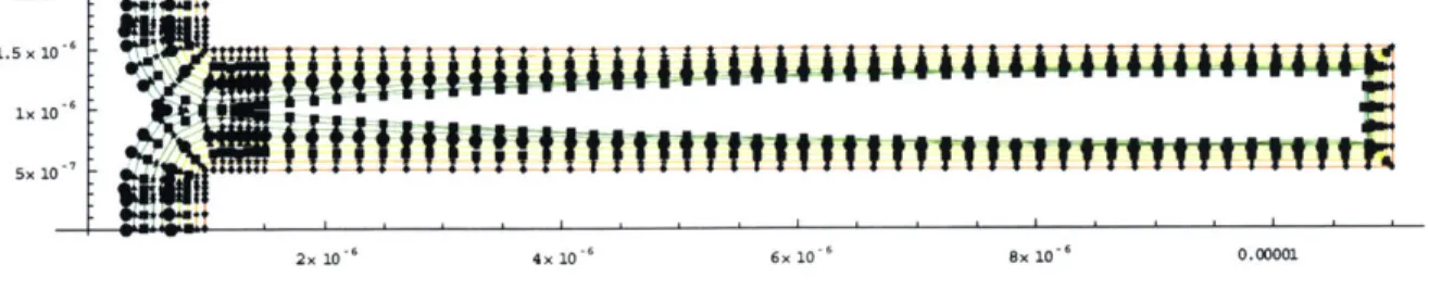
The first example of Tungsten deposition will be in a trench with an aspect ratio of 10. The simulation is carried out by taking H2 with an incoming partial pressure of 4.66

Pascal and WF6 with a partial pressure of 0.466 Pascal. The surface profile is integrated

until a cavity is created when the feature pinches off as can be seen in Figure 8. The simple node tracking model was used to follow the evolution of the profile shape and the step coverage value at closure is predicted within 1% of the published value. The

integration of the profile was carried out with only 8 DSMC program calls from start to closure.

2x 10

-1.5 x 10 6

ix 10

5x 10 7

2x 10 4x 10' 6x 106 8x 10-' 0.00001

Figure 8: Plot of deposition profile of an AR=10 trench up to closure.

Figure 9 shows a plot of a number of important parameters along the length of the profile

for both species as the feature is filled. As the feature fills the partial pressure of WF

6

significantly decreases inside the feature which results in a drop

in

the deposition rate.

Since the partial pressure of H

2

is not significantly reduced, the lower deposition rate

results in a lower H

2

sticking coefficient in contrast with the sticking coefficient of WF

6

which increases to a maximum value because la is essentially linear at lower WF

6

S/C(E.) 0.08 0.07 0 .06 . 0.05 i k 0.04 * 0.03 1~ pl'04 0.6 .8i Dp Rite (_%a) 4x 10 3x 10 2x 101 0x 100 0.2 0.4 0.6 0.8 1 0.4 0.3 0.2 0.1 0.2 0.4 0.6 0.8 1 4aq -q Saq . tq Stq Stq SStg U tg - -q Nxb . . 1 2 3 4 5 6 7 8 9 10 1 2 3 4 5 6 7 8 9 10 1 2 3 4 5 6 7 8 9 10 SfC()3 0 042 0.00M4 0.2 0.4 0.6 0.8 1

Dep Paite ( O2)

1.4 x 102 1.2 x 10 2 ,X 1021 8x 10, 1 * \ * 6x10 4x 10 i 2x 10. . 0.2 0.4 0.6 0.8 1 1amt . Pem . ( 2) 4.65 4.625 4.6 4.575 4.53 4.525 0.2 0.4 0.6 0.8 1

Figure 9: Plot of key parameters versus trench length for the 10 steps that are shown in Figure 8. The left column is for Species 1 (WF6) and right column is for Species 2 (H2). Feature is closed after step 8.

Critical to the accuracy of the results presented above is the calculation of the sticking

coefficient in a robust manner. An approach that we have found to give reasonable

accuracy was to first perform an "equilibration" run with short intervals between Sc

re-calculations (details in Chapter 2). We then use the resulting sticking coefficient map as a

starting guess for a longer run to confirm convergence. The equilibration here is

numerical in nature since at such high Knudsen numbers the problem is almost

immediately steady state as far as the transport is concerned. The sticking coefficients are

k aq A- atq Gtq s tef * a4 Sster +St% 9,4 I- Eq 1 2 3 4 5 6 7 8 9 10 1 2 3 4 5 6 7 8 9 10 1 2 3 4 5 6 7 8 9 10

considered converged when there is no appreciable systematic drift in their values and the only change that happens with time is due to the reduction of noise because of better

sampling.

3.3.3 EVOLVE and DSMC Trends

To further validate our methodology, calculations similar to the one detailed in the last section are preformed and compared to results of EVOLVE in [10] and [17]. Figure 11 shows a plot of the corner step coverage at closure of a unity aspect ratio trench at a number of different temperatures with WF6 and H2 concentrations identical to those in

the last section. DSMC accurately reproduces the EVOLVE trend with the majority of the points only 2-3% away. Figure 12 is a plot of the step coverage at 723K of trenches of various aspect ratios for EVOLVE and our DSMC program. A similar agreement between the two programs can be seen and in fact the agreement on the AR 10 trench is within 0.5%! 80 60 40 20 .__..__..__. . 7kTp. (K) 700 750 800 850 900

Figure 11: Plot of step coverage vs. temperature for Tungsten CVD on an aspect ratio 1 trench with a

pp H2/ppWF6=10. The solid line is taken from 1101 while the points are DSMC results. Error bars

Step Coverage Vs. Aspect Ratio 100 80 0 M 60 LQ d 40 20 1 2 3 4 5 6 7 8 9 10 Aspect Ratio

Figure 12: Step coverage values for Tungsten CVD for various aspect ratios at a temperature of 723K and ppH2/ppWFe=10. The solid line is from 1101 while the points are DSMC results with ±5%

error bars.

3.4

CVD at High Pressures (Kn-+O)

3.4.1 Continuum and DSMC Model Results

Taken together, the results in the last section give us confidence in our methodology for

both simple and complex non-linear surface chemistry models in the very low pressure

(Kn-*oo) regime. In this section we present our DSMC results for high pressure CVD and

compare them with results obtained using continuum diffusion finite element analysis

(FEA) techniques using a constant sticking coefficient.

A constant sticking coefficient is used here to simplify the continuum equations and their

solution. Our DSMC methodology would be identical if we wanted to use a non-linear

surface chemistry model. The development of special boundary conditions for the

continuum model with a non-constant Sc on the walls is a bit more involved and is

beyond the scope of our work though it is discussed extensively in [8], [9] and [12]. In all

of our lower Kn number examples the particles that react with the wall release physically

identical but non-sticking particles that are released back into the gas. This is done to

ensure that there is no net mass flux into the surface, thus canceling convection terms

from the continuum model.

The equation that determines the steady state number density (ni) of species i is [13]:

E6. vn = 0

D. is the self diffusion coefficient of our gas and is available from standard gas dynamics

theory. For hard spheres its value is [14]:

3 V'rmkT

8 7Wdmn

where d is molecule diameter, n is the number density, m is mass and k is the Boltzmann

Constant.

-7~ 010r c 550 Symmetry BC 10 -Deosition 24 Pts S P1 Surface

J

16Pts 0 -- - - S y m m e try B C f 1 P ts o Point of Measurement 5W 0.5 0 0. 1 15 2 25 3:%5 0 05 I 15 2 25 3 X10- 1- 1~

Figure 13: Finite Element Model of the continuum diffusion problem solved to compare with the

DSMC calculation results.

Figure 13 shows the meshed solution domain used to solve the problem-for a trench with aspect ratio AR= . A symmetry boundary condition (dni/dy=O) is used to impose a no mass flux state on the top and bottom edges, while a constant number density nO is assumed along the left edge to represent the domain inlet. The exact value of the imposed

4.5 4 3.5 3 152.5 2 1 .5 1 0.5

number density is taken from the DSMC results to account for slip effects and is the only

input imported from that model. At the deposition surface the following boundary

condition is used:

1 d n

Nbss Flux at Tre.h Edges = 1Cn= D., dn

4 d mm-al

This physically means that at the deposition edge of the domain the particle flux from the

domain must be equal to the diffusive flux due to the number density gradient in the

domain.

The continuum domain is meshed and solved by using the Pdetool package of MATLAB

[15] and the solution is taken to be converged when its values at the deposition edges do

not change as the domain mesh is refined. The flux rate along the trench is calculated by

the flux formula from equilibrium gas dynamics:

1

-TrenhFlux = - C npsw.±icz

4

1' 10 (D 0 CD (D t.J 8' 4' 1026 1026 1026 10 20 30 Segment/node number

Figure 14: FEM and DSMC results for the deposition rate along the trench at the measurement points sketched in Figure 13. The error bars are ±5% of local value. Problem parameters: Sc=1.0

500,000 particles Kn=0.03 and AR=3.

mnlized De. Rate

1

0.1

0.01

0.001

0.

0001-ruNuized DeoSitim Rate alaig Iagth

0 2.5 5 7.5 10 12.5 15

Figure 15: Comparison between the deposition rates as calculated from DSMC and FEA along the length of an AR=3 the trench with a Sc=1.0. We are plotting the natural log of the solution because there is a large change in magnitude between the top and bottom of the trench. The values are

normalized to the deposition rate of the node at the top of the solution domain.

- Continuum DSMC 40 DSMC MATLAB Node # 17.5

Figures 14 and 15 plot the deposition rate of the problem as calculated by DSMC and the continuum problem explained in the last paragraphs. Both calculations were performed using a gas at 300 Kelvin and an appropriate pressure to give a Kn=0.03 on a trench of 1 pim width. For the DSMC calculation care was taken to ensure that steady state was reached before starting to take samples to measure the deposition rate. Figure 14 shows the deposition rates for a V aspect ratio trench with error bars ±5% of local value. Clearly, the agreement for both the deposition values along the trench and the inferred flux step coverage is excellent. The same calculations are made for an aspect ratio 3 trench of the same width and gas properties. Figure 15 shows a log linear plot of the deposition rate along the trench normalized to the rate at the axis of symmetry at top of this trench. Again the agreement is very good particularly when one notes the drastic change in the deposition rate value between the top and the bottom of the trench. These test problems, as well as other not presented here, indicate that our DSMC simulation captures gaseous transport for all ranges of Knudsen numbers.

3.4.2 Step Coverage Trends with different Knudsen Numbers

0.8 0.6 - -- *Km 0.4 -- R- I =10 0.2 0.2 0.4 0.6 0.8 1

Figure 16: Flux step coverage at base versus Kn and sticking coefficient for an aspect ratio 1 infinitely deep trench. Argon gas was used with a trench width of 1 pm.

A feel for the trends in this class of deposition problems can be gained by examining the plots in Figure 16. The flux step coverage is plotted against sticking coefficients for a number of different Kn values. This set of calculations was carried out using Argon on a unity aspect ratio trench with different pressures to vary Kn. As expected, the step coverage is unity when the sticking coefficient is zero and monotonically decreases with higher sticking coefficients for all values of Kn. There is also a significant decrease in the flux step coverage as the Knudsen number is decreased in all cases. This is in qualitative agreement with the results of Cooke and Harris [1] as well as Kobayashi et el. [4]. The decrease in step coverage is easily explained by the fact that collisions work to

"segregate" regions of trench and result in larger differences in number densities and flux rates. Although step coverage at high Kn values does not change with different gases and temperatures it is a function of these and other parameters at lower Knudsen numbers. This is because the diffusion coefficient and hence the transport is a strong function of these parameters which means that no simple universal trends can be created for lower Knudsen number problems.

We finally would like to note that when at low Kn it is important to include enough of the domain above the trench in the model. This is done to ensure there are no concentration gradients across the open wall boundary condition that would cause changes in the deposition rates as a function of area included in the model. In our work we found that a distance of about 1-2 trench widths gave sufficiently accurate results but it must be understood that this may vary significantly with different problem details and only experimentation with different lengths can ensure convergence. A discussion of this issue in the continuum case (where the issue is most significant) can be found in [9].

References:

1. Cooke, MJ and Harris, G; Monte Carlo Simulation of Thin-Film Deposition in a

rectangular Groove. J. Vac. Sci. Technol. A V.7 No.6. Nov/Dec 1989.

2. IslamRaja MM, Cappelli MA and others; A 3-Dimensional Modelfor Low

Pressure Chemical- Vapor-Deposition Step Coverage in Trenches and Circular

Vias. J. Appl. Phys. V. 70 No. 11 1 December 1991.

3. Cale, T, Richards, D and Tang, D; Opportunitiesfor Materials Modeling in

Microelectronics: Programmed Rate Chemical Vapor Deposition. Journal of

Computer-Aided Materials Design, V. 6 283-309 1999.

4. Ikegawa, M, Kobayashi, J, Maruko, M; Study on the Deposition Profile

Characteristics in the Micron-scale Trench Using Direct Simulation Monte Carlo

Method. Transaction of the ASME Fluids Engineering Division V. 120, June

1998.

5. Akiyama, Y, Matsumura, S and Imaishi, N; Shape ofFilm Grown on Microsize Trenches and Holes by Chemical Vapor Deposition: 3-Dimensional Monte Carlo

Simulation. J. App. Phys. V. 34 No. 11 11995.

6. Coronell, DG; Simulation and Analysis of Rarefied Gas Flows in Chemical Vapor

Deposition Processes. PhD Dissertation MIT 1993.

7. Cale, T and Mahadev, V; Low-Pressure Deposition Processes, Thin Films V. 22

1996.

8. Liao, H and Cale, TS; Low-Knudsen-Number Transport and Deposition. J. Vac.

Sci. Technol. A V. 12 No. 4 Jul/Aug 1994.

9. Liao, H; High Pressure Chemical Vapor Deposition and Thin Film Thermal Flow

Process Simulation. PhD Dissertation Arizona State University 1995.

10. Jain, MK; Maximization of Step Coverage at High Throughput During

Low-Pressure Deposition Process. PhD Dissertation Arizona State University 1992.

11. Rodgers, S; Multiscale Modeling of Chemical Vapor Deposition and Plasma Etching. PhD dissertation MIT 2000.