Active damping of a Bernoulli-Euler beam via end point impedance control using distributed parameter techniques

ACTIVE DAMPING OF A BERNOULLI-EULER BEAM VIA END POINT IMPEDANCE CONTROL USING

DISTRIBUTED PARAMETER TECHNIQUES byv

Gregory Michael Procopio

SUBMITTED TO THE DEPARTMENT OF MEC'HANICAL ENGINEERING IN PARTIAL FULFILLMENT OF THE REQUIREMENTS

FOR THE DEGREES OF

BACHELOR OF SCIENCE IN MECHANICAL ENGINEERING and

MASTER OF SCIENCE IN MECHANICAL ENGINEERING at the

MASSACHUSETTS INSTITUTE OF TECHNOLOGY

September 18, 1986

®

Gregory Procopio 1986

The author hereby grants to M.I.T. and. the C.S. Draper Laboratory, Inc. per-mission to reproduce and to distribute copies of this thesis document in whole or in part.

Signature o:

C'ertified by

Accepted b

f Author

f' Author Departnit of Mechanical Engineering Septemlber 18, 1986

.J#iles E. Hubbard, Jr., Ph.D. Thesis Supervisor

y - - _

-Professor Ain A. Sonin Chairman, Departmental Graduate Collmittee

MASSACHUSETTS INSTiTUTE OF TECHNOLOGY MAR 0 9 1987

ACTIVE DAMPING OF A BERNOULLI-EULER BEAM VIA END POINT IMPEDANCE CONTROL USING

DISTRIBUTED PARAMETER TECHNIQUES by

Gregory Michael Procopio

submnitted to the Depaltment of Mechanical Engineering in partial fulfillment of the requirements

for the degrees of Bachelor of Science and Master of Science ill Mechanical Engineering

ABSTRACT

A chara.cteristic impedance end point controller was designed for a Bernoulli-Euler beam which nulls reflections of traveling waves at the boundaries of the beam. This controller was designed without truncation of the beam model. It was also designed without consideration of modes. The controller was designed to have the same funlctional form as the characteristic impedance of the beam so that the beam appeared to be semi-infinite, and no waves were reflected from the boundary to which the controller was attached. This was analogous to the characteristic termination of an electrical transmission line. The control law included a 2 x 2 mlatrix and used linea.r and angular velocity information from the tip of the beam to produce a seperate control force and moment.

There were two cases which were the subject of experimentation. The first wa.s a. clamped-free beam which was studied because of its general nature and could be applied to flexible space structures. The second case was a clamped-sliding beam which was used to model a Remote Center Compliance device which is a flexible device used in close-tolerance robotic assembly. The clamlped-sliding beam had no angular motion at the tip so that it was not possible to match the characteristic impedance of the beam. However, by using a fractional derivative controller (/) it was possible to control

vibrations at the tip.

Digital simulations for a free-free beaml and a clamped-free beam showed that the characteristic impedance controller damped out vibrations effectively. The simulations also showed that the fractional derivative controller controls vibrations in the clamped-sliding beam. The digital simulations assumed gains that required hefty control actu-ators. The experimental actuators were made with piezoelectric polymer film which made very low-gain actuators. Eve so, they were able to improve the damping of the beams. The settling time for the clamped-free beam was reduced by a factor of 4, and the damping factor for the clamped-sliding beam was increased 152%.

Thesis Supervisor: James E. Hubbard, Jr., Ph.D.

AC'KNOWLEDGEMENT

I would first of all like to thank Jim Hubbard for taking me in as one of his students when I had olly a. flillsy idea. of what I wanted to do. His patience anld faith helped kee_l) me sane. I would also like to thank everyone in the Structures La.l (Toll Bailey, Shawn Burke, Alex Gruzen and John Plumlp) for their help and conl)a.llionshil); they have actually made the crunch at the end a good time. I only wish I had started working with them sooner. Thanks go to Pete Sifferlen and Chris Trainor for putting up with me when I mononl)olized their personal computers for weeks to run simulations. I thank Vern Assaria.n and the rest of Group 30C for supporting me even when it seemed I was no longer part of that groulp. Last, but certainly the first, I thank my friend Patrice Parris for the nloral support needed to survive (anld for giving me a place to sleep the final fetw weeks).

I acknowledge the support of this thesis research by the Instrument Devel-oplnlent Department contract # 35876.

I hereby assign my copyright of this thesis to The Charles Stark Draper Laboratory, Inc., Cambridge. Massachusetts.

Gregoy

Pcopio

/

Permission is hereby granted by The Charles Stark Draper Laboratory, Inc. to the Massachusetts Institute of Technology to reproduce any or all of this thesis.

Contents

1 Introduction 9

2 Theory

2.1 General Distributed Para.neter System . 2.2 Transverse Motion of a. Beam ... 2.3 Propagation Operators .

2.4 End-Point Control of Bending Vibrations 2.5 Boundary Conditions ...

2.5.1 Clamped-Free Beam . 2.5.2 Clanmped-Sliding Bean . 3 Dynamic Simlulation

3.1 Approximating Infinite-Order Systems 3.2 Control Simulation of Free-free Beam . 3.3 Simulation of Clamped-free Beam .

3.4 Sinlulation of Claniped-Sliding Beam . . .

4 Experimental Analysis 4.1 Clamped-free Bea ...

4.1.1 Experimental Setup . . 4.1.2 Procedure and Results 4.1.3 Results and Discussion . 4.2 Clamped-sliding beam.n

4.2.1 Experimental Setup 4.2.2 Procedure and Results 4.2.3 Discussion ...

5 Conclusions and Recommendation 5.1 Conclusions. 5.2 Recommendations 14 14 17 21 2G 28 29 30 33 33 39 39 44 50 50 50 53 65 66 66 69 70 81 81 . . . .83

A Fractional Operators

88 . . . . . . . . . . . . . . . . . . . . . . . . . . . . . . . . . . . . . . . .

...

...

...

...

...

...

...

...

...

...

...

...

...

...

...

...

...

...

...

B Backward Integration 98

C Filnm Actuators 101

C.1 hIomenlt ... 101

List of Figures

1.1 Schematic representation of a six wire RCC . ... 11

1.2 Ideal response of RCC to a.pplied forces and moments .... . 12

2.1 Transverse forces, displacemlents, moments, and angular displace-nlents of a thin-beam and differential element. ... 22

2.2 Propagation and end-effects relations for transverse vibrations of a free-free beam ... 22

2.3 Propagation and end-effects relations for fiee-free beam with ter-minal impedance appended . ... ... 27

2.4 Propagation and end-effects relations with terminal impedance incorporated into end-effects ... . 27

2.5 Clamped-Free beall configuration ... 31

2.6 Clamlped-sliding beanl configuration ... 31

3.1 Bode plot of Yb,(2,2) ... ... ... ... 36

3.2 Comparison of original and approximlated Yba ... 37

3.3 Response of b to step input in Qa . . ... 38

3.4 Free-free bea.m with controller: block diagramn . ... 40

3.5 Response of free-fiee beam with controller attached ... 40

3.G Block diagram for clamped-free bea-m ... 41

3.7 Linear velocity response to force input: uncontrolled ... . 42

3.8 Force pulse inpt ... . 43

3.9 Clamped-free beam with I control ... 45

3.10 Clamped-free beam with K control . ... ... 46

3.11 Clamped-free beam with Z control . ... 47

3.12 Uncontrolled response of clamped-sliding beam to pulse input . 48 3.13 Clamped-sliding beam with IA0controller . ... 49

4.1 Side view of clamped-free beam setup . ... 52

4.2 Free decay from initial displacement for clamped-free beamn . . . 54

4.3 C'ontrolled decay from initial displacenment for clamped-free beaml 55 4.4 G-control of clamped-free beam. .. . . .. .. 56

4.5 K-control of clamped-free beam . . . 57

4.7 Uncontrolled impact response of clallped-fifee beam ... 59

4.8 Controlled impact response of cla.nmped-fiee beaml ... 60

4.9 Simulation of impact response ... 61

4.10 Uncontrolled impact response of i of clamplled-free beanm ... 62

4.11 Controlled impact response of y of claml)ed-free beaml ... 63

4.12 Simula.tion of iml)act response of ,y of clalnped-free beani ... 64

4.13 Low pass filter added to output of silllulation ... . 67

4.14 Top view of clalllped-sliding beanm setup ... 68

4.15 Free decay of clamlped-sliding lbeam fromI initial displacement . 71 4.16 Controlled decay of clamped-sliding beam from initial displacement 72 4.17 Linear velocity feedback control ... 73

4.18 Bang-bang control ... 74

4.19 Tra-nsfer function of uncontrolled beam ... 75

4.20 Transfer function of controlled beam ... 76

4.21 Transfer function of uncontrolled bea.m: linear-linear scales . . .77

4.22 Tra.nfer function of controlled beam: linear-linear scales . .... 78

4.23 C'ontrolled vs. uncontrolled transfer function ... . 7. 9 A.1 Op-amlnp circuit for approximating fractional operators ... 89

A.2 Impedance representation of lattice stage ... 89

A.3 Step response of . . . ./s .. 91

A.4 Step response of ; ... ... 92

A.5 Calculated Bode plot for / ... 93

A.6 Experimental Bode plot for V-/s ... 94

A.7 Calculated Bode plot for /. ... . . 95

A.8 Experimental Bode plot for /v ... 96

A.9 /s operator with RC = 0.01 ... 97

B.1 Comparison of backward integration to forward integration . . . 100

C.1 Uniform distribution of film ... .. 104

List of Tables

3.1 Example beall parameters ... 35

3.2 Poies, Zeros, and Gain for Yba(2, 2) ... 35

3.3 Clamlped-free beam parameters ... . 41

3.4 Clamped-sliding beam parameters ... 45

4.1 Controller gains for clamlped-free beam ... .. 52

Chapter ,

Introduction

In dealing with the dynamic control of dtevices or vehicles which have flexible memblers, the modelling of the higher order structural modes is often ignored and a rigid body model is used. This is justified by ensuring that the system is robustly stable with respect to modelling errors. In some cases, even if stability is not a problem, the excitation of the higher order structural modes is of con-cern with respect to such issues as fatigue, positioning accuracy, and vibration isolation. Instea-d of treating structural modes as a modelling error, a continuous parameter mnodel may be included fom the outset.

The modelling of flexible structures is often done using finite element tech-niques. However, in order to approach the modelling problem from an analytical standpoint, the structure model is broken up into larger pieces such as flexible, continuous beamns or plates. Structures in which the use of long, flexible, lightly damped beams is common are space structures. Devices such as remote con-trol arms on the shuttle, and antennaes and solar panels on satellites are good candidates for impedance damping methods.

A specific device which could benefit from active damping is the Remote Center Compliance (RCC), which is a device used in high precision robotic assembly to enable the mating of parts with close tolerances. A precision RCC is made with long, thin beams so tha.t the stiffness is small. However, since the RCC is carrying the assembly tool and a piece part, this leads to a low frequency, lightly damped structure. The usefulness of the R.CC lies within its quasi-static mechanical properties, but higher order vibrational modes are easily

excited [14]1. The RCC is a good candidate for active damping and is a. specific application studied in this document. A schllelatic showing a. basic RCC is given in Fig. 1.1. The conceptual operation of an RCC is depicted in Fig. 1.2 which clenionstrates how a lateral force causes a lateral ceflection with no rotation, and a moment about the compliance center causes rotatioln albout that centel with no latera.l deflection. A typical high precision RCC' may use six wires. much like tha.t depicted in Fig. 1.1. The wires act as beams, and since the RCC vil)rates at low frequencies, the wires can be modelled as Bernoulli-Euler bealls. The probleln of dallling the RC'C can therefore be viewed as a problem ill the dalnping of a bean with specific boundary conditions.

A controller for the active vibration control of a. continuous bean call be designed without truncating the continuous parameter model to a lumped pa-ranleter mnodel. The method being studied is to formulate a state space model of a. continuous beam and append an end point controller which has the same functional form as the characteristic inlmpedance of the beam [22]. The charac-teristic impedance termination will null any reflections from the end of the beam so that it appears to be senmi-infinite and no standing waves are produced on the beam. This approach is analogous to the characteristic termination of an electrical translnission line which is a well developed subject [19]. The end point ilmpedla.nce controller is not designed with consideration of damping nmodes of the beam, but is designed to absorb waves traveling along the beam.

The actuator used to control viblrations of the beam is a piezoelectric, poly-mer film attached along the length of the beall [2]. By shaping the distribution of the film, the effort applied by the film can be made to appear as a moment and/or force at the beam's tip [91].

In order to match the impedance of the beam at its tip, the end point impedance controller requires both linear and angular velocity information at the tip of the beam. In many beamt configurations (i.e., pinned, sliding, clalmped) this is not possible. This implies that the controller can match the impedance of the bealll only when the end is not geometrically constrained (this does not exclude tip masses and inertias). However, even for those cases where one of the velocity signals is not available, a controller may still be designed using a subset of the end point impedance controller. The use of fractional operator

lateral compliance linkage center of compliance / /

Figure 1.1: Schematic representation of a six wire RCC

,a c ,m'l machine interface rotational compliance linkage

F

a. Response to applied lateral force.

b. Response to applied moment.

controllers, which are by-products of tile elld-poillt illlmpeda.llce controller, id:lds good results in the danlping of a system with no angular motion at the tip as ill the Remote Center C'omlpliance. Because of the requirement for both lillea.r and angular velocity informatioll to illlemenllt the end poillt impedance controller, the seconld case studied in this document (in addition to the RCC case) is a cantilever beaml. The cantilever beanl has b)oth linear and angular motion at the free end so tlla.t the full end point ilmpledance controller can be implemented.

Although the piezoelectric film used for actuating the control force ald mo-nment is not strong enough to match the ilpedance at the end of the beanl, the controllers being studied still result in iproved structural damping.

The theoretical basis for the end point imlpedance controller and its deriva.-tion are described in Chapter 2. Chapter 2 also includes the derivaderiva.-tion of trans-fer functions for the two specific cases studied in this paper: the clamped-free (cantilever) beam, and the clamped-sliding (RCC) beam. Chapter 3 describes the method used to a.pproximate the infinite-order transfer functions with finite order Pa.d type approximations so that digital simulations of the dynamics of the beam with and without the controller could be done. Simulations for a free-free bleam, a clalnped-free-free beam, and a. clamlped-sliding beam a.re demonstrated. The experimental analysis of the clam.ped-free beam and the clamlped-sliding 1bealll cases is documented in Chapter 4. Conclusions and recommendations for further research are discussed in the final chapter.

Chapter 2

Theory

In much of the research on the dynamic p)roperties of the Bernoulli-Euler beam, a, model is chosen which ailms to approxillla.te the distributed nature of the beam into a lumped parameter model. This is a convenient approach because of the completeness of lumped pa.rameter systems theory, but ill the design of a controller for the real system, the higher mlodes have been neglected and the controller may have to be modified to accomlodate these unmlodeled modes late ill the design process [4].

A more complete a.pplroa.ch is to design a controller based onil a. distributed parallleter model of the system. In Linear Systems by Schwarz & Friedland, the method for modelling distributed parameter systems is presented primarily through the use of an electrical transmission line as a.n example. The concepts developed for the electrical transmission line are extended to include other sys-tems including the transverse motion of a. Bernoulli-Euler beam [19].

2.1 General Distributed Parameter System'

The general representation of a one dimensional dlistributed system may be expressed by the following partial differential equation.

"y

_{= Foy}

₊

_F

ay a~y 02

1

OY

+ F2

y

+

+ Frt + q(t,

x)

(2.1)

where the matrices Fi = [ftk] are in general functions of x but for homogenous systems are constants, and y= [yj] is the vector of the variables of interest

wlhere Yj yj(t,. x). The term q(t,. ) is a forcing tern. For many systems of interest, the highest order of tile partial differential equaticons among the system, of equations ill equation 2.1 is second order so that F. = 0 for i > 3. This implies

that for most distributed systems, the (lylnalic 1behavior can be moclelledl with a. diffusion equation (first order partial differential equation), or a wave eq(ua.tion (second order partial differentia.l equation).

Taking the Laplace transform of equation 2.1:

=

(Fo + Fls + Fs

2

_{)y + Q(s,;x)}

_(2.2)

dx.r

where

Q(s, x) = Q(s, x) - Fly(O,x) - F2[,(O, ) + sy(O, X)].

Equation 2.2 is now an ordinary differential equation in x with the solution

Y(s, x) = H(s,x - xo)Y(s, x) +

J

H(s, x-f )Q(s, )d

(2.3)

where H(s, x) is the fundamental matrix for the homogeneous form of equa.-tion 2.2. and when the matrices F are constant, the fundamental matrix takes

the form:

H(s, x)=exp[(Fo + Fls + F

2

s

2

)x]

(2.4)

=I + (Fo + Fls + F

2

s

2

)x + (Fo +

F

1

s

+ F

2

s2)2T

+..

This formulation is completely analogous to the evaluation of the state transition matrix for lumped parameter systems, and the method is based upon the Cayley-Hamilton theorem [13].

The fundanmental matrix H(s, x) is a matrix of analytic functions in the .s-plane for all finite x. However, for x - oo, some of the elements of the fundamental matrix may diverge. For a. rea.l system, the condition of x - oo describes a semi-infinite system, and it is expected that the physical variables remain finite regardless of the position :x. Therefore, if the fundanmental ma.trix is to describe a real semi-infinite system, the physical variables must be constrained to have a relationship such that the divergent elements of H(s, x) are cancelled. This relationship between the physical variables is known as the constraint of characteristic termination.

Tile constraint of characteristic termination mlay be determlined by diagonal-izing the system matrix

Fo + Fis + FF2-2 = T(.s)A(.S)T-'(s) (2.5)

where A(s) is a dliagonal matrix of tile systemn eigenvalutes, and T( s) is a tralns-formation matrix whose colunms are the eigenvectors of the system, Ti(.s). The eigenva.lues are found by solving for the zeros of the characteristic polynomial

A\I

- F -

F

1

.s

- F

I

2

.s2

=

0.

(2.6)

The eigenvalues of the system Ai( (s) mnay tlihn be used to solve for the eigenvectors by solving the eigenvalue prolblem

(Fo + Fls + F

2

s

2

)T(s) = T(s)A(s).

(2.7)

The funcldamental matrix H(s, xr) may now be written in the form

H(s, x)=exp[(Fo + F1s + F2 2)]

(2.8)

=eT()A(s)T -1 (s)x

Inspection of the Taylor series expansion of equation 2.8 reveals that

H(s,

x)

= T(s)eA(9)xT-l(s) (2.9)

and the solution of the homogenous form of equation 2.2 may be written as Y(s, x) = T(s)eA(S')T-l(s)Y(s, 0). (2.10) By defining a. new set of variables

U(s, x) = T-l(s)Y(s, x) (2.11)

equation 2.10 is transformed to

U(s,x) =

(eA!s)U(,

0).

(2.12)

Since A is a. diagonal matrix of the systeml eigenvalues Ai(s), the matrix

eA(,)x is also a diagonal matrix of the exponentials e( )_{,. In order for the}

system variables to remain finite for any positive x, it is necessary that the positive eigenvalues do not appear in the matrix eA(8)x. This further requires

that the compollents of U correspolnding to the positive eigenvalues must Lbe zero in a. seli-infinite system. In other words, suppose the first m1, eigenvalues of a kt h _{order system are positive. Then}

U(s,

x)

= mr+1 ( q , ; ) ' LTk(s, x) (2.13)

=

(sx

l)ut 'W

₁

(s) Y , _=_(_

U(s,x) = T-'(s)Y(s,x) =

(

Y( .. I)

=

(2.14)

where Wl(s) is an 1i x k llatrix whose columns are the first m reciprocal- or

left-eigenvectors2 corresponding to the first in positive eigenvalues.

Therefore, in a physical, semli-infinite system the dynamic variables are re-la.tel through the equation of cllaracteristic constraint:

W (

s

)Y(s, . ) 0 for all ..

(2.15) Simply stated, the equation of characteristic constraint defines a relationship between the dynamic variables of a. semi-infinite, one-dimensional, distributed parameter system. This relationship between the variables must hold true a.t

any point along a semi-infinite system, or along a finite system before any waves have reached the end point where there may be reflections. The equation of characteristic constraint may be used to define a control law for end-point control such tha.t the characteristic constraint is enforced a.t the end point making the system appear to be semi-infinite. In this case, any waves will not be reflected a.t the end point but will be absorbed b)y the controller.

2.2

Transverse Motion of a Beam

Two well known models for a distributed I)a.rameter, elastic beam are the Tim-osllenko model and the Bernoulli-Euler model. The Tiliosllenlko model is more

2_{The Iefi-eigenvectors are those which solve W(s)(Fo + F}

1s + F2s2) = A(s)W(s). Note that

conpllll]'te and can be used for a. wider range of alpllications tn the Bernoulli-Eulfr model. The Bernoulli-Euler modllel is sufficient for low frequency, long wavelength applications.[12] For the lurpl)oses of this research, where the pri-mary interest lies with the lower freqluency mnodces of the beam, the Bernoulli-Euler b)eam was used. The Bernoulli-Bernoulli-Euler model assumes that all energy is stored as l)otential energy due to )ellndilg, a.nd kinetic energy due to transverse, linlear motion of the beam. (This model neglects the p)otential energy clue to shearing, and kinetic energy due to rotational inertia, which are included in the Timnoshenko model). There are four variables needed to completely describe the state of the system in the Bernoulli-Euler formulation for the beam. The sym-b)ols y, , Al, and Q denote transverse displacement, angular rotation, bending moment and transverse shear force resplectively as shown in Fig. 2.1. There are four relations associated with the beam:

AI

=

EI-

(2.16)

aOQ

p 2 (2.17)

Q=

M

(2.18)

0= ay (2.19)

0x

where equation 2.16 is the bending moment equation for a bearm, equation 2.17 is Newton's second law, equation 2.18 describes moment balance, and equation 2.19 dcescril)es geometry. I is the area, moment of inertia of the beam cross section,

E is Young's modulus, A is the beam cross-sectional area., and p is the density.

Equations 2.16-2.18 may be combined. using dynamic equilibrium constraints, to yield the Bernoulli-Euler equation:

a2a y + jay = 0 (2.20)

where

2 EI

a =

The Laplace transform of the Bernoulli-Euler equation (assuming zero initial conditions) yields an ordinary differential equation in x and s:

s2_{y(x,s) a = 0 (2.21)}

where y(x, s) = y(x, t). In order to tranlsfornl tile Bernoulli-Euler equation

into the general form of equation 2.1, let

(2.22)

q

q where

8 so(x', s)

These four states are the Laplace transforms of the transverse velocity, angular velocity, b)ending moment, and transverse shear force, with Ml and Q scaled to have the same dimensions as

y

and 9, respectively. With this choice of variables, the matrices Fo, F1, and F2 of equation 2.2 are

O0 1 0 0

Fo =0

0 0 0 1

0000~

O F = 0 _1 a

00

0 1 a

0 0

0 0 0 .

01

0 '

0 F2 = 0. (2.23)

This yields a state spa-ce form for the Bernoulli-Euler equation

0 1 0 0

d o 0 0 p 0

d 2 77 0 0 0 1 1m1

q -p 0 0 0 q

with p s/a. Equation 2.24 may be written conveniently as

dY

= AY.

dx

The eigenvalues and eigenvectors equation 2.6 A JAIT-Al = 0 -1 A 0 0_O O

of the system may be found by solving

0

-p

A 0 0

0

=

A

4

+ =0.

-1 A (2.26) (2.24) (2.25)

The four roots of equation 2.26 are

A2= i(1)

'3= ( f ')

4=

0

)-Notice that the eigenvalues are all prolportiona.l t(: A1, i.e. the four roots are A1,

-jAl, jAl, - 1. The transformation matrix needed to diagonalize the matrix

A is

p IP P p

T -p,\l Jp.A₂ P3 pA4 (2.27)

1 >2 3 '4

XA A 3 A A

(This is very similar to the transformation of a matrix in companion form to a. diagonal matrix. See reference [13].) I this particular case, because of the relationship between the eigenvalues, the inverse of the transformation matrix takes a special form

- -

p

(

A)-1 A2

2

-3-P-' (pA A2 _A3 _(2.28)

T-1 = 2) 2 2 (2. 28)

p-1 (pA)-l A-2 A-3

P- (4)-l A42 A43

Inspection of equation 2.14 shows that

Wl =

I

p-1 (pA )-' 2 A2 A23 (2.29)

The equation of characteristic constraint for a Bernoulli-Euler beam is therefore

[P-

(pA1)-' A

2

_A3]

(t

₍₎

_(2.30)

p'-1 (pA2)-'l 2A2 -3 0

The

y be expaded

equatio

of

cracteristic

costrait

i

a pair of cople

The equation of characteristic constraint may be expanded into a pair of complex equations

y+

-

,.-

_

q=

(2.31)

+

+

ji7l

-

q=0

which may be solved to forlll a characteristic impedance

( ) [

1/](3)

(2.32)

The characteristic impedance of the beanm is the relationship required for a semi-infinite bealn as discussed in Section 2.1. As will be shown in the section 2.4, the characteristic impedance can be used as a control law a.t one end of a finite bealn to crea.te a. system that behaves as if it were senli-infinite, i.e., ? beal in which travelling waves are not reflected when they reach the end of the beanl.

2.3 Propagation Operators

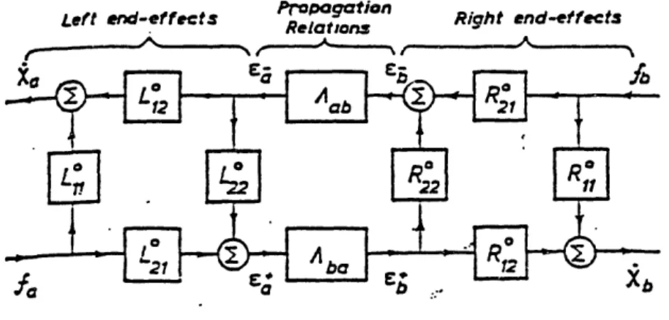
It is somewhat tedious to calculate the fundamental matrix (also known as the transmission matrix) H(s, x) in equation 2.3 by transforming a diagonal matrix of exponentials as in equation 2.9. It is more convenient from the standpoint of control to describe the dyna-mics in terms of propagation and end effects. The physics of wave propagation alnd input admittance are understood more readily when the different mechanisms are separated as shown in Fig. 2.2.

As mentioned previously, te matrix A can be transformned into a diagona.l matrix D

D = T-'AT (2.33)

with

D0

A2 0 0 (2.34)

0 0 0 A4

Notice that the diagonalized matrix D is a complex matrix. It is generally more convenient and easier concept.ually to deal with real matrices. D can be trans-formed into a block diagonal matrix with real components by the transformation

D*= BDB-'

(2.35)

which yields 1 1 0 0 D = O (2.36) 0 0 -1 1 0 0 -1 -1

t ab t M 6

tOa

OD I

4

ax

al 1c dx

o~~~~~~~~~~~~~

oo

Figure 2.1: Transverse forces, displacements, ments of a. thin-beam and differential element

lomenents, and angular

displace-Left nd-effects Propagation _Relations Rght _{Righ nd-c}end-effects

.-- h~~~~~~IA _

Figure 2.2: Propagation and end-effects relations for transverse vibrations of a fiee-free 1beal

Q

1 .I 0 0 1 0 0

-j0

0

0 1 1

o j -j

(2.37) 1 -j o B- 1= 1 1) 01 0 0 1 j

The relationship between the original matrix A and the block diagonal mla-trix D* is

A = TB- 1D*BT -L (2.38)

which may be expressed a.s

A = T*D*T*- 1 which defines the new transforlnation nlatrix T*;

T* = TB-1. This new mlatrix and its inverse are

(2.39) (2.40) p3/2 T* 1 - p3 2 O _13/2 T*-1= °

0

I

0 1 0 V2p) p3/2 p3/2 )-3/2 )p-3/2 p-3/2 )- 3/2 _p3/2 0 1)3/2 0 N/2p 0 p3/2

- v2p

p3/2 _p-3_/2 p-3/2 0 p-3/2 _ V/2p-1 p-3/2 1 A new state vector U may be defined by

Y = T*U.

(2.42)

Plugging equation 2.42 into equation 2.25 along with equation 2.39 yields dU - D*U. dx where (2.41) (2.43) B

This ordinary differential equation nlay be solved between two points a and b where a represents the end of the beaml x = 0, and b represents the end of the

bealn x = 1. The solution to equation 2.43 between a and b is

Ub(p)

elDu,,(p)

(2.44)

with the matrix exponential a block diagonal matrix

D

¢

&VrF

0

e

[

cVFJ

=

(2.45)

0

e-'F

where cos x/~; siII v/~- 1P 2

F=

;

L= .

(2.46)

- sin L Cos v/ 2

Notice that in equation 2.45, the terms containg e4_{V' are not analytic as L -, o}

for large s (the semi-infinite condition). These components cannot be admissi-ble transfer functions (this is the samle argument which led to the equation of characteristic constraint). By letting

U3

i

equation 2.44 can be rearranged so tha.t a. matrix of admissible transfer functions is obtaincd: Aab

t- o

o

~

l)

Ula C(Lp) -S(Lp) a 2l2a - S(Lp) C(Lp) + 2l3b 0 0 eb U t4b 0 0 O O Ulb

C(Lp) S(Lp)

U3a + -S(Lp) C(Lp) U4a Aba (2.47) where C(Lp)=e- ' rL cos v/L S(Lp)=e - '/ ~ sin v\/ Equation 2.47 may be written as

Tile symbols e, eb, Aab, and Aba are illustrated in Fig. 2.2. Vaughan [22] names

the matrices Ab and Ab, as the Bernoulli-Euler propagation matrices, and lie names the operators C(Lp) and S(Lp) prolagationl operators. It is evident tllat these matrices and operators descrilbe p)ropagation within the beam and do not include end effects when it is noted that Aba, which is the transfer fiunction

maltrix between + and , is also the transfer function llatrix between + and E+LI for

1

- 00. Thus, te propagatioll

natrices

describe propagation within the bleamn before any end conditions are encountered.

For free-free 1boundary conditions, equation 2.42 can 1be rearranged to con-form to tile definitions of Fig. 2.2:

L°, 1 V/2- / ' 2 - V1/91 2 1 2p-3/2 0 L2

vp - p

0 2p)3/2 1 -2 0 1 q( ) )2 / fa L22 (2.49) li~b 21~2lt

(t

2

Eb l11j j

1 -_Rp -1 / 2

VI)

) 1/ 2 _{-1 0} 2p-1 -2p 3/2 v/2p- ' ₀ I 2p3/ 2 q f

1

J (

u 3

I

0 24 1 Ro_'21 R22 (2.50) Equation 2.49 describes the end effects of the left, or a end of a free-free beam, and equation 2.50 describes the end effects of the right, or b end. Equations

113

t4 a

I

2.49. and 2.50 may be written in thle sllhort-hlland notation

21 22 a

(

(RL R2 f

)

Now that tile mathelllatical description of a fiee-free beanl has been sepa-rated into propagation and end effects, it is a simpllle matter to study the effect of an arlitary impedance attached to the end of the beam. In the next section,

the effect of attaching a characteristic imlnpedance controller to the right end of the beam is explored.

2.4 End-Point Control of Bending Vibrations

At any point along the length of the beam excepting the end-points, the dynamic variables llust conform to the characteristic impedance, equation 2.32. If a controller is attached to the end of the beaml, it has its own impedance which in general is different from the characteristic impedance of the beam. A terminal ilnpedance may be attached to the right-hand end of Fig. 2.2 as shown in Fig. 2.3. Through the use of block diagram algebra., the attached impedance block can le incorporated into the free-free end effect blocks as shown in Fig. 2.4. The end-effects relations for the system incorporating a terminal impedance are

Rll-=[(I- R°lZb)-'Rl]J

R12=[(I - RlZb)-'R21

(2.51)

R2 1=[RO1(I - ZbRl )-']0

R2 2=R°2 + [R°1(I - ZbR1)-ZbR°2

]

A transfer function matrix may be derived from Fig. 2.4:

b

)

Yba

Ybb

Zb

)

(2.52)

Figure 2.3: Propagation and end-effects relations for free-free beam with termi-nal impedance appended

Figure 2.4: Propagation and end-effects relations for beam with terminal impedance incorporated into end-effects

Y,,=L

°

_{i + L}

2

(I

-

AbR

22

AbaL°2

)-'

1

AbR

22

AbaL

y~~b=LO2(i a Ab.R22Ab L22 )

a-

b2Ab.LR2

Yb=L1 ₂(I -12\" -'22 AR _{2 2}AbqL° )l ) AbRab ₂1

(2.53)

Yba =R1 2(I - ta L 2A,,bR22)- 1Ab L°l

Ybb=Rll

+

R12( I- AbaLuR 22 )- Aba LAabR21

By examining Fig. 2.4, it is evident that if R22 could 1be made identical to

0, there would be no reflections of waves propagatillg from left to right. This describes the behavior of a semli-infinlite beam as described in Section 2.2 which suggests the use of the beam's characteristic impedance givei by equation 2.32 for a. terminal impedance, i.e.:

(

)b

=

I(

IG

2

)

)

(2.54)

q b =

K~,-,;2

c-) - b'

where the *-ed variables are reference values. In particular, if Zb is equal to the characteristic impedance of the beam (i.e., GQ = G =/': = K = 1), then the reflection matrix R22 is identical to the zero matrix which means that no wa-ves

are reflected from the right-hand end of the beam. Thus, enforcing the equation of characteristic constraint at the end of the l)eanl does make the beam behave as a semi-infinite beam.

2.5 Boundary Conditions

Equation 2.52 is the transfer function matrix for a distributed parameter beam with the left-hand end free, and the right-hand end ternlinated with an imped-ance. The appended impedance may describe a control, or passive end condition (i.e. pinned, clamped, sliding, etc.), or both. For a more general description of a. beaml terlinal impedances may be a.lpellded to both ends of the beam model so that Equation 2.53 becomes

Yaa=LII + L_{1 2}(I - AabR22AbaL22)-AabR22AbaL21

Yb =L2(I - AabR22AbL22)-'AabR21

(2.55)

Yba=Rl2(I - AbaL22AabR22)-1AbaL2l

Ybb =R, + R_{1 2}(I - AbaL22AabR22 )-1AbaL22AabR1

with

Lll=[(I - LtZ, )-' L°

₁

]

L12=[(I - L Z )-I'L1 1 1212

]

(2.56)

L

21

=[L°(I - Z,,Ll )-']

L

22

=L2 + [L°(I - ZLi)-lZ.L

].

2

Using this approach, the transfer function mlatrix mllay be found for a variety of bea.m configurations.

2.5.1

Clamped-Free Beam

One of the cases studied in this paper is the cla.mped free beam. This case is of particular interest because since both linear and angular velocity is present at the beam's end, the full end point impedance controller imay be implemented. The clamlllped-free condition nay be implemented with a cantilever beaml witih the left end clamped, and the right end free, as shown in Fig. 2.5. The geometric

l)oundary conditions at the left-hand end are y(t) = 0 and 0(t) = 0. These boundary conditions can be plugged into equation 2.42 to yield

0\

r2p(uI

+

U

3

)

1 2 11= + 2 -- 113 + 114) (2.57)

q

2 3 112 - 14)

a - (-111 + 112 + 113 + 114) which may be solved to eliminate n and q:

ea

{U4 a -[2 1 U2 a(2.58)

By examining equation 2.49, it is seen that equation 2.58 is in the form e+ ₌

L22e. L, L12, and L21 are all equal to O. Plugging these values of Lij, and

Rij = Rpj into equation 2.55, the transfer function matrices for the clamlped-free beam configuration are

Yaa=O

Yab =0

(2.59)

Yba =0

The transfer fnction matrix Yht, is a 2 x 2 matrix of transfer functions and mnay be written as

Ybb Y= l,(2, 1) Y Yhh(2, 2) (2.60) Using the values for the R fonl eluation 2.50, and tile value of L22 from equation 2.58, the elements of the transfer finction matrix Ybb can be calculated:

Ybb(1, 1) = + C + 2 - + 1 (2.61) (S2 + C'2)2 + 252 + 6C2+ 1 Ybb( 1

2 )

(S2 + C, )2 + 4SC - 1 (2.62)

Ybb(,

2

₎

_{= (52}

_{+ C)2 + 2S2 + GC'2}

_{+ 1}

_(2.62)

(S

+ C')

- 4SC - 1

Ybb(2, 1) = - P ( + C) + 2 + C2 + 1 (2.63) (S2+ C'2₎2_{+ 2S 2C} 2_{+ 1} Ybb(2, 2)

_{(S + C2) + 2S + 6C + 1}

+ 22 + 2S +

C

2

+

1 (2.64) where

S S(Lp) =-e-lVrfi

sinj

L =

--C'C'( Lp)=e- ¥ cos v/T ' 2

The above transfer functions model the beliavior of a clamped-free beaml and include all modes. The approximation of these transfer functions is discussed in

Chapter 3.

2.5.2 Clamped-Sliding Beam

A beam configuration which may be used to model a Remote Center Compli-ance is a clamped-sliding beam configuration. As shown in Fig. 2.6 the left-hand boundary conditions are the same as that for a clamped-free beam, but at the right-hand end, (t) = 0. These boundary conditions can be plugged into equa-tion 2.42 to yield 2 p(ll + Ul3) 0

J

(ll + U2 --t' U3 ₄ ) (2.65) m7 = A~-lp(U2 - U4)

L,

(

~

3

(--

2 1

1

1U3 1

4

)

Jb

Figure 2.5: Clamlped-Free beam configuration

y=O

0=0

Figure 2.6: Clamped-sliding beall configuration

8=0

which may be rearranged to forlll ll2 k u 11 Ri!

--

O -LXp/2

_o

₂

0 0 0 _-)3/2 0 p-)3/2 RI2 \/-1) 0 0 o0l o1

I

0 -i

Plugging these alues of Rij along with tile value of L22 into equation 2.55, the transfer function matrices may be calculated. As in the clamped-free case,

Yaa = Yab = Yba = 0. The transfer function matrix relating output to input at the right hand end is

Ybb = R11, + R12(I - AbaL22AbR 22)-'AbaL 22AabR2I (2.67)

which may be expanded into its four collponellt transfer functions. of a. clamped-sliding configuration, Ybb( 1, 1) = Ybb(2, 1) = Ybb(2, 2)

Y1 2) = (S 2 + C2)2

-

G S - 2C'2+ 1 Ybb(l 2)-

4SC1

In this case = 0 and (2.68) where

S-S(Lp)e

- /

_sill

_{v L}

_{-- 12}

C'-C(Lp)=e -V cos V '

2-This is the transfer fiulction between a force input, and linear velocity output at the right hand end. Because of the (t) = 0 constraint, an applied moment has no effect, and an applied force does not induce a. rotation.

The approximation of the transfer function for the clamped-sliding beam will be discussed in the next chapter.

77 q 113 U(4 b (2.66) I

Chapter 3

Dynamic Simulation

3.1 Approximating Infinite-Order Systems

Models for distributed parameter systems describe ifillite order systems as op-plosed to lumped parameter systems which are modeled with a finite number of energy storage elements. If a closed-forml, tinle-cloniain solution of the system transfer function matrix 2.52 can be found, then the theoretical time response call be calculated exactly. However, a closed-form, timle-domain solution mlay be impossilble to find. Therefore, an approximlation of the time-domain response is sought.

As an exampllle, equation 2.52 is the transfer function imatrix for a free-free bealn with a controller attached to the right-hand end. The third of equation 2.53, Yb, is a transfer function matrix of the velocity outputs of the right-hand end of the beam to the disturbance force and moment of the left-hand end of the beam. The elements of Yba may be written as:

4S(S

2

_{+ C}

2

_{- 1)}

Yba(l, 1) 2 + C's2 6S2-2 C 2 + 1 (3.1)

(S

2

+

C

22

)

_-

_6S2

_{_ 2C}

2

_{+ 1}

Yb

, -

p s___.(

S + C)(

S

₊

2

_C

2)

_{+ (S}

_-

_C)

_(3.2)

Yba(2, 1)= 2 (S2 + C2)2 _S2- 2C2 + 1 (3.3) 4S( S2- C2 - 1) Yb(2, 2) _{(S2 + C}2₎2 _{_ 6S}2_{- 2C2 + 1}= (3.4) where

S=S(Lp)=

-~

_sill

_L-

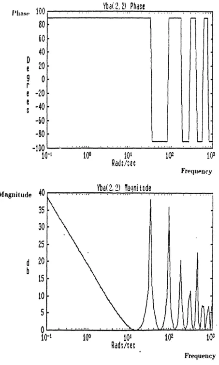
12--C'=C'(Ll))=t-4cos V/T j;' 2

Tlhese transfer functiolls are transcenldental and have infinitely mnany ploles and11(1 zeros. A closedi forin solution of these transfer functions via, the inverse lal)lace transforml was not a.ttellllte(l. Instea(l, a Pade type approxima.tion wa.s nla(le to create a. polynomial transfer function. The alpproximation wa.s made by first constructing a Bode plot of the transcendental transfer function. By way of example, the ]beaml used b)y Vaughan [22] is used to demonstrate the digital simulation of a free-fiee beam. The paranleters for this example beaml are given in Table 3.1. A Bode plot for Yh,(2,2) using these paranleters is shown in Fig. 3.1. The first five poles and zeros as well as te appropriate gain were then estimated fron te Bode plot. A more p)recise estimate was obtained with the use of a zero-finding IMSL routine(ZANLYT). Te first five pairs of poles and zeros were estimated and are shown in Table 3.2. The estimated poles, zeros, and gain were then combined to form a transfer function of tile form

Gain

((s/-Z

)

+ )

((s/-

2

)2 +

((S/z

5

)2 +1)

Yb (2, 2)= (3.5)

( ((s/ )

2

+ 1) ((/P2) 2 +

1)

((q/p))

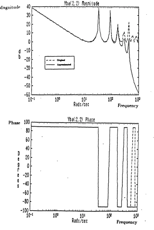
+ 1) which could then be converted into a conventional state-space representation.

A comlparison of the Bode plots of the approximated transfer function and the original transfer function is shown ill Fig. 3.2. The fidelity of the approximla-tion is excellent up to the third mode, after which the approximated transfer function rolls off in magnitude. The approximation is expected to roll off in the higher frequency range because the approximation is only for the first five modes. However, there was more attenuation at the fourth and fifth mode than was ex-pected. This does not rea.lly cause any problems because for the cases studied, these higher modes contribute only a. small amount to the velocity signals and are well daimped.

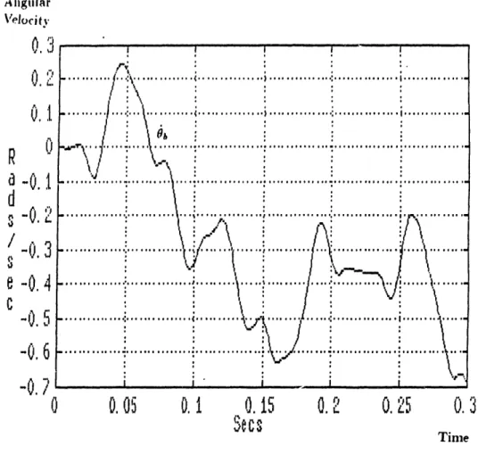
The time domain solution of the approximated system may be easily solved for an arbitrary input using comercially ava.ilabel software packages such as CTR.L-C or PC-MATLAB. Fig. 3.3 shows the response of b to a ten pound step in Q, for an uncontrolled free-free beam. The fractional operators used in the controller were also approximated using a Pade type approximation. The method used to derive the approximation differs from that used above for finding

Length (I)

Cross-section area. (4) Young's modulus (E) Density (p)

Area moment of inertia (I) a = E/ IpA)

EI/a

30 x 106 l1 0.725 x 1 0-3lb-sec2 in. 0.0796 in.4 57.5 x 103 in._sec 41.5 in.-lb (in./sec)

Table 3.1: Example bea.l parallleters

Gain = -. 4589

Poles

Zeros

0 ±32.16i ±28.40 ±88.65i ±113.5 ±173.8i ±255.4 I287.3i I454.0 ±429.2i ±709.4

Table 3.2: Poles, Zeros, and Gain for Yb,(2, 2)

200 in.

too o10 102

Rad:/,ac

o10 10' 102

Rads/se:

Frequency

Figure 3.1: Bode plot of Yb,(2, 2)

[,I.e IDO 80 60 40 D e 0 9 0 r e -20 e -40 S -60 -80 _inn -iAvv Magnitude 40 35 30 25 d b 20 15 103 Freqiency 103 10 5 n

to-M ag;lnit.ludle 40 30 20 10 0 d -10 b -__-Lo -40 -40 -50 -h, Phase 10I 80 60 40 D e 20 9 0 r e -20 s -40 -60 -80 -1 fl io-I i 10 101 102 10 Rads/sec Frequency 10"- 10° 101 i02 I0 Rads/se C Frequency

0. I 0.)15

SeCs

0. 25

Figure 3.3: Response of 8b to step input in Qa Angular \'eloci ty 0. 1 ci2 R 0 a -O. 1 d s -0. 2 / -0. 3 e -0. 4 -0. 6 (

.. ..

... ...

...

... ... .. . .. .. ... .I . . . ....

I

.. . .

I.

· 111111111 @1· 111111 111111 ,·1Ill·~~· ~ ~·· ~ 1~1·· e· 11I

0. 3

Time

al)l)roximlations for the systenl transfer functions. Appendix A describes tle alp)lroximlation of the fractional operators.

3.2 Control Simulation of Free-free Beam

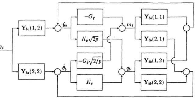
Using the model developed in the previous section, the effects of the controller of equation 2.54 may be included. A block diagram of the free-free beanl with the controller attached is shown in Fig. 3.4. The locks for 1,(1,2), 1,(2,2),

lbb(1,2), and lbb(2, 2) were implemented digitally using forward integration (Adamls-Ba.shford)[20]. The blocks for lbb( 1, 1) and lbb(2, 1) were imllemented using backward Euler integration due to the "stiffness" of those transfer func-tions(see Appendix B). A software package such as TUTSIM allows seperate bllocks to be linked together easily. By adjusting the values of the coefficients Gy, G,, IK, and KI, different control cnfigurations can be formed. By letting these coefficients be all equal to 1, the controller takes on the form of the beamns characteristic impedance, as described in Section 2.4. Fig. 3.5 shows the time re-sponse of the free-free beam with the same conditions a.s for the rere-sponse shown in Fig. 3.3.

3.3

Simulation of Clamped-free Beam

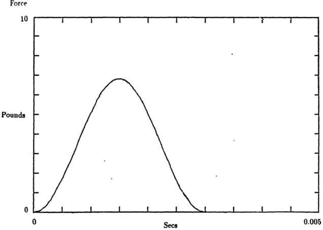
The first beam configuration used for experilllentation described in the next chapter is the clanmped-free beam. The parameters used for the simulation are given in Table 3.3. Fig. 3.6 shows the block diagram for a clamped-free beam configuration including the controller. The blocks }bb( 1, 1) and l}bb(2, 1) were im-plemented using backward integration due to the stiffness of the system. Fig. 3.7 shows the uncontrolled time response (controller gains set to zero) of the beam's linear tip velocity to the force pulse shown in Fig. 3.8, which approximates the pulse imparted to the beam by an impact hammer. The plot in Fig. 3.7 is the response to a pulse input with a pea.k force of ten pounds, a.nd a duration of three milliseconds.

By setting the appropriate gains to zero in the controller matrix (equa-tion 2.54), several different controllers can be constructed. By setting KI = 1, for example, and the other three gains to zero (KI control), the same input

Figure 3.4: Free-free beam with controller: block diagram Angular Velocity 0.5; Rads/sec -0.5 0 _Secs

Figure 3.5: Response of free-free beam with controller attached

0.3 Time

Length (1)

Cross-section area (A) Young's modulus (E) Density (p)

Area. moment of inertia (I)

a = EI/(pA)

Ella

11 x 106 11) n111. 0.266 x 10- 3lb-sec2 ill. 0.97G x 10-3 iln.4 7.35 x 103 i.2_$ec il.-ll)

(ill./sec)

Table 3.3: Clanmped-free beamn parameters

Figure 3.6: Block diagram for clamped-free beam

52 ill. 0.75 in.2

O Sees

Time

Figure 3.7: Linear velocity response to force input: uncontrolled Linear

Velocity

in/sec

-5M

Force 10 Pounds O 0 _0.005 Sees Time

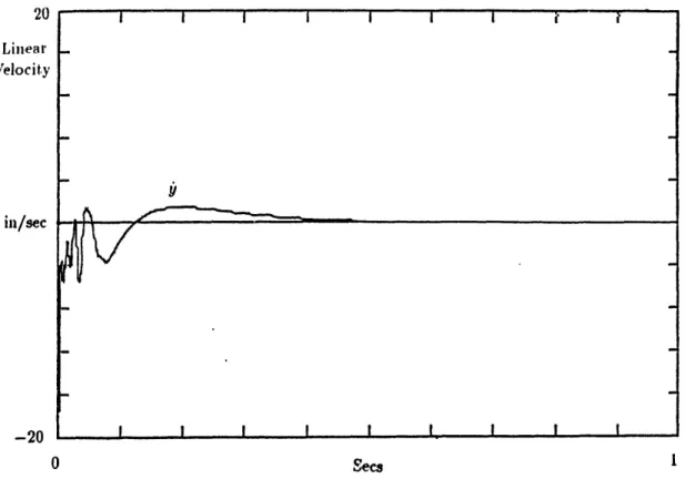
used for Fig. 3.7 produces the response shown in Fig. 3.9. With I;K6 = Ki = 1 and the other two gains equal to zero(A control), the response becomles that shown in Fig. 3.10. Fig. 3.11 shows the response of the clamped-free bleam with a characteristic illedance controller (all gains set to 1 (Z control)).

3.4 Simulation of Clamped-Sliding Beam

The beaml configuration which emulates the motion of the Rellote Center Coln-plia.nce is the clamped-sliding l)ea.nl. The results of Chapter 2 show that there

is a single transfer function for a clamped-sliding beaml, lbb( 1, 2), which is the

transfer function between a force input and linear velocity output. A set of para.meters consistent with the beam used for experiments is summarized in Ta-1ble 3.4. A simlulation of the response of a. clamped-sliding beall to a pulse input (8.5 pound peak force) is shown in Fig. 3.12.

Because of the absence of any angular motion at the tip of a clamped-sliding beanm, it is not possible to implement the complete control law Equation 2.54. The only element that can do any work is I4 Jv/~ so that the control law for a. clamped sliding bea is

qb = IO /2p~Y (3.6)

Using IK = 1, the uncontrolled simulation of Fig. 3.12 is transformed into Fig. 3.13. Even without the full impedance controller, it is possibie to do effective dlisturbance rejection for the clamped-free case.

I

Time, Secs

Figure 3.9: Clamliped-free beani with I control

Length (1)

Cross-section area (A) Young's imodulus (E) Density (p)

Area mloment of inertia (I)

a = EI/(pA)

El/a

10.75 in. 0.02 in.2 30 x 106 lb in. 0.725 x 10- 3 b-sec in. 0.667 x 10- 6 in.4 1.18 x 103 in_sec -017'- in.-lb .0 in./sec)

Table 3.4: Clanmped-sliding beam parameters

20 Linear Velocity in/sec -20 0 I I I I I I I i . ! !L I! I I !, I I I .. o

Li lea.r Velocity 20 20 I I IIII I t i in/sec -20 I 11 0 Secs 1 Time

Linear Velocity 20 . i l 1 1 - l ia in/sec -20 I I 1 I L I I I I 0 _Secs 1 Time

Linear Velocity 800 in/sec -800 0.5 0 Ses 0. Tinpute

Linear Velocity 800

ill/sec

A

-800 X X X 1 1 l l l 1 0 0.5 Secs Time

Chapter 4

Experimental Analysis

In order to study the effects of the end point impedance controller, two experi-ments were conducted: a clamped-free beam experiment so that all four eleexperi-ments of the impedance controller could be implenlented; and a clamped-sliding beam experiment so that the active damping of a Remote Center Compliance model could be demonstrated. The two experiments required seperate setups which will be described individually.

4.1

Clamped-free Beam

4.1.1 Experimental Setup

The parameters for the beam used in the clamped-sliding experiment are listed in Table 3.3. The beam was clamped to a large Contraves air bearing table using steel angle brackets as shown in Fig. 4.1. The air bearing table was not floating during the experiment and it was clamped so that it could not rotate. This was important because if the clamped end of the beam not held rigidly, the clamped-free model would have been invalidated. The beam was horizontal so that there were no non-linear stiffening effects due to gravity.

Motion of the tip of the beam was measured through the use of a linear ac-celerometer and an angular acac-celerometer. The angular acac-celerometer (Endevco model 7302-B) was rigidly attached to the tip of the beam via an aluminum bracket which was bolted to the beam. The linear accelerometer (Entran model EGA-125-5D) was mounted to the same bracket as the angular accelerometer by bonding it with bee's wax. Both accelerometers were piezoresistive and were

balanced using a Vishay strain gauge conditioner. The Vishay had a base gain of 100 with an additional adjustalble gain. Tile gain for tile angular acceleration signal was set to 20 for a total gain of 2000 in tile Vishay, and the angular acceleration signal had a gain of 10 for a total gain of 1000. The angular ac-celeronleter had a. sensitivity of 3.5 and tile linear accelerometer had a

ra.cl/sec

sensitivity of 11.95

n

,. in/sec

Tlhe acceleration signals fronm the Visllay strain gauge conditioner were in-tegrated using analog circuit integrators which included a high pass filter to ac-couple tile signals. This elilinated ally dc comllponent due to drift of the Vishay. The controller was also built with analog components. The fractional operators were built using operational amplifier circuits as described in Ap-peldix A, and they used ten-stage lattice networks in the feedback path. The valid frequency range for the /; operator was 18 hz which is high enough to include the first two modes of the beam. The operator for /lis was imple-mented with smaller values for the resistors and capacitors in order to boost the gain for this operator. This also increased tle bandwidth of the fractional integrator to several thousand hertz. The reason for such a large improvement

in performance is not understood. The same values of resistors and capacitors

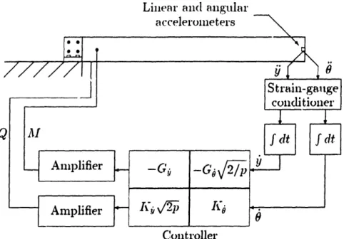
were not used in the fractional differentia.tor because high frequency noise would have been amplified. The products of all the system gains were calculated and lumped into the four controller gains. These gains are given in Table 4.1. These gains include the gain of the Kepco amplifiers (Model BOP 1000M) which was 100. The gains also include tle gains for the filhn actuators. The calculation of the actuator gains is described in Appendix C. The moment actuator had a gain of 9.937 x 10-5 in lbf/V. The force actuator had a gain of 9.0 x 10- 7 _lbf/V.

Notice that the controller gains needed to match the characteristic impedance at the end of the beam are G = G =

KI

=

KI;

= 1. The gains used in tle controller were limited in magnitude because of the small gain of the film actu-ators. Voltages applied to the piezoelectric film were limited to ±400 volts by using zener diodes in the controller circuitry. This was done because too high a voltage would destroy the piezoelectric filmn.

All measurements were taken with a Nicolet Dual Channel FFT Analyzer (model 660B) which was connected to a Tektronics digital plotter (model 4462).

Linear and angular

Controller

Figure 4.1: Side view of clamped-free beam setup

Gj=0.01282 G0=166.2 x 10-6

KI=0.0071

KI=287.35

x 10- 6

4.1.2 Procedure and Results

All the data collected froml experilmenta.tion with the clamped-free b)ea.n wds restricted to the time domain. Tile calculation of fiequency donla.in transfer functions was attempted via. impact testing. However, the sharp pulse produced by a hlamllner imlpact caused current srges that were harmfiul to the piezoelectric

film. For this reason, impact testing was abandoned, and tests were restricted

to initial displacenment decays except for several time domain decay excited by a light impact.

For the initial displacement tests, the tip of the beam was displaced one inch and released. This type of input mainly excited the first mnode of the btuam. Fig. 4.2 shows the linear tip acceleration signal produced for a. free decay with the controller unattached. The end point impedance controller was then attached so that both a control force and a control moment would be applied to the end of the beam. Fig. 4.3 shows the linear tip acceleration with the controller attached. In order to study the sepera.te effects of the control moment and the control force, first the control force was disconnected so that only a. control moment was applied (G-control); then the control moment wa.s disconnected leaving only the control force (K-control). Fig. 4.4 shows the response of the linear tip acceleration to an initial displacement with the control moment applied, and Fig. 4.5 shows the response of the linear tip acceleration to a initial displacement with the control force applied.

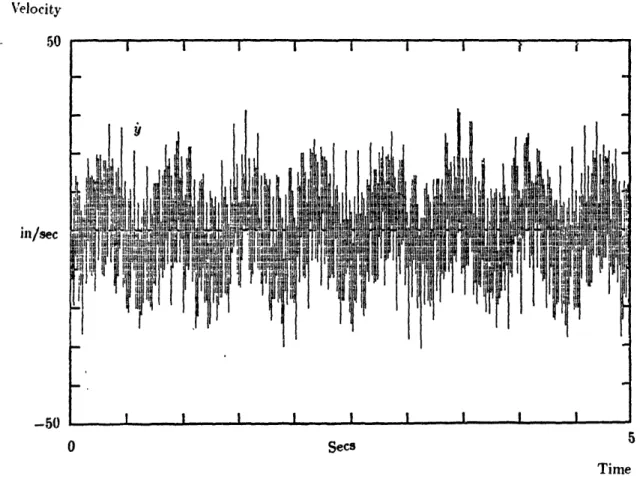
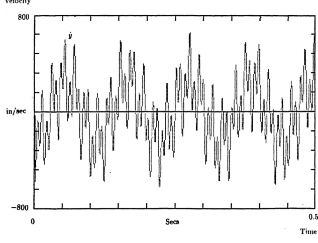
In order to demonstrate the active control of more that one mode sinmulta-neously, ai impact test was done using a very light hit so that the film would not be damaged. The result of the impact was to excite multiple modes at once. A typical force pulse is shown in Fig. 4.6 with a magnified time scale so that the pulse shape details are visible. The typical force pulse had a duration of 0.005 seconds and a peak magnitude of 0.8 pounds. Fig. 4.7 shows the response of the linear tip acceleration to an impact with the controller unattached. Fig. 4.10 show the response of the linear tip velocity of the clamped-free beam to a.n impact.

The end point impedance controller was then attached and the tip of the beamn was again impacted. Fig. 4.8 shows the controlled response of the linear tip acceleration to an impact. Fig. 4.9 shows a simulation of the response of the

Linear Acceleration

48.5

in/sec2

-48.5

FREE PECAy FRQM IN.ITIAI DI$PLA.EMENT

H 0

._

I I I I I I U I I f

_I

I I I I I i ! I I I SEC Time

Figure 4.2: Free decay from initial displacement for clamped-free beam

DISPLACEMENT

i 48.5 Linear Acceleration in/sec2 -48.5 0 F ·I - -I I I

SEC

200

Figure 4.3: Controlled decay from initial displacement for clamped-free beam II *ULL CONTROLLER

TIP ACCELERATION

:AR . . I I a a I Time _ - --- -C---Y CONTROLLED I

DECAY FROM

INITIAL

i I I I

i

DISPLACEMEN

48.5 Linear Acceleration ill/see2 -48.5 I I I - I II 0 SEC Time

Figure 4.4: G-control of clamped-free beam G-CONTROL ACCELERATION I -I -_ I___ I I I _ X w l-

---r---

_I-C

--- -- C

- ~ CONTROLLED

F

L DECAY FROt I

1

INITIAL

lI_ R TIP I Z~ I I

Lilea Accelerat il/se -48.5 Figtre 4.5: It-contrlo l of Time lallpecl-free beam

FORCE PULSE

a I .

SEC

0.04

Time

Figure 4.6: Typical impact pulse applied to clamped-free beam

Force 1.04 Pounds -1.04 0 j I _1 * I I I J~~~~~~~~~~ __ _ __ _ I L .I I

Fo. Potl Lin Accele ill, U.21 rce nd-0.21 -0.21-ear ration -/9ec2 q).3 I I IJ..; I ; _

FORCE

PULSE

0 i I I I I I

SEC

20

Time

Figure 4.7: Uncontrolled impact response of clamped-free beam

A I .UIN ~~~~~~~~~mM

I- I -. ' . I i.

UNCONTROLED IPIPACT RE§PCNSE

" "'

L

mm

S.