A 32 sub-band/transform coder incorporating vector quantizing for adaptive bit allocation

A 32 SUB-BAND/TRANSFORM CODER INCORPORATING VECTOR QUANTIZING

FOR ADAPTIVE BIT ALLOCATION

by

Courtney D. Heron

Submitted to the

DEPARTMENT OF ELECTRICAL ENGINEERING AND COMPUTER SCIENCE in partial fulfillment of the requirements

FOR THE DEGREES OF BACHELOR OF SCIENCE

and

MASTER OF SCIENCE at the

MASSACHUSETTS INSTITUTE OF TECHNOLOGY February 1983

(c) Courtney D. Heron, 1983

The author hereby grants to MIT permission to reproduce and to

distribute copies of this thesis document in whole or in part.

Signature of Author ... SC-- IV. . X-. ea-... .· . . . ... Department of Electrical Engineering and Computer Science,

October 8, 1982.

Certified

Certified

by

... ;

.a...:

_{hvnesis Supervisor (Academic)}

...

by . .

C ompa Wuperv k1, s

o

pang

Accepted

by_

...

...

. . .

...

Chairman, Departmental Committee on Graduate Students

Archives

MASSACHSETTS INSTI983TUTE

'MAY 2 7 1983

LIBRARIES Company) . .. l. .... ... ...

A 32 SUB-BAND/TRANSFORM CODER INCORPORATING VECTOR QUANTIZING

FOR ADAPTIVE BIT ALLOCATION

by

Courtney D. Heron

Submitted to the Department of Electrical Engineering and Computer Science February 1983 in

partial fulfillment of the requirements for the Degrees of Bachelor of Science and Master of Science in

Electrical Engineering

ABSTRACT

Recently frequency domain techniques for coding digital voice have received considerable attention. Sub-band coding (SBC) with 2 to 12 frequency bands and a relatively low computational complexity is at one end of the scale. Adaptive transform coding (ATC) with 128 to 256 bands and relatively high computational complexity is at the other end of the scale. At coding rates of 16 kb/s ATC is generally rated to be superior in quality to SBC. In this thesis the middle range of complexities and channel bandwidths between those of SBC and ATC have been investigated by experimenting with new techniques for 32 band sub-band/transform coding at 16 kb/s. Dynamic bit assignment and adaptive quantization of the sub-band signals have been accomplished with a new spectral side information model consisting of a switched source of all-pole spectral templates in accordance with recent concepts of vector quantizing and clustering methods. Two new designs for 16 kb/s 32 band sub-band/transform coders which were simulated on a general purpose digital computer are presented.

Informal listening tests were carried out to compare the quality of these coders with previous SBC and ATC designs. The coders were also compared on the basis of computational complexity. The overall results appear promising, indicating that the new coders have a quality similar to ATC with about three times the complexity of 4 band SBC. Suggestions are made for further research of these middle range techniques.

Academic Thesis Supervisor: Dennis H. Klatt Title: Senior Research Scientist

Company Thesis Supervisor: Ronald E. Crochiere Title: Member of Technical Staff, Bell Laboratories

ACKNOWLEDGMENTS

I wish to express my sincere gratitude to my advisor at Bell Laboratories, Dr. Ronald E. Crochiere, for his guidance, encouragement, and helpful suggestions. Further special thanks is due to Dr. Richard V. Cox for his continued advice and enthusiasm. His assistance in software development and in the learning of the computer system has been invaluable. I owe special thanks to Dr. Lawrence R. Rabiner for providing the software for the clustering algorithm used for generation of the spectral templates. I am also particularly indebted to Dr. James L. Flanagan of Bell Laboratories for inviting me to work in his department and for providing all the necessary facilities, and to Dr. Dennis H. Klatt of MIT for agreeing to be my thesis supervisor.

I would like to thank Dr. Ronald E. Crochiere, Dr. Ronald E. Sorace, Dr. Richard V. Cox, and Dr. Dennis H. Klatt for their helpful and thorough comments on earlier versions of this manuscript. Special thanks is also due both the the Word Processing and the Drafting Departments of Bell Laboratories for their fine work.

I would like to thank the National Consortium for Graduate Degrees for Minorities in Engineering for their fellowship support. I am also grateful to John Tucker and the MIT 6-A program for giving me the wonderful opportunity to work for Bell Telephone Laboratories.

Finally, I am sincerely thankful to my parents, Ivanhoe and Violet Heron, for their continuing love, support, and encouragement.

TABLE OF CONTENTS

TITLE PA G E ...

A BSTRA CT ... ... ... 2

ACKNOWLEDGMENTS

...

3

TABLE OF CONTENTS ... 4

LIST OF FIGURES AND TABLES ... 6

I. INTRODUCTION .... ... 9

1.1 A Brief Description of the 32 band sub-band/transform coder algorithm ... 13

1.2 The Scope of the Thesis ... 16

II. A 32-BAND QUADRATURE MIRROR FILTER BANK IMPLEMENTED WITH A PARALLEL STRUCTURE ... 18

2.1 Introduction ... 18

2.2 Principles of Tree Decomposition ... 18

2.3 Derivation of the Parallel Structure from the Tree Structure ... 20

2.4 The Implementation ... 25

2.5 Filter Bank Transfer Function ... 26

2.6 Observations ... 27

III. A SPECTRAL SIDE INFORMATION MODEL FOR SPEECH SIGNALS ... 29

3.1 Introduction ... 29

3.2 Derivation of the Spectral Templates ... 29

3.2.1 The clustering algorithm for generating the templates ... 30

3.3 A dynamic Template Selection Scheme ... 31

3.4 An Evaluation of the Tradeoffs between the Spectral Accuracy and Complexity of the Template Model ... 34

3.4.1 Observations ... 37

IV. A BIT ASSIGNMENT SCHEME FOR SPECTRAL NOISE SHADING ... 40

4.1 Introduction ... 40

4.2 Bit Assignment for Flat Noise Power ... 40

4.3 Bit Assignment for Noise Shaping ... 42

4.4 Observations ... 48

V. ADAPTIVE QUANTIZATION OF NARROW BAND SUB-BAND SIGNALS ... 49

5.1 Introduction ... 49

5.2 A Review of Adaptive Quantization Schemes for Frequency Domain Speech Coding ... 50

5.3 An Adaptive Quantization Scheme for Coding the Outputs of the 32-Channel

Analysis Filter Bank ... 58

5.3.1 Observations ... 66

5.4 A dynamic Pre-Emphasis/De-Emphasis Scheme for Adaptively Quantizing the Outputs of the 32-Channel Analysis Filter Bank ... 67

5.4.1 Observations ... 71

VI. AN ANALYSIS OF THE PERFORMANCE AND COMPLEXITIES OF BOTH 32 SUB-BAND/TRANSFORM CODERS ... 73

6.1 Introduction ... 73

6.2 Results of an Informal A versus B Comparison Test ... 73

6.3 The Complexity Performance Trade-offs ... 77

VII. SUMMARY AND RECOMMENDATIONS FOR FURTHER RESEARCH ... 81

7.1 Summary ... 81

7.2 Suggestions for Further Research ... 81

REFERENCES . .. ... ... ... ... 83

APPENDIX I QUADRATURE MIRROR FILTERING ... 86

APPENDIX II FOURTH ORDER LPC TEMPLATES FOR 1,2,3,4, AND 5

BIT CODEBOOKS

...

...

98

APPENDIX III THE BIT ASSIGNMENT USED FOR GENERATING THE BIT ASSIGNMENT CODEBOOKS ... 105

APPENDIX IV THE D.S.P ... ...108

LIST OF FIGURES AND TABLES

FIGURES

1.1 Block diagram of a sub-band coder ... 1 1.2 32 band sub-band/transform coder algorithm ... 13 2.1 2 band QM F filter bank ... 19 2.2 Tree structure implementation of a 32 band QMF

filter bank ... 21 2.3 Parallel structure implementation of a

32 band QMF filter bank ... 22 3.1 Flowchart of template generation procedure ... 32 3.2 Relationship between the accuracy and complexity

of the spectral side information model ... 36 3.3 Superimposed input and template spectra

for two complexity extremes ... 38 4.1 Bit assignment rule for a flat noise spectrum ... 43 4.2 Example template and derived bit assignment

for a flat noise spectrum ... 44... 4.3 Frequency weighted bit assignment rule ... 46 4.4 Bit assignments and quantization noise for

flat noise spectrum and for flat SNR ... 47 5.5.1 General feed forward adaptive quantizer with

a time-varying gain ... 51 5.1.2 General feedback adaptation of the

time-varying gains ... 52 5.2 Block diagram of LPC vocoder driven adaptive

transform coder ... 55 5.3 Block diagram of a modified LPC vocoder

driven adaptive transform coder ... 56 5.4 Homomorphic side information model ... 57 5.5 Illustration of the quantizer output ranges

and input levels for 8 template 4th order

LPC modelling ... 61

5.6 Illustration of the increased accuracy of coding with a 32 template 10th order LPC side

information model ... 62 5.7 Distortion Performance of vector quantizing for

a 1024 template 10th order LPC analysis ... 64 5.8 Subjectively optimized quantizer output ranges

and input levels for 32 template 10th order

5.9 32 band sub-band/transform coder algorithm

with dynamic preemphasis ... 68

5.10 Subjectively optimized quantizer output ranges of preemphasized input levels for 32 template 10th order LPC modelling ... 70

5.11 Illustration of quantizer underloading' and overloading ... 72

6.1 Assessment of coder performance versus complexity ... 79

I. 1 Composite frequency responses of the 32 band-pass QMF filters ... 96

I. 2 Magnitude ripple of the 32 band analysis/synthesis filter bank ... 97

II. la 1 bit 4th order LPC template codebook ... 99

II. lb 2 bit 4th order LPC template codebook ... 100

II. Ic 3 bit 4th order LPC template codebook ... 101

II.ld 4 bit 4th order LPC template codebook ... 102

II. le 5 bit 4th order LPC template codebook...103,104 III. 1 Flowchart of the bit assignment rule for a fiat noise spectrum ... 106

TABLES 6.1 Percent preference of coders in an

informal A versus B Comparison Test ... 75 6.2 Ranking of coders according to the

percent of A versus B votes received ... 76 I.1 Z-Transforms of Analysis Filters ... 89 1.2 Filter coefficients, Frequency Response,

and QMF Ripple for the filters HI(z),

CHAPTER I

1. INTRODUCTION

Recently, there has been considerable interest in applying digital technology to a broad range of applications in communications and coding. This technology offers important advantages such as flexible processing, increased transmission reliability, and error resistant storage - to mention a few. A variety of digital signal processing techniques, which exploit known properties of speech production and perception to varying degrees, has been proposed and studied for the purpose of reducing the required transmission bit rates or storage requirements for such "digital voice" applications [1]. These signal processing techniques range from low to high computational complexity designs which offer a corresponding tradeoff between complexity and performance.

Historically, speech coders have been divided into two broad categories, waveform coders and vocoders. Waveform coders attempt to reproduce the original speech waveform in accordance with some fidelity measure whereas vocoders model input speech according to a speech production model that separates the sound sources and vocal-tract filtering functions for resynthesizing the speech. Waveform coders have been more successful at producing good quality, robust speech, but require higher bit rates (in excess of 8 kb/s). Vocoders are more dependent on the validity of the speech production model and tradeoff voice quality for lower bit rates (2-5 kb/s) [1-2].

In order to reduce the bit rate of waveform coders, much effort has been devoted to frequency domain methods where the speech is encoded separately in different frequency bands. These methods permit control over the number of bits/sample and therefore the accuracy that is used to encode each frequency band. This enables different bands to be encoded with different accuracies according to their information content. The basic systems which have been studied extensively are sub-band coding and transform coding.

Sub-band coding, which exploits the quasi-stationarity and non-uniformity of the short-time spectral envelope of speech, is based on a 2 to 12 band division of the speech spectrum by means of a filter bank. In this scheme the number of bits/sample allocated for quantizing each frequency band is fixed at a certain value. The quantizer step sizes in each band are independently self-adapted according to a first order predictive technique after Jayant [32] which exploits the sample-to-sample amplitude correlation in each band. In general sub-band coding offers moderate complexity with moderate quality.

Transform coding, which exploits redundancies in the short-time speech spectrum, is based on a 128 to 256 band division of speech by means of a block transform analysis [2,31. In this technique the input speech is blocked into frames of data and transformed by an appropriate fast transform algorithm. The transform coefficients are then encoded and inverse transformed into blocks of coded speech. The number of bits/sample allocated for quantizing the signal in each band and the step size of the quantizer in each band are dynamically updated on the basis of a spectral side information model" of the incoming speech [2,3]. Transform coding offers

better performance than sub-band coding but is far more complex.

An area not previously explored has been the middle range of techniques such as systems with 16 to 64 frequency bands which have complexities ranging between those of sub-band and transform coding methods. We have sought to answer the question of how effectively these systems will perform and the complexities involved for coding digitized voice at bit rates in the range of 16 kb/s. Such systems are of interest from the standpoint of digital speech transmission systems for use over standard telephone lines. These transmission systems require fairly high quality speech at 4.8 kb/s to 16 kb/s in a transmission environment which is not error free. This thesis reports on the study of 32 band sub-band/transform coding techniques at bit rates in the 16 kb/s range.

A block diagram of an N band sub-band coder is shown in Fig. 1.1. The input speech s(t) is low-pass filtered to its Nyquist frequency 0,/2 then sampled at 0, yielding s(n) - the

cn D O I'm CD 0 CD H. -CD mP 0 H

0

CD cr

ctr

ct CD

I-discrete time representation of a bandlimited signal which has been sampled at the Nyquist rate. This discrete time signal is split into N contiguous sub-band signals by the bank of bandpass

filters. Each sub-band signal is translated down to the base-band and then decimated to the Nyquist rate for that sub-band by discarding N - I1 out of every N samples (these steps are often combined in practice for computational savings). The bandpass filtering, base band translation, and decimation operations comprise the analysis filter bank. These base-band signals are separately encoded using an adaptive PCM scheme. The bits from each of these encoders are multiplexed, and then transmitted. The transmitted bit stream is demultiplexed and decoded by the receiver. The sub-band signals are interpolated to the original sampling rate

n,,

by inserting N - 1 zeros between each sample. The interpolated signals are band pass translated to the proper frequencies, and then added, to produce i(n) a coded version of the input signal s (n). This comprises the synthesis filter bank.

For the coders that were implemented as part of this thesis: N was 32, the sampling frequency was 8 kHz, and the sub-bands were of equal frequency width. Although designs incorporating non-uniform sub-bands can be considered, these designs are known to be less efficient in terms of their algorithm complexities and have not been pursued in this thesis. By independently adapting the quantizers' step sizes in each band according to the signal level in that sub-band, adaptive pulse code modulation (APCM) quantization exploits the quasi-stationarity and non-uniformity of the short time spectral envelope of speech. Use of APCM quantization for each band maintains a constant signal-to-noise ratio (SNR) over a large range of signal levels in any band [281. By coding each sub-band separately, the quantization error from a band will be constrained to be in that band. Thus signals in one sub-band will not be masked by the quantizing noise produced in another sub-band. The number of bits allocated for coding each band, and hence the SNR of each band, can be set according to perceptual criteria [2] while maintaining a constant total bit rate by keeping the total number of bits

constant. Dynamic bit allocation schemes can periodically update the bit allocation and hence the spectral shape of the quantizing noise - according to the spectral content of the input

speech.

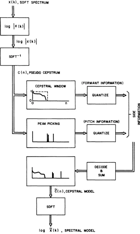
1.1 A Brief Description of the 32 band sub-band/transform coder algorithm

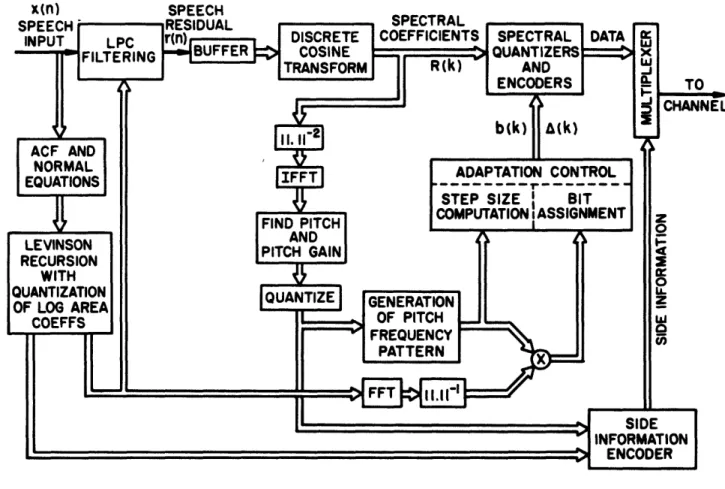
Fig. 1.2 is a block diagram for the basic 32 band sub-band/transform coder design that is studied in this thesis. The division of the voice signal into sub-bands is achieved by a 32-channel quadrature mirror filter (QMF) bank [13-161 which is described in Chapter Two. Each sub-band signal (represented in the figure as Yl through Y32) is independently coded and decoded using an APCM scheme incorporating a dynamically varying bit assignment and quantizer step size in each band. As in the case of transform coding, the bit assignment and quantizer step size vectors (represented in the figure as bi and AN respectively) for encoding

and decoding the sub-bands are provided by a spectral model of the incoming speech.

A new spectral model utilizing recent concepts of vector quantizing [17,191 has been employed in the new coder designs for representing the time-varying spectral envelope of the speech signal at a modest cost in computational complexity. The input speech is represented by a all-pole spectral model that is dynamically selected from among a small collection of such

models. This concept has been referred to in the literature as a switched source of all-pole spectral models" [181. We have experimented with a set of spectral models ranging from 4 to

32 in number in which each model is represented by the LPC vector l/A,(z). Since each segment of incoming speech is quantized to one of a set of LPC vectors without explicitly performing a standard LPC analysis, the method can be though of as a technique for quantizing input LPC speech vectors. Each spectral model (defined in the figure by the codeword (C,),

which can be selected from the set, defines a one-to-one mapping to a bit assignment pattern in the bit assignment codebooks for encoding and decoding incoming speech. Generally speaking, the bit assignments have been computed so that the majority of the available bits are assigned to bands where the signal is estimated to be the strongest.

The best LPC model for each 16 msec segment of speech is selected from the collection of LPC vectors so as to minimize the log likelihood ratio distortion measure [22] between the

(n CHANNEL

r

Il· 10 -P_0" c-i_r\t En -;D YD

-speech and template spectra. This LPC model yields the minimum residual energy of the signals obtained from filtering the input speech segment with each inverse LPC filter A,(z). The square root of the minimum residual energy, XA, is the gain term of the best LPC

template (or model) [281 and is used with that template for setting the quantizer step sizes for encoding and decoding each band.

Since the number of LPC template vectors used to represent the input speech is very small, if the vectors are reasonably chosen, the spectral distances between any two of these vectors will necessarily be large' in order to encompass a variety of speech sounds. This has been an important consideration for developing a simple and efficient method for selecting the minimum energy residual necessary for the template codeword and gain selection. The lower left hand corner of Fig. 1.2 depicts such a method. The square root of the Nth residual energy,

\/a, is estimated by low-pass filtering the absolute value of the Nth residual signal. This

signal is obtained from filtering a speech segment with the Nth inverse template filter AN(z).

These computations are executed for each of the N inverse template filters for each segment of speech. The best template is selected to have the minimum gain estimate

i/.

The LPC spectral templates are generated with the aid of a clustering method previously applied to speech recognition [24,25] and vector quantizing for LPC vocoders [17-19]. The procedure identifies a set of LPC template vectors as cluster centers such that the average (log likelihood ratio) spectral distortion measure from all input vectors to their best match in the template vector collection is minimized [19,20].

In order that the speech coder be speaker independent, the clustering program inputs a large set of autocorrelation training vectors derived (based on a frame by frame analysis) from a speech database including a wide variety of talkers. The majority of the silence (background noise) must be eliminated from this database to ensure that numerous shades of background noise are not represented by the input training vectors.

sub-band coding and transform coding techniques. The structure accomplishes a 32-sub-band decomposition of speech in which the bit assignment patterns and step sizes for encoding and decoding each sub-band are dynamically updated on the basis of a new spectral model. This model is based on recent concepts of vector quantizing in conjunction with known clustering methods. Since the new spectral model is much simpler and requires less side information* than recent spectral models that have been applied to ATC algorithms (such as models based on homomorphic analysis [3] and standard LPC analysis [341), the approach taken in Fig. 1.2 appears inviting.

1.2 The Scope of the Thesis

This thesis reports on the study of two new techniques for 32 band sub-band/transform coding at 16 kb/s rates. Both coders have been implemented and tested on a general purpose digital computer. The proposed coding schemes offer good quality reconstructed speech at complexities that occupy the middle range between simpler sub-band and more complex adaptive transform coding techniques. Recent concepts of vector quantizing in conjunction with clustering methods have been employed for modeling speech with a switched source of all-pole spectral templates for dynamic bit assignments and adaptive quantization. An important objective of this thesis is to gain insight into the performance - complexity tradeoffs involved in these middle range schemes. The thesis is structured so that the fundamental components of the algorithm in Fig. 1.2 are separately discussed, prior to presenting a review of our findings in Chapters 5 and 6. The thesis is organized as follows:

Chapter 2 describes a 32-band quadrature mirror filter bank implemented with a parallel structure (utilizing a technique proposed by Esteban and Galand [14]) for sub-band decomposition of the speech signal. A derivation of the structure is given along with a discussion of its implementation and performance.

* side information is information that is separately transmitted across the channel to establish the bit assigmets and quantizer step sizes for the decoder. This corresponds to the 'codeword' and 'gain' of Fig. 1.2.

Chapter 3 is concerned with the spectral side information model for the speech signal. The chapter begins by describing how the spectral templates were derived from a training speech data base and is followed by a discussion of the model for template picking and gain computation. The chapter concludes with an evaluation of the tradeoff between the accuracy and complexity of the template model for various LPC orders and numbers of templates.

Chapter 4 presents the bit assignment algorithm used for generating the bit assignment codebooks. Bit assignment methods for a flat noise spectrum as well as spectral shaping of the quantization noise are discussed.

Chapter 5 is concerned with adaptive quantization of narrow band signals for coding the 32 sub-bands. The chapter begins with an overview of adaptive quantization techniques that have been applied to sub-band and transform coding. Two techniques for quantizer step-size adaptation corresponding to both coders are developed and discussed.

Chapter 6 presents the results of an informal comparison test for quality which was performed in order to compare the effectiveness of the coder designs presented in Chapter with simpler sub-band and more complex transform coding methods. The overall performance/complexity trade-offs of the 32 band coders are evaluated relative to these methods.

Chapter 7 concludes the thesis with a summary of major results and some suggestions for further research.

CHAPTER II

2. A 32-BAND QUADRATURE MIRROR FILTER BANK IMPLEMENTED WITH A

PARALLEL STRUCTURE 2.1 Introduction

Since the design of efficient filter bank techniques in the midrange of 16 to 64 bands has not been well established, we have utilized concepts of quadrature mirror filters based on earlier sub-band work. This design has provided a good filter-bank analysis and synthesis framework for algorithm study in spite of its large storage and processing requirements for a 32 band design.

Sub-band decomposition based on a tree arrangement of quadrature mirror filters (QMF's) has been applied at low bit rates, and has been shown to avoid aliasing effects due to finite filter transition bandwidths and decimation [13]. The filter bank described in this chapter was derived from a 5 level tree structure QMF bank utilizing a technique proposed by Esteban and Galand [14]. Although it is strictly equivalent to the tree approach, the parallel approach

allowed additional implementation simplicity although extra coefficient storage is necessary. 2.2 Principles of Tree Decomposition

Fig. 2.1 shows the classical 2 band QMF filter bank for decomposition of the signal x(n) into 2 contiguous sub-bands. In this implementation x(t) is lowpass filtered to its Nyquist frequency Q,/2 then sampled at 0, yielding x(n). The signal x(n) is filtered by a lowpass filter HI(o), and a highpass filter H2(W). Since the spectra of xl(n) and x2(n) occupy only 1/2

the Nyquist bandwidth the sampling rate can be decimated by a factor of 2. This results in the signals y(n) and y2(n) obtained from decimating xl(n) and x2(n) respectively. In the

receiver the signals yl(n) and y2(n) are interpolated by a factor of 2 and filtered by K,(w) and

K2(w) respectively. These signals are then added to produce the reconstructed signal s(n).

ro (A 11-NU I .

r1

U Ir cn

3

K

r

I-0 D 'H I--_H -(D 0 o Ct rU cr I

vlC

c-H ct)i e,

Fig. 2.1 will result in aliasing terms. It has been demonstrated [131 that these terms are cancelled by choosing HI(o), K1(w), H2(o), K2(o) such that the following conditions hold:

1. H(w) is a symmetrical FIR filter of even order N. 2. H2() - H=(w+w).

3. K,(o)

Hl(o).

4. IH,(w,)12+ IHI(+,r)2,

5. K2(co) - H2(W).

In this case s(n) - x(n-N+1). That is, the output signal is a replica of the input signal (neglecting the gain factor of 1/2) with an N - 1 sample delay. A derivation of this result and the above five conditions is presented in Appendix I.

This decomposition can be extended to more than two sub-bands by highpass and lowpass filtering the signals yl(n) and y2(n) and reducing the sampling rate accordingly. In the general case the input signal, x(n), is split into 2 sub-band signals sampled at ,/2M by a M-stage tree arrangement of decimated filters. The sub-band signals are reconstructed to form the output by a symmetric tree arrangement of interpolation filters. Fig. 2.2 shows this for M - 5. 2.3 Derivation of the Parallel Structure From the Tree Structure

Fig. 2.3 depicts the parallel structure implemented for decomposition of the signal x(n) into 32 contiguous sub-bands. This is achieved by filtering with a bank of 32 contiguous bandpass filters Fi(z) uniformly covering the frequency range 0 S w r. Since the resulting spectra

X(w,) occupy only 1/32 of the Nyquist bandwidth, the sampling rate is then decimated by a

factor of 32 to yield the signals y(n). These signals occupy the full Nyquist bandwidth as a result of the frequency domain translation and stretching operations achieved by decimation. The reconstructed signal s(n) is obtained by interpolating the signals yl(n) by a factor of 32, then by re-filtering and summing the outputs.

vq H

.I

C7

., ro

It N Nl _I

_'

IV I_ _'II : I I IN It N _i IWI a a i i i , I l ' i , ,I I 4I I I I I"I- W '5 -7I 1S I II Ii'

..-- I- -- - - o -- -- I a

I I I

P. ., H- < ct (D ct-m U (D 3C CD AD 0 ct-(D 0 I I I

x W

I"

x N S to

1~~~~~~~~~~~~~~~~~~~~~~~~~~~2

Nr X X Xt I l> thi t I I I I I II I I I I I I I I I I I I I I

I

I

III

A ) v, Hd P ' P F- 0'q (

L

', L _I

7

L-'-B n '"~1 r 1 F1 r,--1 _ _ It

-We can derive a set of 32 conditions which are necessary to insure the perfect reconstruction of s (n) (without aliasing). The z-transforms of xi (n) are given by

X,(z) - F,(z)X(z) .

(2.1)

The z transforms of the decimated signals y,(n) are [11

32-1e-

_j

1/32)

Y

(Z)

-I

X(e

z (2.2)

Interpolating 2.2 results in

U,(z)

_ Y(z 32). (2.3)

Final filtering results in

Tf(z) = G,(z)U,(z) , (2.4)

32

S(z)

T(z).

(2.5)

i-l

Combining equations (2.1) through (2.5) yields

1 32 31 2t

3S

2

-

Gi(z)

F

,(e

32

z)X(e

l

32 z)

(2.6)

Elimination of the aliasing terms in (2.6) requires that

S()-

32

X(z) ,(z)F(z), (2.7)

32 _j 2 r

G,(z)Fg(e 32 z)O, I

Q

31. (2.8)

i-I

By identifying the z-transforms of the sub-band signals for the parallel and tree structures it is possible to determine the relationship between the coefficients of both structures.

For the parallel implementation, the first sub-band signal yl(n) is given from Eqs. (2.1) and (2.2) by

31 2! 2.

Yl(z)

-

F(e1 32 132) 32 z/32) (2.9)

-0

Referring to figure (2.2) we can derive the expression for the first sub-band signal of the tree structure

Al(z)

IX(z")H(zs

)

+ X(--z)HI(-ZA)]

(2.10a)

A2(z) =-i-

IA

(zA)H2(z) + A (-zA)H 2(--z)l (2. 10b)

A3(z) 2 [A2(z')H' 3(z) + A2(-Z%)H3(-z'A)] (2.10c)

A4(Z) -= [43(ZH)H4(z) + A3(-Z')H 4(-z')] (2. 10d)

Yl(Z)

-

'

[A4

(zA)Hs(zA) + A4(-z')Hs(-z)]

(2.10e)

Equating equations 2.9 and 2.10e gives

F.(z)

-

H l(z )H

₂

(z

2

)H

₃

(Z4)H

₄

(z)H (Z

16)

with repetition of the pattern in other bands. A complete listing for all the analysis filters Ft (z) is given in Table I of Appendix I.

The synthesis filters Gi(z) can be obtained by an analogous procedure. For the signal tl(n) of Fig. 2.3 we can write

T1(z) Y 323(z)G1(z) . (2.11)

Referring to figure 2.2 we can write

B4(z)- Y!(z2)Hs(z) , (2.12a)

B

3

(z) - B4(z

2

)H(z) ,

(2.12b)

B2(z) B3(z2)H3(z) , (2.12c)

Bl(z)

B

2

(z

2

)H

2

(z)) ,

(2.12d)

Tl(z)

Bl(z

2

)Hl(z) .

(2.12e)

G (z) - F

1

(z).

It is shown more generally that

OG (z) - (-l)'-)F,(z). (2.13)

The equations for the analysis (and hence the synthesis) filters in Table I of Appendix I suggest a straightforward filter implementation procedure. Consider for example the implementation of the fourth analysis filter described by the z-transform

F

4

(z) - H l(z )H

2

(z

2

)H

3

(z

4

)H4(-z')Hs(z

16

) .

(2.14a)

The corresponding impulse response can be expressed as

f4(n) -

h(n)*h(

2( )2(n )*h 3()(n) (2.14b)

*(-1)

8h4(

n ),s(n)*hs(

16(n)

where the sequence WL (n) is defined to be nonzero only at integer multiples of L: that is

L(n) l, n -O0, L, 2L,...

=

0,

otherwise .

Equation (2.14b) is the result of first forming the sequences h (n), h2(n), h3(n), (-l)"h 4(n),

and hs(n), then interpolating these sequences by factors of 1, 2, 4, 8, and 16, respectively; and convolving the results to obtain f 4(n).

2.4 The Implementation

Examination of the z-transforms of the filters in Table 1 of Appendix I reveal symmetries which can be exploited to minimize coefficient storage space. By noting that

F(z)

-

F

32

(-z), F

2

(z) - F

31

(-z),

..

.

F

6

(z) - F1

7

(-z)

it is seen that the upper 16 filters can be obtained from the lower 16 filters by a shift of radians which amounts to alternating the sign of every other filter coefficient in the time domain. Furthermore it can be seen that the odd numbered filters Fl(z),F 3(z), are all

symmetric, and the even numbered filters F2(z),F4(z) .'''.. are all anti-symmetric. A direct

first half of the first (or last) 16 filters.

The actual quadrature mirror filters used for this implementation were designed by J. D. Johnston using the Hooke and Jeaves optimization algorithm [161; 64 tap, 32 tap, 24 tap, 16 tap, and 12 tap filters were used in the first, second, third, fourth and fifth splits respectively. A list of coefficients for these five filters (h I(n), h2(n), h3(n), hA(n), hs(n)) is given in Table

2 of Appendix I together with plots of frequency response and QMF ripple. Figure I.I (of Appendix I) depicts the magnitude response of the 32 bandpass filters F(z) through F32(z)

which were designed using the above five filters.

The filter bank was implemented in computer simulation on a general purpose computer, a Data General AP130, using an array processor. The analysis, filtering, and decimation operations of figure 2.3 was achieved using a direct form structure of an M to 1 decimation

[12]. Interpolation operations and synthesis filtering were achieved using a standard polyphase filter structure [12].

2.5 Filter Bank Transfer Function

It is possible to derive an expression for the transfer function of the analysis/synthesis filter bank of figure 2.3, which can be interpreted in terms of a magnitude ripple in the frequency domain. By substitution of Eq. (2.13) into (2.7) we obtain

1

S(z)

X(z)

f(z)(-)(-)F(z)

.

(2.15)

Re-arranging terms gives

S(z) = j32IX(z) {F2 (Z)-F2 (z)] + [-F22

(z)+F32,

(z)J +

(2.iSa)

[F2(z)-F2(z)]

+

...

[-F26 ()+F2 ()]

+

Since F32(z)-FI(-z), F2(z)-F 31(-z) F30(z)-F 3(-z),... F1 6(z)Fl 7(-z), (2.15a) becomes a

S(z) 31 X(z){[F(z)-F (z)1 +

[F

(z)-F3 (-z) +

(2.15b)

[F2(z)-F2(-z)] +.

+[

()-F2(-z)].

S(z) can be expressed more compactly by summing over odd terms as

1 31

X(z)

I

[F2(z)-F2(-)] (z).

(2.16)

32 oddJ-1

For F (z) a symmetric FIR filter of even order it can be shown that (see Eq. I.13b of Appendix

I)

L.

I[F,

2_{(z)- F,}2_{(-Z)] -}

_[IFi

("

_)l2

₊

_{IF,(w+r)2]c(NI}

"

_(2.17)

Evaluating (2.16) on the unit circle yields

S()

= 3X(Z)

I2 [IF(,)I2

+

IFI(c+W)I2]eJ1

i.

(2.18)

2 oddi-1

Since

F2(,) = F3 1(W+W), F4(w) - F29(w+r), F6(,) F27(O+Wr),

the Fourier transform of the output signal is given by

32 11

S (W)

312

X(a)e~j(N~I)"z Is(W) 12 (2.19)

Ignoring the gain term and the delay of N - 1 samples, perfect reconstruction of the input signal requires that

Z

IF(ci)

1

2

_in

_1.

_(2.20)

I-1

This term is plotted in figure 1.2 of Appendix I on a magnified dB scale indicating a peak-to-peak ripple of less than 0.074 dB.

2.6 Observations

The plot of Fig. I.1 confirms the performance of the filter bank design of this chapter for limiting the amount of internal aliasing between the bands of the analysis filters (the worst case is down 15 dB). The internal aliasing cancellation properties of the design is evidenced by the

'flat' frequency response shown in Fig. 1.2. Time domain testing has confirmed also that the filter bank is linear and shift invariant within practical limits. It is worth pointing out that because of the good frequency resolution of the analysis and synthesis filters their impulse responses are long in time (514 samples). The interpretation of these observations are postponed until Chapter 5.

CHAPTER III

3. A SPECTRAL SIDE INFORMATION MODEL FOR SPEECH SIGNALS 3.1 Introduction

A switched source of all-pole spectral templates is used for modeling incoming speech in order to achieve efficient dynamic bit assignment and quantizer step size adaptation for encoding the sub-band signals. These templates (which are represented as LPC vectors) are derived through an iterative process called a clustering algorithm which involves spectral comparisons on a large set of LPC training vectors derived by autocorrelation analysis on a speech database [24,25]. Once the templates comprising the vector codebook have been derived, it is necessary to dynamically select that template which best models the incoming speech.

The beginning of this chapter discusses the speech database and clustering algorithm for template generation. This is followed by the template selection scheme and an analysis of the tradeoffs between the accuracy and complexity of the spectral template model.

3.2 Derivation of the Spectral Templates

In order to generate a set of spectral templates, a training database was first established. The database was comprised of speech by 7 speakers, 4 male and 3 female. Each speaker contributed about 19.6 seconds of speech by uttering the same 10 phonetically balanced sentences. This resulted in a 137 second database. Forty-two seconds of silence was eliminated from this database to ensure that numerous shades of background noise did not occupy valuable space as spectral models.

The speech used was high quality microphone speech bandpassed from 100 Hz to 3500 Hz, sampled at 8 kHz, and quantized to 16 bits/sample. An LPC analysis using the autocorrelation method [28] was then performed on the data using an analysis window (Hamming window) of

length 256 samples (or 32 ms).* This window was shifted by 256 samples at a time generating about 3,000 vectors. Each vector was stored as a gain-normalized autocorrelation sequence,

[R,(n)/aM, n - 0,1,2,...,M), where M is the order of the LPC analysis and a is the

residual energy resulting from passing the windowed input segment through its corresponding LPC inverse filter.

This analysis was performed for LPC orders of 10,8,6,4 and 2 for 1,2,3,4, and 5 bit template codebooks** in order to select the LPC order and number of templates resulting in the best tradeoff between spectral modeling and the amount of "side information" required. As an example, figure II.1 of Appendix II shows frequency domain plots for 1,2,3,4 and 5 bit template codebooks derived from a fourth order LPC' analysis.

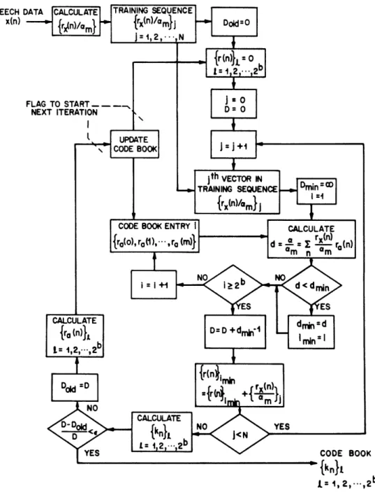
3.2.1 The clustering algorithm for generating the templates

The clustering algorithm used to generate spectral templates was developed by B. H. Juang [19] and implemented by L. R. Rabiner [20]. These templates were selected such that an average spectral distortion measure - in this case the log likelihood ratio [22,231 - from all input vectors to their best match in the template vector collection was minimized [17,19]. A number of spectral distortion measures have been discussed by Gray and Markel [21] and Gray et al. [23]. In theory, any of these distortion measures can be used in the clustering algorithm. However, for LPC vector quantizing, the distortion measure should be consistent with the residual energy minimization concept of the LPC analysis process [19]. Three distortion measures have been found with this property [23]: the Itakura-Saito measure, the Itakura measure, and the likelihood ratio measure. Because of practical considerations such as computation, storage complexity and variations in the input gain level, the likelihood ratio measure has been found to be more appropriate for LPC vector quantization [19].

* This is a standard size analysis window for speech [28]. * A b bit template codebook contains 2b templates.

Briefly, the procedure taken by the clustering algorithm was as follows [19]. I. Start at 1 bit with 2 initial codewords.

2. For each gain normalized autocorrelation vector in the training database, perform an exhaustive search over all available codewords to find its nearest neighbor (using the log-likelihood spectral distance measure) and then assign the input to the corresponding cell. 3. Update each cells centroid by solving the LPC equation corresponding to the average

autocorrelation sequence and use the new centroids as the current codewords.

4. Repeat steps 2) and 3) until the change in average distortion drops below a preset threshold.

5. If the maximum desired number of bits is reached, stop the process; if not, proceed to 6).

6. Initialize codewords for the next bit stage by perturbing each centroid. A flowchart of this procedure is given in figure 3.1 [19].

3.3 A Dynamic Template Selection Scheme

Once the LPC order and. the number of templates comprising the vector codebook have been selected, it is necessary to dynamically select that template which best models each incoming speech frame of 4 ms (32 samples). This template is chosen to minimize the log likelihood ratio distance measure between the best (gain-normalized) LPC model of the speech spectra, and the template spectra. This measure compares two gain-normalized model spectra giving the best spectral match possible over all gain values [21].

Let X(z) be the z-transform of a frame of speech and let VcjM/AM(z) be the optimal Mth-order LPC model of X(z). The squared gain term aM is the residual energy resulting from inverse filtering X(z) with AM (z). Also, let 1/Ai(z) be any Mth order, gain-normalized all-pole filter from the vector codebook. Inverse filtering X(z) with A:(z) results in a residual

ai, a a. al is given as:

i

21 il

(w),(o

)rd

(3.1)

The Log-Likelihood Ratio measure between the optimum (gain normalized) LPC model of the speech spectra l/AM(z), and the template spectra l/A:(z) is defined as [17,19,22]:

dLR log log 2 IA 2 d,. (3.2)

SPEECH x(n)

K

tKnjtl

j= 1, 2, ..,2b

Fig. 3.1 Flowchart of codebook generation

procedure. Juang et al.: Distortion

Clearly, minimizing dLR is equivalent to minimizing the residual energy ai since the optimal (minimum) aM is fixed for a given input frame.

Figure 1.2 illustrates a scheme for computing /T/A(z), the best template model of the speech - represented by the gain X'7 and the template number (or bit assignment index) Ci. According to this scheme the input speech s(n) is processed frame by frame to result in a template selection and gain computation every 16 ms. Since speech is approximately stationary over 16 mS intervals, the bit assignment pattern and quantizer step sizes for coding the sub-band signals need only be updated every four, 4 ms frames, hence the side information

(consisting of the gain and bit assignment index) need only be transmitted every 4 frames. In principle the optimum spectral template for modeling a particular frame of speech should be chosen such that the residual energy resulting from inverse filtering a windowed speech segment of s(n) with the inverse FIR filter A (z) is minimized. The windowed speech segment corresponding to the Q-th (32 sample) frame can be conveniently expressed as

sq(n) = s(n +32Q) w(n) (3.3)

where (n) is a finite length window (e.g. a Hamming window) that is identically zero outside the interval 0 n < N - 1. The residual energy oi which results from inverse filtering Sq(z)

with Ai(z) can be expressed in the time domain as:

I+~ co2 N-I+M

where e(n) -= S(n) * ai(n) and M is the LPC order of the templates. The minimum residual

a, is the squared gain estimate for the template model.

We have mentioned in the first chapter that by employing a small number of LPC templates in the vector codebook we are doing a "course" spectral modeling of the input speech. Although the scheme of figure 1.2 for computing the best template model is not strictly equivalent to the method described above, its performance and computational efficiency for implementation on a digital signal processing chip justify its implementation. In this method

the input signal s(n) is not windowed. The spectral template is chosen by minimizing an estimate for Va/7, the square root of the residual energy. This minimum estimate has been found to be proportional to the gain of the optimal template model. The absolute value of the residual signal

i(n)l

- Is(n) * at(n)l is LP filtered with a -pole HR filter with unit sample response

h(n) G(1-)0"

U

(n) (3.5)

to compute the estimate of i/a; where G, 0, and U are defined below. This estimate

s e

lfi(k)lh(n-k)

(3.6)

is evaluated for selecting the templatemplate and gain every 128 samples (16 ms).

An explanation of the parameters of the model is now given. G is the proportionality constant chosen to optimize the gain estimate. is selected to control the exponential time constant of the impulse response of h(n) and hence the number of samples of li(n)I which are averaged in Eq. (3.6) to form the gain estimate of X/. B is set to .98 corresponding to a

time constant of approximately 50 samples (6.25 ms). U is the unit step function.

3.4 An Evaluation of the Tradeoffs between the Spectral Accuracy and Complexity of the Template Model

The complexity of the spectral side information model developed in this chapter is proportional to the LPC order and the number of templates employed in the gain and template selection scheme of figure 1.2. Since the amount of processing required for template and gain picking (the number of multiplications and additions performed by the hardware for each template selection) varies proportionally with the complexity of the model, some tradeoffs need to be made between the accuracy in modeling the speech spectrum and the amount of processing required by the scheme in figure 1.2.

In order to select the LPC order and the number of templates for computation of the side information, an experimental relationship has been derived between the number of templates,

their LPC orders, and the spectral accuracy of the model. An evaluation of the spectral accuracy of the template model was based on spectral distance measurements (calculated every 4 ms frame) between the template spectral model and a standard 14th order LPC analysis spectrum of the input.

Both spectra were represented by 1024 point DFT's of gain normalized LPC spectra. A 256 point Hamming analysis window was shifted 32 samples at a time for computing the LPC spectrum of the input - the template model was the output of the template picking procedure discussed in the previous section.

Three spectral distance measures corresponding to the first, second, and fourth L norms were calculated in the log-domain (in bits) for every 4 mS frame of input speech. These distance measures are given for the pth norm as*

E,(n)

=

--

{0

2

A(k)

-log

2

I(k)} ]

(3.7)

where SA(k) and ST(k) are 1024 point DFT's of the gain normalized actual and template LPC spectra respectively. This error measure was calculated in the log2 domain because the bit

assignment in any band is proportional to the log magnitude of the optimum template in that band. Further details of this are considered in Chapter 4.

Each error measure E was averaged over time - using a speech file which contained no silence - to compute an average spectral error. This was done for various LPC orders and numbers of the templates.

The functional relationship discovered between the number of templates, their LPC orders, and the spectral accuracy of the model is plotted in figure 3.2 for p - 2.*

The subscript n is a reminder that the DFT's are functions of time as well as frequency.

0 The same plots for p - 4 and I show the same trends but assign greater and lesser emphasis, respectively, to the spectral peaks.

Ct

V Ct _(DX' fD CD-(1) O (D c (D CD 1 * O ct CD D H-I(D ct q,'1 CD (D -p~ · N a- t RMS ERROR IN BITS'

o0

0 o 0 0 0 o , _ b i O - 0 w O - N (A

I

I

li

I

I ~i I I 'I I

I

II '

t

tt

t

rI / , m 4 -4 U. cn (

These plots need some explaining. From an intuitive standpoint we expect that for a given number of templates the spectral error should decrease monotonically as the LPC order of the templates increase. This intuition is only correct if there are enough templates, or cluster centers, for the clustering algorithm to form sufficiently 'tight' clusters to properly model all the different speech sounds. Only with 32 templates (or more) do we observe monotonically decreasing spectral error with increasing LPC order. When fewer templates are used the spectral error increases when the LPC order exceeds 4.

Figure 3.3 shows an example of the accuracy of the template model for two complexity extremes. The figure shows log magnitude plots of an actual LPC spectrum (the dotted line) superimposed over the best template LPC spectrum (the solid line) for the case of a four template 2nd order LPC analysis (shown in Fig. 3.3a) and a 32 template 10th order LPC analysis (shown in figure 3.3b).

Eight, fourth order LPC templates were selected as a first cut tradeoff between the amount of processing and the accuracy of the resulting spectral model. This choice results in approximately 40 multiplies and adds (in the implementation of Fig. 1.2) which are required per frame for selection of the template and gain term, and an average RMS error in bits of less than one.

3.4.1 Observations

Tests have been performed over a wide range of complexities of the template side information model. These tests are in general agreement with the experimentally derived relationship between the LPC order of the templates, the number of templates, and the accuracy of the model. For example, the four best sounding coding schemes were obtained using 32 spectral templates of 10th, 8th, 6th, and 4th order LPC with qualities from highest to lowest in this order. Listening tests later performed with side information complexities of up to 128 templates with 10th order LPC yielded only differential improvements in speech quality over the 32 template model.

LOG MAGNITUDE LOG MAGNITUDE

0

-1 e~D

ct

(D t I-o U} · I-Ct 0F '- co i-ctQ ct D t O . ctD (D o OC -CD O c-(D (D H- (D c o

o

c-CD O ct VI ' Cn F-a O D s

aoo

H (D

C(D

t

-(D 4 P1 ~1 m 0r

O

v

i-~ W

ct

3

30 HCD (D O PO I-ct Y-(D _I-S r1 pQ

p)o

Hj-Ci_H.

_ct

ccn v r I P) C--En P N I I-I O

It is worth pointing out that although the time averaged RMS spectral error in figure 3.2 ranges over only a quarter of one bit the corresponding audible range of coded speech quality varies quite vastly. In general, higher order L, norm error measures increase the error spread because they give more weight to the peak errors in the spectral model. Nevertheless, the error norm order must exceed 4 to get error spreads in excess of only three tenths of one bit.

4. A BIT ASSIGNMENT SCHEME FOR SPECTRAL NOISE SHAPING

4.1 Introduction

The bit assignment scheme determines the number of bits that are allocated for quantizing each sub-band signal of the QMF analysis filter bank. The algorithms presented in this chapter are used for off-line calculation of the bit assignment codebooks of Fig. 1.2. The bit assignment decision is based on a local estimate of the amplitude variance of the signal in each band as obtained from the spectral template used to represent the speech. The th sub-band is uniformly quantized with quantizer size Ai and 2 ' quantizer levels.

This chapter discusses a bit assignment technique for achieving a quantizing noise power which is flat in frequency, as well as a technique for achieving a noise power which follows" the spectral amplitude of the speech signal for auditory masking of the noise [2]. The techniques presented in this chapter are valid subject to the assumptions that:

1. The spectral side information model provides a good estimate of the amplitude variance of the sub-band signals.

2. The quantizer step sizes A are well adapted to the amplitude variance of the signal in each sub-band.

Under these assumptions the number of levels assigned for quantizing the sub-band signal in any channel will determine the 'coarseness' of the quantization in this channel, and hence the SNR obtained for quantizing that channel.

4.2 Bit Assignment for Fiat Noise Power

Let us assume that the sub-band output sequence yi (na) of the ith sub-band is a sequence of statistically independent, stationary, Gaussian random variables with zero mean and variance a2_{. The estimate of 2 is provided by the template estimate of the spectral magnitude in band}

i. If an average mean-squared quantization error D* is minimized, the optimal bit assignment for the ith sub-band signal is given by [29]

b - +

₂

log2 D*

_{, D*}

(4.1) The second term is the lower bound rate given by rate distortion theory for independent, Gaussian, r.v.'s with variance D* [1]. is a correction term that accounts for the performance of practical quantizers; it depends on the type of quantizer and the PDF of the signal to be quantized. The dependence of bi on will be neglected [29]. D, the average mean-squared

distortion or quantization noise variance is defined as

D*

32 2(i) (4.2)

where a,2(i) is the quantization noise variance as a result of quantizing the ith output y. The parameter D* of Eq. (4.1) must be chosen such that

32

B -Z

b,

. (4.3)

-1I

The sum of the bits available for quantizing each channel is equal to the total number of bits available for quantizing each (32 sample) frame. At a 16 kb/s coding rate there are 250 frames/second and hence B is roughly 64 (neglecting requirements for transmission of side information of gain and template number). It has been shown [291 that the above bit assignment rule leads to a flat noise distribution in frequency, i.e., er 2(i) - D* for all i.

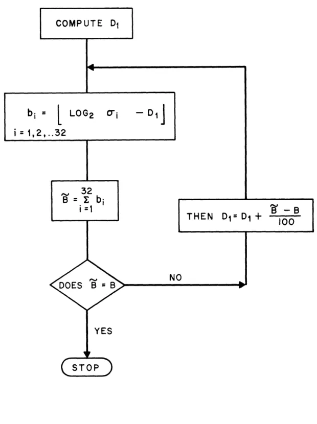
For practical implementation Eq. (4.1) can be modified as

b, i [log2(, - D (4.4)

where the operation J is defined as

0,

if u<0

uJ -

greatest

integer e u , if 0 e u < bMax (4.5)

bMAx if u ' bMAx

where bAx is the maximum number of bits allowed for quantizing any channel output, and D - log2D* (the quantization noise in bits). An algorithm for implementing the above bit

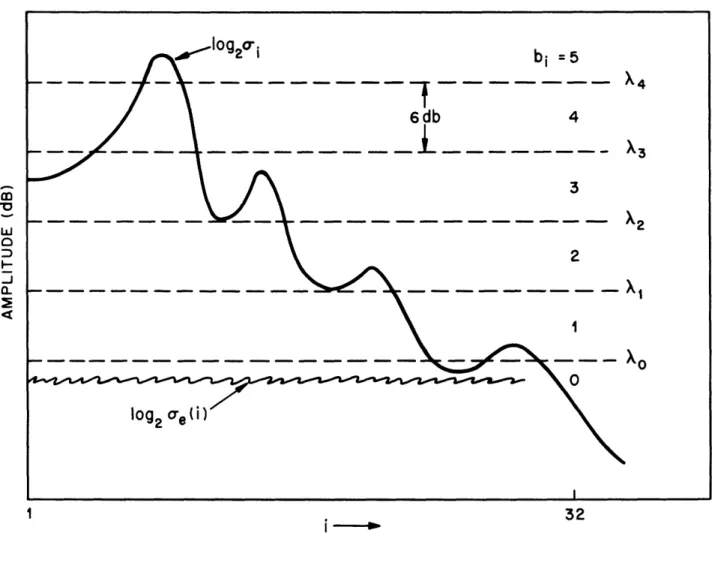
An intuitive explanation of why this bit assignment rule, based on a minimum mean-square error over the frame, leads to a fiat noise distribution in frequency can be seen in fig. 4.1 [2]. The horizontal dashed lines represent decision thresholds, Ai, for choosing the bit allocation bi. As an example, if the ith log spectral output log2a falls between A2 and A,, then 3 bits are

allocated for that coefficient. The thresholds are spaced 6 dB apart. Recall that for a uniform quantizer with proper loading the SNR is given by

SNR (dB) - 6B + [4.77 - 20 loglo (4.6)

where ax is the standard deviation (RMS level) of the signal, and XMAX- A 21 - the maximum quantizer level. Hence for every 6 dB that vo is increased, one more bit, or 6 dB of signal-to-noise-ratio is added to the quantizer. Thus, the noise power remains flat across the frequency bands. Exceptions to this occur when log2ei < o and when log2ai > X4. These

cases correspond to the minimum and maximum bit assignments of 0, and say, 5 bits respectively. If the total number of bit assigned in this way is less than B - the number of bits available for quantizing the frame - then the level of the thresholds , (proportional to

D*) are uniformly reduced. The threshold levels are uniformly increased if the total number of

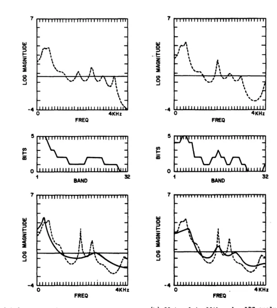
bits is greater than B. An example bit assignment using this scheme for B - 61 is illustrated in Fig. 4.2b by the solid line. The dashed line of Fig. 4.2a depicts the log magnitude of a 4th order LPC template (taken from an 8 template set) model of input speech log2 i- . The

corresponding amplitude scale in bits' is indicated on the figure. 4.3 Bit Assignment for Noise SLaping

We have noted that the previous bit assignment scheme minimizes the noise variance a,2(i) - D* and results in a flat noise power across the spectrum that is proportional to ,. It is known from perceptual criteria that minimum mean-square error or a flat noise distribution is sub-optimal for masking the quantization noise in each frequency band. The distribution of quantization noise across the frequency channels can be controlled by a modified bit assignment

Fig. 4.1 Bit assignment rule for a flat noise

Fig. 4.1 Bit assignment rule for a flat noise

spectrum.

Tribolet and Crochiere et al.: Frequency Domain

Coding Of Speech. a

w

_J Q 32

BITS SCALE

(1

LOG MAGNITUDE SCALE

I a w_CD

z

a7 N

0

C-o", v-U' (D r o ct r0

CD

(D C c-I-O , ct'_P)

Z

z

~~~~~~~~~~~~~~~~~~~~~~~~~~~~~~~~~~~~~~~~~~~~~~~~I

I O~~~~~~ I~~~ I I -_{_- I} I _/

-o

!o

- -91 /-I I I I I

-

I

- I -

I

- JI--

I

I - / -- I - !~ II-( N or

-rule [2]

I W 2

bi - + log2 ifV i -

1,2,...,32

(4.7)

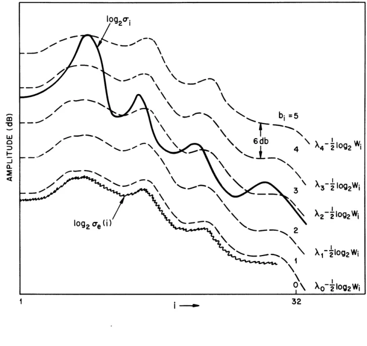
where W is a positive weighting function. This bit assignment minimizes the frequency weighted distortion measure

D*

32 Wga(i) 2 (4.8)

32

resulting in a noise variance given by

2(i) C

Wi

-

D*

i -1,...,32

(4.9)

where C is a constant. Figure 4.3 provides an interpretation of this frequency weighted bit assignment where the thresholds are now Xi -' log2Wi. Viewed another way we have

pre-emphasized a 2to W a2, and used the flat thresholds of figure 4.1.

The weighting function should be chosen in a manner in which the quantization noise is best masked by the speech signal [30]. The weighting function

WI - 2(r) (4.10)

belongs to a class of functions which provide a wide range of control over the shape of the quantizing noise relative to the shape of the speech spectrum by experimentally varying '. The case where y = 1 (uniform weighting) has already been discussed. This case yields a flat noise spectrum and the bit assignment obtained is such that the signal-to-noise-ratio has the shape of the spectrum. The case where y - 0 (inverse spectral weighting) leads to a flat bit assignment. Here the noise spectrum follows the input spectrum, and the signal-to-noise-ratio is constant as a function of frequency. The quantization noise distribution in bits' given approximately by

log102 o 109g2a -b, + 1 (4.11)

is depicted by the dashed lines in figures 4.4a and 4.4b for y - I and y - 0 respectively. In general, as the value of y is gradually varied between these two extremes (0<<1l), the noise spectrum will change from one that precisely follows the speech spectrum to a flat distribution.

c-cj

a.

X.

1 : _ 32

Fig. 4 .3

Frequency weighted bit assignment

rule.

Tribolet and rochiere et al.: Frequency Domain

Coding Of Speech.

LOG MAGNITUDE SCALE LOG MAGNITUDE SCALE V

0

I

r

C0 cn ) -01 0 I OC ii

Z

a

O1 BITS SCALE I -C

b

C-CD

z

3> H D O H-P ) H 'q09 cttO U) (D (D O CD -ctZ (D CD Ca H -) H'

o

DC

pJ a (DcS t CD c ctPc 0J O ) I I

I

I I I - I - I - I

-I

-I

I I (A

c

= I · ) BITS SCALE

In this chapter we have discussed a bit assignment scheme which enables us to experiment with bit assignment codebooks computed with an arbitrary amount of noise shaping - or control over the degree to which the spectral shape of the quantization noise follows the spectral envelope of the speech. Additional details of the bit assignment procedure are presented in Appendix III.