HAL Id: hal-03001127
https://hal.archives-ouvertes.fr/hal-03001127
Submitted on 18 Dec 2020
HAL is a multi-disciplinary open access
archive for the deposit and dissemination of
sci-entific research documents, whether they are
pub-lished or not. The documents may come from
teaching and research institutions in France or
abroad, or from public or private research centers.
L’archive ouverte pluridisciplinaire HAL, est
destinée au dépôt et à la diffusion de documents
scientifiques de niveau recherche, publiés ou non,
émanant des établissements d’enseignement et de
recherche français ou étrangers, des laboratoires
publics ou privés.
and surface melting in the Amundsen sector, West
Antarctica
Marion Donat-Magnin, Nicolas Jourdain, Hubert Gallée, Charles Amory,
Christoph Kittel, Xavier Fettweis, Jonathan Wille, Vincent Favier, Amine
Drira, Cécile Agosta
To cite this version:
Marion Donat-Magnin, Nicolas Jourdain, Hubert Gallée, Charles Amory, Christoph Kittel, et al..
Interannual variability of summer surface mass balance and surface melting in the Amundsen sector,
West Antarctica. The Cryosphere, Copernicus 2020, 14 (1), pp.229-249. �10.5194/tc-14-229-2020�.
�hal-03001127�
https://doi.org/10.5194/tc-14-229-2020
© Author(s) 2020. This work is distributed under the Creative Commons Attribution 4.0 License.
Interannual variability of summer surface mass balance and surface
melting in the Amundsen sector, West Antarctica
Marion Donat-Magnin1, Nicolas C. Jourdain1, Hubert Gallée1, Charles Amory3, Christoph Kittel3, Xavier Fettweis3, Jonathan D. Wille1, Vincent Favier1, Amine Drira1, and Cécile Agosta2
1Université Grenoble Alpes/CNRS/IRD/G-INP, IGE, 38000, Grenoble, France
2Laboratoire des Sciences du Climat et de l’Environnement, IPSL/CEA-CNRS-UVSQ UMR 8212, CEA Saclay,
91190, Gif-sur-Yvette, France
3F.R.S.-FNRS, Laboratory of Climatology, Department of Geography, University of Liège, 4000 Liège, Belgium
Correspondence: Marion Donat-Magnin (marion.donatmagnin@gmail.com) Received: 14 May 2019 – Discussion started: 24 May 2019
Revised: 29 November 2019 – Accepted: 12 December 2019 – Published: 27 January 2020
Abstract. Understanding the interannual variability of sur-face mass balance (SMB) and sursur-face melting in Antarc-tica is key to quantify the signal-to-noise ratio in climate trends, identify opportunities for multi-year climate predic-tions and assess the ability of climate models to respond to climate variability. Here we simulate summer SMB and sur-face melting from 1979 to 2017 using the Regional Atmo-sphere Model (MAR) at 10 km resolution over the drainage basins of the Amundsen Sea glaciers in West Antarctica. Our simulations reproduce the mean present-day climate in terms of near-surface temperature (mean overestimation of 0.10◦C), near-surface wind speed (mean underestimation of 0.42 m s−1), and SMB (relative bias < 20 % over Thwaites glacier). The simulated interannual variability of SMB and melting is also close to observation-based estimates.
For all the Amundsen glacial drainage basins, the in-terannual variability of summer SMB and surface melting is driven by two distinct mechanisms: high summer SMB tends to occur when the Amundsen Sea Low (ASL) is shifted southward and westward, while high summer melt rates tend to occur when ASL is shallower (i.e. anticyclonic anomaly). Both mechanisms create a northerly flow anomaly that increases moisture convergence and cloud cover over the Amundsen Sea and therefore favors snowfall and downward longwave radiation over the ice sheet. The part of interannual summer SMB variance explained by the ASL longitudinal migrations increases westward and reaches 40 % for Getz. Interannual variation in the ASL relative central pressure is the largest driver of melt rate variability, with 11 % to 21 % of
explained variance (increasing westward). While high sum-mer SMB and melt rates are both favored by positive phases of El Niño–Southern Oscillation (ENSO), the Southern Os-cillation Index (SOI) only explains 5 % to 16 % of SMB or melt rate interannual variance in our simulations, with mod-erate statistical significance. However, the part explained by SOI in the previous austral winter is greater, suggesting that at least a part of the ENSO–SMB and ENSO–melt relation-ships in summer is inherited from the previous austral winter. Possible mechanisms involve sea ice advection from the Ross Sea and intrusions of circumpolar deep water combined with melt-induced ocean overturning circulation in ice shelf cavi-ties. Finally, we do not find any correlation with the Southern Annular Mode (SAM) in summer.
1 Introduction
From 1992 to 2017, the Antarctic continent has contributed 7.6 ± 3.9 mm to the global mean sea level (Shepherd et al., 2018), and this contribution may increase over the next cen-tury (Ritz et al., 2015; DeConto and Pollard, 2016; Edwards et al., 2019). The recent mass loss from the Antarctic ice sheet is dominated by increased ice discharge into the ocean (Shepherd et al., 2018), but both surface mass balance (SMB) and ice discharge may significantly affect the Antarctic con-tribution to future sea level rise (Asay-Davis et al., 2017; Favier et al., 2017; Pattyn et al., 2018). Despite recent im-provements of ice sheet models motivated by newly available
satellite products over the last 10–20 years, large uncertain-ties remain in both the SMB and ice dynamics projections, hampering our ability to accurately predict future sea level rise (Favier et al., 2017; Shepherd and Nowicki, 2017).
The largest ice discharge changes in Antarctica are ob-served in the Amundsen sector with an increase of 77 % over the last decades (Mouginot et al., 2014). Current changes in the dynamics of glaciers flowing into the Amundsen Sea are dominated by ocean warming rather than changes in surface conditions over the ice sheet (Thoma et al., 2008; Pritchard et al., 2012; Turner et al., 2017; Jenkins et al., 2016, 2018). Increased oceanic melting can trigger marine ice sheet insta-bility, leading to increased ice discharge, thinning ice, and retreating grounding lines (Weertman, 1974; Schoof, 2007; Favier et al., 2014; Joughin et al., 2014). In parallel, in-creased surface air temperature can lead to surface melting, subsequent hydrofracturing and possibly major thinning and retreat of outlet glaciers after the collapse of ice shelves (De-Conto and Pollard, 2016). Surface melting, leading to melt-water ponding, drainage into crevasses and hydrofracturing, is thought to be the main cause of the Larsen ice shelf col-lapse over the last decades in the Antarctic Peninsula (van den Broeke, 2005; Scambos et al., 2009; Vaughan et al., 2003). While surface melting is currently limited to relatively rare events over the Amundsen Sea ice shelves (Nicolas and Bromwich, 2010; Trusel et al., 2012) and underlying reasons for melt pond formation versus active surface drainage net-work remain unclear (Bell et al., 2018), the rapid surface air warming observed (Steig et al., 2009; Bromwich et al., 2013) and projected (Bracegirdle et al., 2008) in this region suggests that surface melting could increase in the future. Our study focuses on the two atmospheric-related aspects that can significantly affect the contribution of the Amund-sen Sea sector to sea level rise, i.e., snowfall accumulation that is expected to increase in a warmer climate and therefore to reduce the mean sea level and surface melting that could potentially induce more ice discharge and therefore increase the mean sea level.
Understanding the interannual variability of SMB and sur-face melting is key to (i) quantify the signal-to-noise ra-tio in climate trends, (ii) identify opportunities for seasonal predictions and (iii) assess the capacity of climate models to respond to global climate variability. Furthermore, years with particularly strong surface (or oceanic) melting could trigger irreversible grounding line retreat without the need for a long-term climate trend. Interannual variability in the Amundsen Sea region is usually described in terms of con-nections with the El Niño–Southern Oscillation (ENSO), the Southern Annular Mode (SAM) and the Amundsen Sea Low (ASL). Our study revisits these connections through dedi-cated regional simulations based on the MAR model (Fet-tweis et al., 2017; Agosta et al., 2019). Hereafter, we start by reviewing recent literature on these climate connections.
The El Niño–Southern Oscillation (ENSO; Philander et al., 1989) is the leading mode of ocean and atmosphere
vari-ability in the tropical Pacific. It is the strongest climate fluc-tuation at the interannual timescale and can bring seasonal to multi-year climate predictability (e.g. Izumo et al., 2010). Global climate models predict an increasing number of ex-treme El Niño events in the future, with large global im-pacts (Cai et al., 2014, 2017). Interannual and decadal vari-ability in the tropical Pacific affects air temperature (Ding et al., 2011), snowfall (Bromwich et al., 2000; Cullather et al., 1996; Genthon and Cosme, 2003), sea ice extent (Pope et al., 2017; Raphael and Hobbs, 2014) and upwelling of circum-polar deep water favoring ice shelf basal melting (Dutrieux et al., 2014; Steig et al., 2012; Thoma et al., 2008) in West Antarctica. Recent studies found concurrences between El Niño events and summer surface melting over West Antarctic ice shelves (Deb et al., 2018; Nicolas et al., 2017; Scott et al., 2019). These connections are generally explained in terms of Rossby wave trains excited by tropical convection during El Niño events and inducing an anticyclonic anomaly over the Amundsen Sea (Ding et al., 2011). Paolo et al. (2018) re-ported a positive correlation between ENSO and the satellite-based ice shelf surface height in the Amundsen Sea over 1994–2017. Based on a detailed study of the extreme El Niño–La Niña sequence from 1997 to 1999, these authors suggested that El Niño events could increase snow accumula-tion but also increase ocean melting even more, thus leading to an overall ice shelf mass loss. The impact of ENSO was found to be stronger for the Dotson ice shelf and eastward and weaker for Pine Island and Thwaites (Paolo et al., 2018). However, the aforementioned studies were based on the anal-ysis of a few recent ENSO events and did not account for the highly variable properties of ENSO over multi-decadal peri-ods (e.g. Deser et al., 2012; Newman et al., 2011).
The Southern Annular Mode (SAM; Hartmann and Lo, 1998; Limpasuvan and Hartmann, 1999; Thompson and Wal-lace, 2000) is the dominant mode of atmospheric variability in the Southern Hemisphere and corresponds to a variation in the strength and position of the circumpolar westerlies. Over the last 3 to 5 decades, the SAM has exhibited a posi-tive trend; i.e., westerly winds have been strengthening and shifting poleward (Chen and Held, 2007; Jones et al., 2016; Marshall, 2003). Medley and Thomas (2019) found similar patterns for the SAM trends and the reconstructed snow ac-cumulation trend over 1801–2000. By contrast, the tempera-tures above the melting point over the Amundsen ice shelves were found to be largely insensitive to the polarity of the SAM (Deb et al., 2018). The SAM phase has also been sug-gested to influence the ENSO teleconnection to the south Pa-cific: in-phase ENSO and SAM events (i.e. El Niño–SAM− or La Niña–SAM+) favor anomalous transient eddy momen-tum fluxes in the Pacific that make the ENSO teleconnection to the South Pacific stronger than average (Fogt et al., 2011). The Amundsen Sea Low (ASL; Raphael et al., 2016; Turner et al., 2013a) is a dynamic low-pressure system lo-cated in the Pacific sector of the Southern Ocean and mov-ing across the Ross, Amundsen and Bellmov-ingshausen seas. The
ASL is important regionally and variations in its central pres-sure and position respectively reflect the second and third leading modes of the Southern Hemisphere climate (Scott et al., 2019, their Fig. 3). A westward shift of the ASL induces northerly flow anomalies over the Amundsen Sea, leading to warmer conditions and increased moisture transport over the ice sheet (Hosking et al., 2013, 2016; Thomas et al., 2015; Raphael et al., 2016; Fyke et al., 2017). Variations in the ASL central pressure also largely impact the West Antarc-tic climate: anAntarc-ticyclonic anomalies near 120◦W lead to ma-rine air intrusion over the ice sheet, thereby increasing cloud cover, longwave downward radiations and surface air tem-perature over the West Antarctic Ice Sheet (WAIS; Scott et al., 2019). While a deepening of the ASL is predicted for the twenty-first century in response to greenhouse gas emissions, its high regional variability makes future changes of the ASL difficult to predict (Hosking et al., 2016; Turner et al., 2009). Importantly, ENSO and SAM are not independent of each other, and both modes of climate variability impact the ASL (Fogt and Wovrosh, 2015). SAM influences the ASL cen-tral pressure since it affects the mean sea level pressure over Antarctica (Turner et al., 2013a). The second and third lead-ing modes of variability in the South Pacific have been sug-gested to be affected by Rossby wave trains induced by trop-ical convection anomalies (Mo and Higgins, 1998). In terms of ASL, it corresponds to a migration further west (east) dur-ing the La Niña (El Niño), but the difference has a low sta-tistical significance (Turner et al., 2013b). Scott et al. (2019) recently reported that El Niño conditions favored blocking in the Amundsen Sea as well as a negative SAM phase, both leading to warm surface air anomalies in West Antarctica.
In this study we revisit the influence of ENSO, SAM and ASL on summer SMB and melting over the drainage basins of the Amundsen sector in West Antarctica for the 1979– 2017 period. While the summer focus on melt rates is ob-vious, SMB in DJF (i.e. December–January–February) only represents 15 % of the annual SMB. It is nonetheless in-teresting to analyze the similarities and differences in what drives SMB and melting, and the modes of variability and their teleconnections to the Amundsen Sea region both have strong seasonal characteristics, so that each season needs to be considered separately. To do so, we simulate the sur-face conditions of the Amundsen Sea region over 1979– 2017 using the polar-adapted Regional Atmosphere Model (MAR) forced by the ERA-Interim reanalysis. Section 2 de-scribes the methodology followed in the study and presents the model and observations used for comparison. The model results are analyzed and evaluated against observations in Sect. 3. After evaluating the model skills (Sect. 3.1), we analyze and discuss our results on the potential impact of large-scale climate variabilities on the SMB and melting in Sects. 3.2 and 4. The conclusions are provided in Sect. 5.
2 Materials and method 2.1 Model
To estimate SMB and surface melt over the Amundsen sec-tor we use the Regional Atmosphere Model (MAR; Gallée and Schayes, 1994) and specifically version 3.9.3 (http://mar. cnrs.fr, last access: 25 September 2019). The model solves the primitive equations under the hydrostatic approximation. It solves conservation equations for specific humidity, cloud droplets, raindrops, cloud ice crystals and snow particles (Gallée, 1995; Gallée and Gorodetskaya, 2010). MAR repre-sents coupled interactions between the atmospheric surface boundary layer and the snowpack using the Soil Ice Snow Vegetation Atmosphere Transfer (SISVAT) originally devel-oped by De Ridder and Gallée (1998). The snow–ice part of SISVAT includes submodules for surface albedo, melt-water percolation, and refreezing and snow metamorphism based on an early version of the CROCUS model (Brun et al., 1992). MAR has been largely evaluated in polar regions (e.g. Amory et al., 2015; Gallée et al., 2015; Lang et al., 2015; Fettweis et al., 2017; Kittel et al., 2018; Agosta et al., 2019; Datta et al., 2019).
Our domain includes the drainage basins of the sen Sea Embayment glaciers and a large part of the Amund-sen Sea until 65◦S using oblique stereographic projection (EPSG: 3031). It covers an area of 2800 km × 2400 km at 10 km horizontal resolution (Fig. 1) and 24 vertical sigma levels located from approximately 1 to 15500 m above the ground. We use 30 snow layers, resolving the first 20 m of the snowpack, with a fine vertical resolution at the surface (1 mm) increasing with depth; snow layer thickness varies dynamically depending on the physical properties of overly-ing snow layer properties. If neighboroverly-ing layers have simi-lar properties, then layers are associated together. The radia-tive scheme and cloud properties are the same as in Datta et al. (2019) and the surface scheme including snow den-sity and roughness is the same as in Agosta et al. (2019). The model is forced, over the period 1979–2017, by ERA-Interim reanalysis (Dee et al., 2011), which performs well over Antarctica (Bromwich et al., 2011; Huai et al., 2019), at 6-hourly temporal resolution and relaxed over ∼ 50 km later-ally (pressure, wind, temperature, specific humidity; the re-laxation zone is shown in Fig. 1), at the top (i.e. above 10 km) of the troposphere (temperature, wind) and at the surface (sea ice concentration, sea surface temperature). The Bedmap2 surface elevation dataset is used for the ice sheet topography (Fretwell et al., 2013). The snowpack density and tempera-ture are initialized from the pan-Antarctic simulation from Agosta et al. (2019). Drifting snow is relatively infrequent in the Amundsen region (Lenaerts et al., 2012) so that the drift-ing snow module has been switched off in our configuration, similar to in Agosta et al. (2019).
In Sect. 3.2 we provide the SMB constituents averaged over individual drainage basins.
2.2 Antarctic surface observations
We make use of meteorological data from the SCAR database including observations from the Italian Antarctic Research Program (http://www.climantartide.it, last access: 25 September 2019), the Antarctic Meteorological Research Center (AMRC program) (http://amrc.ssec.wisc.edu/, last ac-cess: 25 September 2019) and the Australian Antarctic auto-matic weather station (AWS) dataset (http://aws.acecrc.org. au/, last access: 25 September 2019). Among the 243 AWSs available over Antarctica since 1980, we selected the 41 sta-tions (see Table S1 in the Supplement for station names) located no more than 15 km from the closest continental MAR grid point (even if the domain resolution is 10 km, sta-tions over islands or capes that are not resolved can be lo-cated farther than 15 km from the closest continental MAR grid point). For each location, modeled values (surface pres-sure, near-surface temperature and near-surface wind speed) are computed as the average-distance-weighted value of the four nearest continental grid points. A second selection crite-rion is also applied in order to reduce comparison errors due to the difference between the model surface elevation and the actual AWS elevation: we only retain observations with an el-evation difference lower than 250 m. This two-stage selection leaves 41 suitable AWSs in our domain (Fig. 1).
To evaluate the simulated SMB, we use airborne-radar data from Medley et al. (2013, 2014) covering the period 1980–2011. These data were collected through NASA’s Op-eration IceBridge campaign over the Thwaites and Pine Is-land basins. They are based on the CReSIS radar (Center for Remote Sensing of Ice Sheets), which is an ultra-wideband radar system able to measure the stratigraphy of the upper 20–30 m of the snowpack with a few centimeters in vertical resolution. Airborne-radar data were verified with 190 firn core accumulation records. To evaluate the SMB regional pattern at a broader scale, we also compared the simulated SMB with the observations gathered in the GLACIOCLIM-SAMBA dataset thoroughly described by Favier et al. (2013) and updated by Wang et al. (2016) that are covered by our do-main. Similar to Kittel et al. (2018) and Agosta et al. (2019), we selected the observations for which the measurement pe-riod extends from 1950 to 2018. Observations before 1979 (i.e., the beginning of our study period) were compared to the average SMB simulated by MAR provided they cover a period of at least 5 years, while observations after 1979 were compared to the SMB modeled by MAR for the observa-tion period. We then compared the modeled SMB computed by using a four-nearest inverse-distance-weighted method for each of the 124 selected SMB observations.
To evaluate simulated surface melt, we use satellite-derived estimates of surface meltwater production over 1999–2009 from Trusel et al. (2013), provided at 4.45 km resolution, and based on the QuickSCAT backscatter and calibrated with in situ observations. We also use data from Nicolas et al. (2017), who provide the number of melt
days at 25 km resolution over Antarctica. This product is based on passive microwave observations from the Scanning Microwave Multichannel Radiometer (SMMR), the Special Sensor Microwave/Imager (SSM/I) and the Special Sen-sor Microwave Imager/Sounder (SSMIS) spaceborne sen-sors and covers the 1978–2017 period. For a given grid cell and a given day, melt is assumed to occur as soon as one of the two daily observations of brightness tempera-ture exceeds a threshold value. As the identification of melt days may be sensitive to the algorithm, we also use the dataset from Picard et al. (2007), extended to 2018 (http:// pp.ige-grenoble.fr/pageperso/picardgh/melting/, last access: 25 September 2019). This dataset is also based on SMMR and SSM/I but uses the algorithms from Torinesi et al. (2003) and Picard and Fily (2006) to retrieve melt days. It is pro-vided as daily melt status at 25 km resolution over the Antarctic continent from 1979 to 2018.
2.3 Climate indices
To describe the ENSO, we use the Southern Oscillation Index (SOI) from the Global Climate Observing System (GCOS) Working Group on Surface Pressure (Ropelewski and Jones, 1987; https://www.esrl.noaa.gov/psd/gcos_wgsp/ Timeseries/SOI/, last access: 25 September 2019). The SOI corresponds to the normalized pressure difference between Tahiti and Darwin based on observations. The Rossby wave trains connecting the equatorial Pacific to Antarctica are ex-pected to develop within a few weeks in response to ENSO anomalies (e.g. Hoskins and Karoly, 1981; Mo and Higgins, 1998; Peters and Vargin, 2015), so we first use the syn-chronous (DJF) SOI in Sect. 3. The lagged relationship to ENSO is discussed in Sect. 4, where we use other 3-month averages of SOI such as JJA (June–July–August). SOI is pre-ferred to NINO3.4 because it gives slightly stronger correla-tions with the variability in the Amundsen Sea region (as also found by Scott et al., 2019; Holland et al., 2019), but very similar results were obtained using NINO3.4 (not shown).
We use the SAM index from NOAA/CPC (https: //stateoftheocean.osmc.noaa.gov/atm/sam.php, last access: 25 September 2019) to describe the primary mode of at-mospheric variability in the Southern Ocean (e.g., Marshall, 2003). The SAM index is calculated as the difference of mean zonal pressure between the latitudes of 40 and 65◦S based on NCEP/NCAR reanalysis which produces a SAM that is consistent with other reanalyses after 1979 (Ger-ber and Martineau, 2018). In the negative (positive) phase, the mean sea level pressure anomaly between the Antarc-tic and midlatitudes is positive (negative) and leads to a weaker (stronger) polar jet. Thus, positive (negative) values of the SAM index correspond to westerlies that are stronger (weaker) than average over the middle to high latitudes (50– 70◦S) and weaker (stronger) westerlies in the midlatitudes (30–50◦S).
We use two other indices to describe the evolution of the migration and intensity variations in the Amund-sen Sea Low (ASL). The datasets are provided by the British Antarctic Survey (https://legacy.bas.ac.uk/ data/absl/ASL-index-Version2-Seasonal-ERA-Interim_ Hosking2016.txt, last access: 25 September 2019) and calculated from the ERA-Interim reanalysis. To describe the migration, we use the longitudinal position of the ASL defined as the position of the minimum pressure within the box 80–60◦S, 170–298◦E (Hosking et al., 2016), defined in degrees east. A decrease in the longitudinal position index hence corresponds to a westward shift of the ASL. To describe the intensity of the ASL, we use the relative central pressure of the ASL calculated as the minimum pressure in the aforementioned box minus the average pressure over that box (Hosking et al., 2016). A more intense ASL (deeper depression) is therefore represented by a lower index.
The SAM and ASL indices are defined regionally, and we do not expect any lag with summer SMB, so these indices are therefore calculated as DJF averages. All the correlations are calculated using detrended time series.
The correlations between these four indices are indicated in Table 1. A significant anticorrelation is obtained between the SAM index and ENSO (i.e. −SOI) as previously reported by Fogt et al. (2011). There is no significant relationship be-tween the ASL longitudinal position and ENSO or SAM, as previously reported by Turner et al. (2013a). The relative central pressure also varies independently from SAM, ENSO and the ASL longitudinal position. Numerous previous stud-ies used the absolute rather than relative central pressure to characterize the ASL, but this index is strongly correlated to the SAM index and cannot be considered independently (Table 1). As proposed by Hosking et al. (2013), the ASL relative central pressure (i.e. actual central pressure minus pressure over the AS sector) allows for a better understand-ing of West Antarctic climate as it removes the influence of large-scale variability such as ENSO and SAM.
3 Results
We first evaluate the simulations with regard to observations (Sect. 3.1). Then we analyze the interannual variations in SMB and melting (Sect. 3.2).
3.1 Model evaluation
We first evaluate the surface temperature and near-surface wind speed in comparison to AWS data (Fig. 2).
Our MAR configuration reproduces the daily near-surface temperatures, with a mean bias of 0.10◦C and a mean corre-lation of 0.93 for the whole year and 0.86 for summer months (Fig. 2a). The statistics per station show a root-mean-square error (RMSE) varying from 2.66 (10th percentile) to 4.15◦C
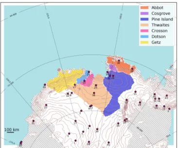
Figure 1. Simulation domain. The drainage basins (Rignot et al., 2019) under consideration in this paper are shaded in color and Au-tomatic Weather Stations (AWSs) are indicated with red points. The hatched area represents ice shelves and contour lines the surface el-evation (every 200 m). Station names from 1 to 41: (1) Brianna, (2) Byrd, (3) Cape Adams, (4) Doug, (5) Elizabeth, (6) Evans Knoll, (7) Harry, (8) Janet , (9) Kominko-Slade, (10) Martha II, (11) Martha I, (12) Mount McKibben, (13) Noel, (14) Patriot Hills, (15) Siple Dome, (16) Ski Hi, (17) Swithinbank, (18) Theresa, (19) Backer Is-land, (20) Bean Peaks, (21) Bear Peninsula, (22) Clarke Mountains, (23) Gomez Nunatak, (24) Haag Nunatak, (25) Howard Nunatak, (26) Inman Nunatak, (27) Kohler Glacier, (28) Lepley Nunatak, (29) Lower Thwaites Glacier, (30) Lyon Nunatak, (31) Mount Pater-son, (32) Mount Sidley, (33) Mount Suggs, (34) Patriot Hills, (35) Steward Hills, (36) Thurston Island, (37) Toney Mountain, (38) Up Thwaites Glacier, (39) Whitmore Mountains, (40) Wilson Nunatak, (41) Russkaya. The relaxation zone is shown in white (∼ 50 km).
(90th percentile) and a mean bias varying from −1.97 to 1.31◦C for the whole year (see Supplement for more details). The model tends to overestimate the lowest observed wind and underestimate the highest observed wind speeds (regres-sions in Fig. 2b). The model agreement with observations is nonetheless good on average, with a mean underestimation of 0.42 m s−1. The statistics per station show a RMSE vary-ing from 1.73 to 3.69 m s−1 and a mean bias varying from −3.08 to 0.85 m s−1for the whole year. The variance of the wind speed simulated by MAR is lower than observed. Less satisfactory results are generally found for the stations lo-cated on an island. This can be explained by the resolution of 10 km, which is still too coarse to resolve small topographic features. For both near-surface temperature and wind speed, the statistics for the summer period (DJF) are very similar to the statistics for the whole year. Our results show very sim-ilar model skills compared to other simulations in the same region (Deb et al., 2018; Lenaerts et al., 2017) or at coarser resolution over the whole ice sheet (Agosta et al., 2019).
Table 1. Correlation between climate indices (−SOI, SAM, ASL longitudinal position, ASL relative central pressure, ASL actual central pressure) in austral summer (DJF). Values in brackets represent the percentage of significance.
ASL relative ASL actual Statistical ASL longitudinal central central correlation (R) −SOI SAM position (◦east) pressure (hPa) pressure (hPa) −SOI −0.45 (99 %) −0.22 (82 %) 0.00 (1 %) 0.40 (99 %)
SAM 0.18 (73 %) −0.25 (88 %) −0.88 (99 %)
ASL longitudinal −0.23 (84 %) −0.15 (63 %) position (◦east)
Figure 2. Scatter plots of observed vs. simulated daily near-surface temperature (a) and daily near-surface wind speed (b) for the selected AWSs (see corresponding locations and names in Fig. 1). The statistics, including RMSE, correlation (R), bias, and standard deviations (σ ), are calculated for individual stations and provided as multi-station mean over the whole year and over the summer months (DJF). The range of RMSE and biases across individual stations is also indicated with the 10th percentile and the 90th percentile of all RMSE values. The lines represent least-mean-square linear fit between simulated data and observations. The complete statistical analyses for individual AWSs are provided in the Supplement (Tables S1–S2).
Figure 3. Annual mean (1979–2017) simulated SMB (blue–green scale) and relative error of the simulated SMB compared to the airborne-radar data from Medley et al. (2013, 2014) (blue–red color bar). Grey contours indicate the surface height (every 1000 m). The drainage basins under consideration are the same as in Fig. 1 (large grey contours here).
We now assess the simulated SMB compared to the SMB from Medley et al. (2013, 2014) derived from airborne radar over the period 1980–2011. The simulated SMB is well ctured by MAR with a mean relative overestimation of ap-proximately 10 % over the Thwaites basin and local errors smaller than 20 % at all locations (Fig. 3). The interannual variability is also well simulated by MAR with a correlation of 0.90 (Fig. 4). In order to have a broad overview of the SMB evaluation, we also compared the simulated SMB with the GLACIOCLIM-SAMBA dataset (Favier et al., 2013) over the Ross and Siple Coast sector (See Fig. S1 in the Sup-plement). The bias of simulated SMB compared to obser-vation SMB is less than 10 mm w.e. a−1 and local bias can
reach 30 mm w.e. a−1. However, the relative bias between the GLACIOCLIM-SAMBA dataset and simulated SMB is more pronounced with only 44 % of GLACIOCLIM-SAMBA sites showing a relative error with simulated SMB lower than 20 %. All SMB components are shown in Table 2.
The areas of highest surface melt (> 100 mm w.e. a−1)are located near the coast and particularly over Abbot,
Cos-Figure 4. Time series of the annual mean (January to Decem-ber) simulated and radar-derived SMB from 1980 to 2011 over the Thwaites basins.
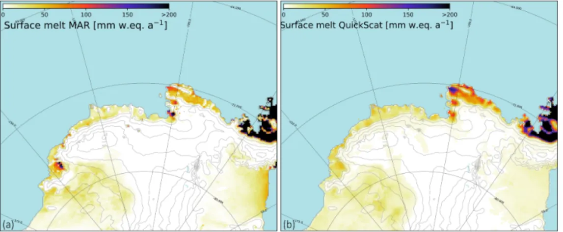
grove and the eastern part of Pine Island ice shelf, while more extreme values (> 200 mm w.e. a−1)are found near the peninsula in both simulated and observed datasets (Fig. 5). Even if the simulated and observed patterns are similar, the simulated surface melt is a factor of 2 lower than observa-tions locally (e.g. over Abbot ice shelf and the peninsula). While the interannual melt rate variability is well reproduced with a correlation of 0.80, the surface melt rate simulated by MAR is underestimated by 18 % on average compared to QuickSCAT estimates (Fig. 6a). Surface melt rate over Pine Island basins is well simulated by MAR (Fig. 6b) with R equal to 0.80 compared to drainage basins with low sur-face melt (i.e. Crosson, Dotson) where R is equal to 0.14 and 0.24, respectively. This melt underestimation, particu-larly pronounced over drainage basins with low surface melt rate, could be explained by the slight overestimation of the snowfall accumulation (10 %–20 %), as the presence of a fresh snow layer of high albedo overlying snow or ice lay-ers of lower albedo likely reduces melt. MAR surface melt presents a slight overestimation over Getz ice shelf (Fig. 5) possibly explained by wind advection, foehn effect or even snow metamorphism simulated by MAR. Further work is needed to understand such local biases. MAR is fully driven by low-resolution ERA-Interim sea ice cover and tempera-ture; therefore possible underestimation of the presence of polynyas can also play a role in the melt biases.
We also compare the number of melt days to the satellite products from Nicolas et al. (2017) and Picard et al. (2007). To avoid no-melt-day areas in the time series computation, we use the area where the annual number of melt days for each dataset is more than 3 melt days per year, which cor-responds approximately to the ice shelf zone. As with the amount of surface melt, the number of melt days over the domain is underestimated by MAR (Fig. 7). The amplitude of the underestimation is not very sensitive to the melt rate threshold used to define a melt day in MAR. A threshold of
1 mm w.e. d−1(as in Datta et al., 2019) gives a mean under-estimation of 4.8 d per year compared to observation from Nicolas et al. (2017), while a threshold of 3 mm w.e. d−1(as in Deb et al., 2018; Lenaerts et al., 2017) gives a mean un-derestimation of 4.9 d per year. This unun-derestimation is less pronounced (0.8 to 0.9 d per year depending on the thresh-old) when using Picard et al. (2007) as a reference. The inter-annual variability in the number of melt days is reproduced with correlations of 0.69 and 0.43 to the two satellite prod-ucts (Fig. 7). Previous study on the Antarctic peninsula also found that MAR melt occurrence is comparable to satellite products, but slightly underestimated over the western coast of the Peninsula (Datta et al., 2019).
Overall, MAR simulates the interannual variability of the Amundsen sector well, and we are now going to use these simulations to investigate the drivers of interannual variabil-ity of SMB and surface melting.
3.2 Drivers of summer interannual variability
In this subsection, we first investigate the large-scale con-ditions leading to interannual anomalies in summer SMB or surface melting. For sake of clarity, we only consider the Pine Island and Thwaites basins (together) as a first approach. To identify large-scale conditions leading to high (low) SMB, we calculate composites defined as the average of summers presenting a SMB greater than the 85th (lower than the 15th) interannual percentile, and we proceed similarly for surface melt composites. We choose the 85th and 15th percentiles to optimize the signal-to-noise ratio.
Sea surface pressure composites show that distinct mecha-nisms affect the interannual variability of summer SMB and surface melting (Fig. 8). Summers with high SMB are on av-erage characterized by a far westward (by ∼ 30◦) and south-ward (by 3–4◦) migration of the ASL center, while the re-verse migration is found for summers with low SMB, al-though with a smaller displacement (∼ 15◦ eastward). In contrast, years with high surface melt rates are character-ized by a much smaller ASL migration, and no migration is found for years with low surface melt rates, but the pres-sure gradients differ between the high and low composites. Therefore, we hereafter consider the variability of SMB and surface melting separately.
To further characterize the tropospheric circulation associ-ated with years of low or high summer SMB, we plot com-posites of both the 500 hPa geopotential height (Fig. 9a, b) and the 500 hPa geopotential height divided by the domain-averaged value for each season (Fig. 9c, d). The latter has the advantage of highlighting changes in regional gradi-ents (related to the regional circulation) rather than larger-scale changes in geopotential height. Both provide simi-lar composites, but the statistical significance is higher in Fig. 9c, d. On average, low-SMB summers are characterized by a northward and eastward ASL migration (shown through a dipole in the 500 hPa normalized geopotential composite
Figure 5. Annual surface melt rate (a) simulated by MAR over 1999–2009 and (b) derived from QuickSCAT satellite data over the same period (Trusel et al., 2013) and interpolated over the MAR grid.
Figure 6. (a) Time series of surface melt rates in mean over the model domain derived from satellite data and simulated by MAR; years labeled on the X axis refer to the second year of a given austral summer (e.g., summer 1999–2000 is labeled 2000). (b) Surface melt modeled versus surface melt interpolated from satellite data (QuickSCAT) over drainage basins (only where surface melt > 0 mm w.e. a−1)and over the period 1999–2009.
in Fig. 9a, c), which is associated with an offshore surface wind anomaly over the glaciers of the Amundsen Sea sector (Fig. 9e). Conversely, high-SMB summers are characterized by a southward and westward ASL migration (Fig. 9b, d), which is associated with an onshore surface wind anomaly over the glaciers of the Amundsen sector (Fig. 9f). The cir-culation anomalies typical of high-SMB summers favor the southward transport of precipitable water as indicated by the composites of integrated vapor transport (Fig. 10a, b). In-creased moisture transport towards the Amundsen Sea Em-bayment leads to denser cloud cover (Fig. 10c, d) and in-creased SMB.
On average, high-melt summers are also associated with increased moisture transport towards the Amundsen Sea Em-bayment and conversely for low-melt summers (Fig. 11a, b), but the mechanism is somewhat different from the case of SMB. The ASL migration during high-melt summers is much smaller than for the high-SMB summers (Fig. 8b). As
previously done for SMB, we plot composites of both the 500 hPa geopotential height (Fig. 12a, b) and the 500 hPa geopotential height divided by the domain-averaged value for each season (Fig. 12c, d), the latter better highlighting regional circulation changes (geopotential gradients). Sum-mers with high surface melt rates show a significant in-crease in the 500 hPa geopotential height over the Belling-shausen Sea (Fig. 12b), i.e. an anticyclonic anomaly, and small westward ASL migration as shown in the 500 hPa nor-malized geopotential composite (Fig. 12d). This anomaly is against the ASL mean circulation and creates a northerly flow anomaly over the ice sheet in the Amundsen sector (Fig. 12e, f). This anticyclonic anomaly was described by Scott et al. (2019) in terms of enhanced blocking activity. As in Scott et al. (2019), we find that high-melt summers are as-sociated with denser cloud cover (Fig. 11c, d) and increased downward longwave radiation (Fig. 11e, f), and therefore surface air warming, while the opposite occurs for low-melt
Figure 7. Time series of the number of melt days per summer (DJF) averaged over the part of the domain with more than 3 melt days per year on average (which approximately corresponds to the ice shelf zone), derived from two satellite products and simulated by MAR (defined using a melt rate threshold of either 1 or 3 mm w.e. d−1).
summers. Composites of sensible heat flux indicate that heat is lost by the snow surface to the atmosphere for high-melt summers, i.e. high melt summers are not caused by foehn events on average (Fig. S2).
Now that we have described the mechanisms in play for summers with high and low SMB or surface melt rates, we investigate the connections between the leading modes of cli-mate variability (ENSO, SAM and ASL variability) and sum-mer SMB and surface melting over the individual Amundsen drainage basins (shown in Fig. 1).
In line with the previous composite analysis for high-and low-SMB composites, the SMB in all the drainage basins is anticorrelated to the ASL longitudinal position (Ta-ble 3, fourth column). This anticorrelation has little statisti-cal significance for Abbot and Cosgrove, but for Dotson and Thwaites the ASL longitudinal position explains nearly 40 % of the SMB interannual variance (explained variance given by square correlations). The ENSO–SMB relationship has moderate levels of statistical significance, with positive SMB correlations to −SOI for all basins but a part of SMB vari-ance explained by ENSO that remains below 16 % (Table 3, second column). −SOI and the ASL longitudinal location are not significantly connected together (Table 1); therefore their connection to SMB can be considered independent from each other. Finally, the SMB is significantly correlated to neither the ASL relative central pressure (Table 3, fifth row) nor the SAM index (Table 3, third column) for all the basins. To bet-ter describe inbet-terplays, we also calculate a multi-linear re-gression of SMB on the four indices (last column of Table 3). Accounting for several indices increases the explained SMB variance compared to a single index, indicating an interplay of the ASL and ENSO. Overall, 16 % to 49 % of the summer
SMB variance (increasing westward) can be explained by a linear combination of the climate indices.
We now investigate similar relationships, but with surface melt rates instead of SMB. By contrast to SMB, the sur-face melt connection to the ASL relative central pressure is stronger than its connection to the ASL longitudinal posi-tion (Table 4, fourth and fifth columns), which again high-lights the two distinct mechanisms explaining high or low melt rates vs. high or low SMB. The part of the melt rate variance explained by the ASL relative central pressure in-creases westward, from 12 % for Abbot to 21 % for Getz. Even though the effect of the ASL central pressure domi-nates, there is still a moderate anticorrelation between melt rates and the ASL longitudinal position, suggesting that the mechanism explaining high and low SMB can explain a small part of the melt rate variance (less than 10 %). In a way similar to SMB, SOI explains less than 9 % of the melt rate’s variance, with moderate statistical significance (Table 4, sec-ond column), and as for summer SMB there is no significant relationship to the SAM. We have repeated the calculations considering the number of melt days, and we find very sim-ilar results in terms of correlations (Table 4, second line in each row). Relatively similar conclusions can be drawn from observational estimates of the number of melt days (values in italic in Table 4), except that satellite estimates indicate a stronger correlation to −SOI, even exceeding the correla-tion to the ASL central pressure in the case for most drainage basins (the variance explained by −SOI reaching 25 %). As the SAM index is significantly anticorrelated to ENSO (Ta-ble 1), the stronger melt–SOI correlation in the observational products goes together with a stronger melt–SAM anticorre-lation than in our simuanticorre-lations. To better describe interplays, we also calculate a multi-linear regression of melt rates on the four indices (last column of Table 4). Accounting for sev-eral indices increases the explained melt rate variance com-pared to a single index, which indicates an interplay of the fours modes of variability. Overall, 21 % to 30 % of the sum-mer melt rate variance can be explained by a linear combina-tion of the climate indices.
The part of explained variance never exceeds 50 % of the summer melt and SMB variance. Possible reasons for this are as follows. (i) The modes of variability do not explain all the variance locally; for example, the leading EOF of sea sur-face temperature (SST) in the equatorial Pacific (representing ENSO) only accounts for 50 % to 70 % of the SST variance (e.g. Roundy, 2014), meaning that the tropical convection thought to influence Antarctica is not completely described by SOI or NINO3.4. (ii) Assuming that a large part of the tropospheric circulation variability is explained by ENSO, SAM and ASL indices, there are reasons why the connection may be weaker for SMB and surface melting because of their nonlinear dependence on sea ice and evaporation in coastal regions, the evolution of snow properties, etc. (iii) Strong modulation of the southeast Pacific extratropical circulation by Rossby wave trains is not only due to the existence of El
Figure 8. Summer sea surface pressure composites for high–low SMB (a) and high–low surface melt (b). The ice sheet height is indicated by thin grey contours (every 500 m).
Table 2. Annual SMB decomposition for all drainage basins over 1979–2017 with SMB = snowfall + rainfall − sublimation − runoff. The middle rows indicate other terms that are not directly part of the SMB. The last two rows give snowfall and melt rates averaged over the ice shelves.
(mm w.e. yr−1) Abbot Cosgrove Pine Island Thwaites Crosson Dotson Getz
SMB 959.5 660.5 429.1 504.5 867.7 895.0 843.0 Sublimation 26.5 30.3 12.7 0.6 22.6 25.6 22.8 Snowfall 981.9 688.5 441.3 505.0 887.6 919.5 864.9 Rainfall 4.0 2.3 0.4 0.1 2.8 1.1 0.8 Runoff 0.0 0.0 0.0 0.0 0.0 0.0 0.0 Refreezing 36.4 27.0 4.3 1.0 6.2 7.2 9.6 Surface melt 32.5 24.8 3.9 0.9 3.4 6.1 8.8
Snowfall (only over ice shelf) 795.4 296.9 422.7 811.5 1051.5 672.0 789.9 Surface melt (only over ice shelf) 57.9 83.2 82.0 26.5 18.5 23.7 26.7
Niño events but also depends on the exact spatial distribu-tion of deep convecdistribu-tion in the tropical central Pacific and the strength of the polar jet (Harangozo, 2004). (iv) A part of the variability of SMB and melting may be stochastic, i.e. not necessarily driven by variability with spatiotemporal coher-ence at large scales.
4 Discussion
The composite analysis and the correlation of SMB and melt rates to the ASL indices give a consistent picture. Summers tend to be associated with high SMB when the ASL migrates westward and southward because this places the northerly flow (ASL eastern flank) over the Amundsen Sea, thereby increasing the southward humidity transport and snowfall. This corresponds to the large-scale features described by Hosking et al. (2013) but is here described for the SMB of individual drainage basins. By contrast, longitudinal migra-tions of the ASL are not the main driver of surface melting variability, as previously noted by Deb et al. (2018). Sum-mers tend to be associated with high surface melt rates when
the Amundsen–Bellingshausen region experiences blocking, i.e. anticyclonic conditions, which tends to decrease the cli-matological southerly flow (western flank of the ASL) and to favor marine air intrusions that make cloud cover denser with increasing downward longwave radiation, as described by Scott et al. (2019).
While the role of the ASL now appears to be quite clear, the exact impact of ENSO on SMB and surface melt rates re-mains elusive. Earlier studies analyzing the impact of ENSO on precipitation in West Antarctica had difficulties under-standing the mechanisms and the robustness of the signal, because they had to rely on relatively short observation and reanalysis periods (Bromwich et al., 2000; Cullather et al., 1996; Genthon and Cosme, 2003). Using a dedicated SMB model over a longer time period, we have shown here that the ENSO–SMB relationship in austral summer exists, but it is relatively weak as SOI alone cannot explain more than 16 % of the interannual variance in summer SMB. The re-lationship between ENSO and the number of melt days was identified by Deb et al. (2018) using both regional simula-tions and a satellite product. It was then thoroughly described
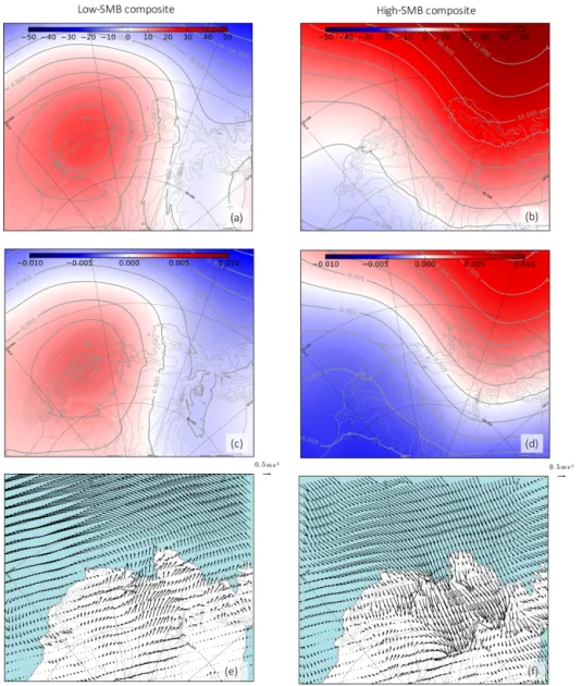
Figure 9. (a, b) The 500 hPa geopotential height (m), (c, d) 500 hPa geopotential height divided by the domain-averaged value for each season and (e, f) 10 m wind (m s−1)anomalies during low-SMB summers (left) and high-SMB summers (right); scales of arrow lengths are shown near the upper right corner of panels (e) and (f). Anomalies are calculated as high or low composites minus the climatology over 1979–2017. The hatched area (a–d) represents significance > 90 % calculated with Welch’s t test.
Table 3. Correlation R between ENSO, SAM, and ASL indices and the SMB over individual drainage basins in austral summer. The statistical significance (Welch’s t test) is written within brackets. The last column shows the correlation of a multi-linear regression to the four indices using a least absolute shrinkage and selection operator (LASSO; Tibshirani, 1996).
ASL relative
Drainage −SOI vs. SAM index ASL longitudinal central pressure Multi-linear basins SMB vs. SMB location vs. SMB vs. SMB regression Abbot 0.25 (87 %) 0.14 (59 %) −0.15 (65 %) −0.01 (3 %) 0.40 Cosgrove 0.26 (88 %) 0.16 (65 %) −0.21 (80 %) 0.08 (36 %) 0.46 Pine Island 0.32 (95 %) 0.03 (17 %) −0.25 (87 %) −0.17 (69 %) 0.47 Thwaites 0.33 (96 %) 0.02 (8 %) −0.45 (99 %) −0.10 (47 %) 0.57 Crosson 0.40 (99 %) −0.00 (2 %) −0.53 (99 %) −0.14 (60 %) 0.66 Dotson 0.36 (97 %) 0.00 (2 %) −0.61 (99 %) 0.15 (65 %) 0.70 Getz 0.30 (93 %) −0.15 (62 %) −0.64 (99 %) 0.27 (90 %) 0.68
Table 4. Correlation R between −SOI, SAM, and ASL indices and MAR surface melt rates (bold), MAR number of melt days (regular), number of melt days from satellite products (italic, first value for Nicolas et al. (2017) and second for Picard et al. (2007)), over individual ice shelves in summer. The statistical significance (Welch’s t test) is written within brackets. The last column shows the correlation of a multi-linear regression to the four indices using a least absolute shrinkage and selection operator (LASSO, Tibshirani 1996).
Drainage SAM ASL longitudinal ASL relative Multi-linear basins −SOI index location central pressure regression Abbot 0.23 (84 %) −0.05(24 %) −0.25(86 %) 0.35 (97 %) 0.46 0.25 (86 %) −0.04 (19 %) −0.23 (84 %) 0.30 (93 %) 0.44 0.37 (97 %) −0.22(79%) −0.29(91%) 0.32 (94 %) 0.49 0.37 (98 %) −0.18(71%) −0.18(72%) −0.24(92%) 0.47 Cosgrove 0.24 (86 %) −0.08(36 %) −0.30(93 %) 0.37 (98 %) 0.50 0.25 (87 %) −0.06 (29 %) −0.29 (92 %) 0.32 (95 %) 0.47 0.37 (97 %) −0.20(76%) −0.37(97%) 0.32 (94 %) 0.52 0.38 (98 %) −0.25(87%) −0.16(65%) 0.27 (90 %) 0.46 Pine Island 0.30 (86 %) −0.07(33 %) −0.31(94 %) 0.38 (98 %) 0.54 0.29 (92 %) −0.03 (13 %) −0.34 (96 %) 0.35 (97 %) 0.55 0.48 (99 %) −0.29(91%) −0.21(78%) 0.42 (99 %) 0.62 0.44 (99 %) −0.19(75%) −0.13(56%) 0.37 (98 %) 0.59 Thwaites 0.29 (92 %) −0.13(56 %) −0.25(87 %) 0.39 (98 %) 0.51 0.35 (95 %) −0.11 (43 %) −0.19 (69 %) 0.51 (99 %) 0.67 0.48 (99 %) −0.23(81%) −0.11(45%) 0.29 (91 %) 0.55 0.44 (99 %) −0.28(89%) −0.06(26%) 0.26 (87 %) 0.52 Crosson 0.28 (91 %) −0.14(60 %) −0.23(84 %) 0.41 (99 %) 0.51 0.29 (86 %) −0.08 (30 %) −0.11 (42 %) 0.40 (97 %) 0.52 0.48 (99 %) −0.35(95%) −0.20(76%) 0.39(98 %) 0.61 0.35 (96 %) −0.35(96%) −0.10(45%) 0.41 (98 %) 0.52 Dotson 0.27 (90 %) −0.14(60 %) −0.24(86 %) 0.42 (99 %) 0.52 0.26 (86 %) −0.13 (54 %) −0.25 (86 %) 0.44 (99 %) 0.53 0.36 (95 %) −0.27(84%) −0.03(11%) 0.36 (94 %) 0.52 0.33 (93 %) −0.28(86%) 0.13 (51 %) 0.32 (91 %) 0.50 Getz 0.22 (82 %) −0.16(65 %) −0.26(88 %) 0.46 (99 %) 0.53 0.22 (82 %) −0.16 (67 %) −0.29 (92 %) 0.46 (99 %) 0.54 0.50 (99 %) −0.42(99%) −0.24(84%) 0.41 (99 %) 0.64 0.34 (96 %) −0.41(98%) −0.15(63%) 0.34 (96 %) 0.46
by Scott et al. (2019), who found that SOI could explain 20 % of the melt variance when considering all the Amundsen ice shelves together and using satellite products (correlation of 0.45 in their Table 3). While we obtain results similar to those of Scott et al. (2019) when using the number of melt days derived from satellite products, both the number of melt days and the melt rates simulated by MAR indicate less vari-ance explained by SOI, that is, between 5 % and 9 % for the individual drainage basins. Our MAR simulations certainly contain biases in the representation of the melting process and the way it affects surface properties such as albedo and roughness, but it is also possible that the number of melt days derived from microwave satellite data is biased due to vari-ability in surface conditions, percolation within fresh snow, meltwater ponding (observed on Pine Island; Kingslake et al., 2017) and satellite overpass time (Tedesco, 2009; Scott
et al., 2019). More work will be needed to understand these differences.
Numerous publications have explained the remote effects of ENSO on the West Antarctic climate through Rossby wave trains that connect the convective anomalies associated with ENSO in the equatorial Pacific to Antarctica (e.g., Yuan and Martinson, 2001). However, austral winter and spring con-ditions are more favorable for Rossby wave trains to be formed and to propagate to high southern latitudes than sum-mer conditions (Harangozo, 2004; Lachlan-Cope and Con-nolley, 2006; Ding et al., 2011, and references therein). The poleward propagation of tropically sourced Rossby waves in summer is indeed inhibited by the strong polar front jet in the South Pacific sector at that time of the year, which leads to Rossby wave reflection away from the Amundsen Sea region (Scott Yiu and Maycock, 2019). This lack of direct
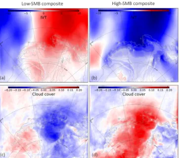
Figure 10. (a, b) Vertical integrated vapor transport (IVT) along the y axis (negative toward the continent) calculated as IVT [kg m−2] =R700
925 q · vdPg , with q the specific humidity (g kg−1),
vthe wind speed (m s−1), P the pressure (Pa), and g the gravity (9.81 m s−2)and (c, d) cloud cover (no units, from 0 to 1) anomalies during low-SMB summers (left) and high-SMB summers (right). Anomalies are calculated as high or low composites minus the cli-matology over 1979–2017. The hatched area represents significance >90 % calculated with Welch’s t test.
connection in summer was supported by Steig et al. (2012), who found the weakest correlations between NINO3.4 and wind stress anomalies in the Amundsen Sea in DJF com-pared to other seasons. Therefore, we investigated possible lags in the relationships to ENSO. While ENSO peaks in DJF, it starts to develop in MAM (March–April–May), as indicated by the growing SOI autocorrelation from a 9- to 6-month lag (Fig. 13a). The first implication of this is that any signal correlated to SOI in DJF will be correlated to SOI in the previous JJA without the need for a lagged physical mechanism. Nevertheless, the correlation between SMB or melt rates in DJF and SOI in the preceding JJA is higher than the synchronous correlation for all the drainage basins (solid curves in Fig. 13b–h), which suggests that the lagged relationship is not only a simple statistical artifact. The re-sults of Ding et al. (2011) and Steig et al. (2012) suggest that there could be a lagged mechanism whereby ENSO would influence West Antarctica in austral spring or winter, with a delayed response of SMB and melting in the following aus-tral summer. The number of melt days derived from satellite data also gives 6-month-lagged correlations to SOI that are as high or higher than synchronous correlations for most ice shelves (dashed curves in Fig. 13b–h).
We now discuss possible explanations for this lag. As mentioned previously, the Rossby wave trains connecting the equatorial Pacific to Antarctica are expected to develop
Figure 11. (a, b) Vertical integrated vapor transport (IVT) along the y axis (negative toward the continent (kg m−2, same formula as for Fig. 10), (c, d) cloud cover (no units, from 0 to 1) and (e, f) downward longwave radiation (W m−2)anomalies during low-melt summers (left) and high-low-melt summers (right). Anomalies are calculated as high or low composites minus the climatology over 1979–2017. The hatched area represents significance > 90 % cal-culated with Welch’s t test.
within a few weeks in response to ENSO convective anoma-lies (e.g. Hoskins and Karoly, 1981; Mo and Higgins, 1998; Peters and Vargin, 2015). Therefore, the lag has to come from anomalies stored in a slower medium, such as snow-pack, ocean or sea ice. Snow surface melting in DJF is cor-related neither to the temperature of snow layers within the first 2 m in the previous months (not shown) nor to the snow accumulated over the previous months (not shown). This in-dicates that heat diffusion in snow or preconditioned poros-ity or albedo of snow is not responsible for the 6-month lag. By contrast, we find that El Niño events in JJA sig-nificantly reduce the sea ice cover in the following DJF (Fig. 14). This is reminiscent of Clem et al. (2017), who found stronger lagged correlation between SON ENSO and DJF sea ice cover than synchronous correlation in DJF, with consequences on summer air temperatures. We suggest two possible explanations for this lagged ENSO–sea ice relation-ship. First, it could be slowly advected from the Ross Sea. Pope et al. (2017) indeed found that El Niño events
develop-Figure 12. (a, b) The 500 hPa geopotential height (m) and (c, d) 500 hPa geopotential height divided by the domain-averaged value for each season and (e, f) 10 m wind (m s−1)anomalies dur-ing low-melt summers (left) and high-melt summers (right); scales of arrow lengths are shown near the upper right corner of panels (e) and (f). Anomalies are calculated as high or low composites mi-nus the climatology over 1979–2017. The hatched area represents significance > 90 % calculated with Welch’s t test.
ing in MAM created a dipole of sea ice anomalies, with de-creased (inde-creased) concentration in the Ross Sea (Amund-sen and Bellingshau(Amund-sen seas). Using a novel sea ice budget analysis, they showed that the decreased concentration in the Ross Sea was then advected eastward, reaching the Amund-sen Sea in SON and DJF.
There is also another possible pathway for a lagged ENSO–sea ice relationship. The zonal wind stress over the Amundsen Sea continental shelf break is a good proxy for the transport of Circumpolar Deep Water (CDW) onto the continental shelf (Thoma et al., 2008; Holland et al., 2019). Steig et al. (2012) noted significant correlations between wind stress and ENSO in JJA and SON but not in DJF. All these studies as well as Paolo et al. (2018) pointed out scales of a few months for the buildup and advection of CDW on the continental shelf and then into the ice shelf cavities where they produce basal melting, and Paolo et al. (2018) reported correlations between ENSO and ice shelf thinning 6 months later. As stronger ice shelf melt rates tend to decrease sea ice in this region due to the entrainment of warm CDW towards
the surface (Jourdain et al., 2017; Merino et al., 2018), the connection through CDW intrusions may also explain a part of the lag between ENSO and DJF sea ice in the Amundsen Sea. We suggest that both mechanisms (eastward advection of sea ice anomalies and anomalous intrusions of CDW) may explain the 6-month lag between DJF SMB or melting and ENSO, and we leave the details of the ocean–sea ice pro-cesses for future research.
Beyond the ASL and ENSO, we also find that the SAM is not significantly related to summer SMB and sur-face melt over individual drainage basins at interannual timescales, which agrees with Deb et al. (2018). This may appear contradictory to the results obtained by Medley and Thomas (2019), showing that the positive SAM trend from 1957 to 2000 largely explains the pattern of annual SMB trends over the Antarctic ice sheet. First of all, their resid-ual SMB trend (i.e. not related to SAM) is particularly strong in the Amundsen Sea Embayment (their Fig. 1e), highlight-ing that only a part of the SMB trend in that region may be related to the SAM trend. The multi-decadal SAM trend is also related to ozone depletion and emissions of greenhouse gases, and the interannual SAM variability may have differ-ent characteristics and impacts on SMB. Furthermore, the ab-sence of a SMB–SAM relationship in our MAR simulations is specific to the austral summer, which represents 15 % of the annual SMB, and correlations are more significant for the other seasons (Table S3). Therefore, the significant SAM– SMB relationship suggested by Medley and Thomas (2019) for annual SMB is not necessarily contradictory to our re-sults. Lastly, previous studies have suggested that the SAM– ENSO anticorrelation may diminish the impact of ENSO on surface melting and SMB. Partial correlations used to disen-tangle the SAM and ENSO influences on SMB do indicate a slightly stronger SMB–ENSO correlation when the effect of SAM is removed (in particular for Abbot and Cosgrove; see second and third columns of Table 5), but the effect is relatively small. For melt rates, the SAM modulation is very weak for all the basins (Table 5, fourth and fifth columns).
Lastly, we discuss the relationship between surface melt and snowfall over the ice shelves of the Amundsen sector (last rows of Table 2). According to Table 2, runoff is null over all the ice shelves, which means that the firn is never saturated. In other words, all surface meltwater and rainfall refreeze within the firn. This is consistent with Pfeffer et al. (1991), who estimated that the melt rate needed to sat-urate the firn with water and lead to hydrofracturing can be estimated as 0.7 times the snowfall rate (both melt and snow-fall rates expressed in kilograms per square meter per second or millimeter water equivalent). This indicates that meltwa-ter ponding and complex surface hydrological flows are un-likely to develop over West Antarctic ice shelves under the current climate. To reach saturation at the scale of the entire ice shelf in the future (and therefore to initiate hydrofractur-ing), the 0.7 ratio of Pfeffer et al. (1991) suggests that melt
Table 5. Partial correlation of −SOI vs. SMB or melt rates, removing the influence of SAM (columns 2 and 4). Corresponding full correlations are indicated in columns 3 and 5 (same as Tables 3 and 4).
Partial correlation Partial correlation
Drainage −SOI vs. SMB −SOI vs. surface melt Correlation −SOI basins (without SAM) −SOI vs. SMB −SOI vs. SMB (without SAM) vs. surface melt
Abbot 0.36 0.25 0.21 0.23 0.23 Cosgrove 0.37 0.26 0.21 0.23 0.24 Pine Island 0.38 0.32 0.26 0.30 0.30 Thwaites 0.38 0.33 0.23 0.25 0.29 Crosson 0.45 0.40 0.29 0.24 0.28 Dotson 0.40 0.36 0.25 0.23 0.27 Getz 0.26 0.30 0.18 0.17 0.22
Figure 13. Correlation between lagged 3-month averaged −SOI (i.e. DJF at zero lag, previous JJA at −6 lag) and (a) DJF SOI. (b–h) Simulated SMB and melt rates in individual drainage basins. The dashed curves correspond to the number of melt days derived from satellite data by Picard et al. (2007).
rates would need to be multiplied by 2.5 (Cosgrove) to 40 (Crosson) compared to present conditions.
5 Conclusions
In this paper we have analyzed possible drivers for summer surface melt and SMB interannual variability over the last decades in the Amundsen sector, West Antarctica. For this, we have simulated the 1979 to 2017 period with the
Re-Figure 14. Summer sea ice cover (%) anomaly (composites minus the climatology over 1979–2017) during El Niño events in JJA (6 months before). Contours represent significance with Welch’s t test.
gional Atmosphere Model, MAR. We have first evaluated our model configuration in comparison to observational products (i.e. AWS, airborne-radar and firn-core SMB, melt days from satellite microwave, and melt rates from satellite scatterom-eter). MAR gives good results for near-surface temperatures (mean overestimation of 0.10◦C), near-surface wind speeds (mean underestimation of 0.42 m s−1)and SMB (local rela-tive bias < 20 % over the Thwaites basin). The mean surface melt rate over the Amundsen Sea region is underestimated by 18 % compared to the estimates derived from QuickSCAT (Trusel et al., 2013), and the interannual variability of sur-face melting is relatively well reproduced in terms of melt rate (R = 0.80) or number of melt days (R = 0.43 to 0.69 depending on the satellite product) as also found by previous studies using the same MAR version (i.e. Datta et al., 2019). Similar underestimation was also found in another regional atmospheric model of the Amundsen region (underestima-tion of 30 %–50 % found by Lenaerts et al., 2017). Overall,
our results indicate that MAR is a suitable tool to study in-terannual variability in the Amundsen sector.
Then, we have analyzed the interannual variability of sum-mer SMB. The strongest sumsum-mer SMB occurs over Thwaites and Pine Island glaciers when the ASL migrates far westward (by typically 30◦) and southward (by typically 3–4◦). This promotes a southward flow on the eastern flank of the ASL, towards the glaciers, with resulting increased moisture con-vergence, precipitation and therefore SMB. Our study hence provides further support for the connection between Antarc-tic precipitation and the ASL longitudinal position that was previously described by Hosking et al. (2013) based on the ERA-Interim reanalysis. In terms of climate indices, this cor-responds to an anticorrelation between SMB and the ASL longitudinal position. This anticorrelation is found for all the drainage basins of the Amundsen Sea Embayment, and the part of the SMB variance explained by the ASL longitudinal migrations ranges from 2 % to 41 % (increasing westward). A small part of the SMB variance is also related to ENSO, with higher SMB during El Niño events and lower SMB dur-ing La Niña, but less than 8 % of the SMB variance is ex-plained by ENSO variability. This SMB connection to ENSO is independent from its connection with the ASL longitudinal position.
We have also analyzed the interannual variability of sum-mer surface melt rates. The strongest surface melting occurs over Thwaites and Pine Island glaciers when the ASL under-goes an anticyclonic anomaly (likely the signature of block-ing activity), which is visible through anomalies of the ASL relative central pressure. Such an anomaly promotes a south-ward anomaly of near-surface winds and moisture conver-gence over the Amundsen Sea Embayment. As recently de-scribed by Scott et al. (2019), this leads to increased cloud cover and downward longwave radiation, which in turn in-creases surface melting. As for SMB, we do not find that surface melt rate variability in our simulations is strongly connected to ENSO as it does not explain more than 9 % of the total variance in simulated summer surface melt rate (or 12 % of the number of melt days). By contrast and for un-known reasons, the variance in number of melt days derived from satellite products indicates that as much as 25 % of the variance in these products could be explained by −SOI.
We also suggest that at least a part of the ENSO–SMB and ENSO–melt relationships in summer is inherited from the previous austral winter (JJA). Rossby wave trains gener-ated by convective anomalies relgener-ated to developing El Niño events in austral winter significantly affect the Antarctic re-gion, and we suggest that this has some impact on SMB and surface melting in the Amundsen sector 6 months later. Such a delay could be related either to sea ice anomalies gener-ated by ENSO in the Ross Sea in austral winter and taking 6 months to be advected to the Amundsen Sea (Pope et al., 2017) or to marine intrusions of Circumpolar Deep Water that are favored by El Niño events in austral winter (Steig et al., 2012). Circumpolar Deep Water may take 6 months
to reach ice shelf cavities where increased basal melting fa-vors the entrainment of this water towards the ocean surface (Jourdain et al., 2017). It should nonetheless be noted that even accounting for this 6-month lag, the influence of ENSO on summer SMB and melt rates remains weak, not explain-ing more than 15 % variance.
Lastly, we propose that the rate of surface water needed to saturate the firn and lead to hydrofracturing has to increase by a factor of 2.5 to 40 depending on the ice shelf. Such an increase could be reached under strong warming scenarios given the exponential temperature dependence described by Trusel et al. (2015), although snowfall is also expected to in-crease (Krinner et al., 2008; Agosta et al., 2013; Ligtenberg et al., 2013; Lenaerts et al., 2016; Palerme et al., 2017), re-quiring even more meltwater to reach saturation. In their pro-jections, Kuipers Munneke et al. (2014) found that the west-ern part of Abbot as well as Cosgrove could become water-saturated before the end of the twenty-second century, but the other ice shelves of the Amundsen sector remained non-saturated. Further work will be needed to assess the robust-ness of these projections, with other firn models and global projections.
Code and data availability. The MAR code (version 3.9.1) is avail-able on the MAR website (http://mar.cnrs.fr/, last access: 17 Jan-uary 2020); outputs from the Amundsen simulation presented in this study are available on https://doi.org/10.5281/zenodo.2815907.
Supplement. The supplement related to this article is available on-line at: https://doi.org/10.5194/tc-14-229-2020-supplement.
Author contributions. The study was designed by MD-M and NCJ. Setup of the MAR domain configuration was made by MD-M, CA, AD and NCJ. CA, XF, HG, CK and CA developed and tuned the MAR model for Antarctica, and they contributed to improving and interpreting our simulations. CK developed the scripts used to com-pare MAR to AWS data. JDW and VF contributed to the interpreta-tion of our results related to interannual variability. All the authors significantly contributed to this paper.
Competing interests. The authors declare that they have no conflict of interest
Acknowledgements. This work was funded by the French National Research Agency (ANR) through the TROIS-AS (ANR-15-CE01-0005-01) project. The development of MAR was partly funded by Labex OSUG@2020 (ANR10 LABX56) through the “Tout le Monde se MAR” project. All the computations presented in this paper were performed using the GRICAD infrastructure (https:// gricad.univ-grenoble-alpes.fr, last access: 17 January 2020), which is partly supported by the Equip@Meso project (ANR-10-EQPX-29-01) of the program “Investissements d’Avenir” supervised by