Pressure and velocity on an ogee spillway crest operating at high head ratio: experimental measurements and instrumentation

1 INTRODUCTION

Uncontrolled ogee spillways are commonly used as flood release structures on dams. Their shape is de-signed regarding a given upstream head, the design head Hd, so that a zero relative pressure is obtained all along the crest profile (Hager 1987; USBR 1987) when the corresponding design discharge flows over the weir.

In the literature, few studies focused on the flow characteristics over an ogee spillway crest for heads largely greater than the design head. Yet, with the current review of the safety criteria of hydraulic struc-tures due to the availability of longer statistic chronicles, the forecasted increase in frequency and ampli-tude of extreme meteorological events and the evolution of the calculus methods, numerous existing spillways might be considered to face higher heads than the initial design head (Millet et al. 1988; Xlyang and Cederström 2007).

Among the available references, very few studies deal with the flow dynamics and only the upstream head and the pressure along the weir-profile are generally measured. Rouse and Reid (1935) assessed the influence of the crest shape by comparing the discharge coefficients and the pressure distributions of three different ogee spillway profiles with those of a sharp crested weir until a head ratio, H/Hd, equal to three (H = upstream head). Abecasis (1970) and Cassidy (1970) focused their investigations on a proce-dure to control the minimal pressure that occurs on an ogee spillway designed following the recommen-dations of USBR (1948) until a head ratio of three. Vermeyen (1991; 1992) studied, in the frame of a dam project, an ogee-spillway operational until a head ratio of five, but here again no information is available regarding the velocity distribution in the flow. After these previous studies, no more occurrences of

stud-Pressure and velocity on an ogee spillway crest operating at high head

ratio: experimental measurements and validation

Y. Peltier

, B. Dewals

, P. Archambeau

, M. Pirotton

& S. Erpicum

1 _{University of Liege, ArGEnCo Department, Research Group on Hydraulics in Environnmental and Civil}

Engineering (HECE), Liege, Belgium E-mail: S.Erpicum@ulg.ac.be

ABSTRACT: This paper aims at validating pressure and velocity measurements conducted in two physi-cal sphysi-cale models of an ogee spillway crest operating at heads largely greater than the design head. The de-sign head of the second model is 50% smaller than the one of the first model. No piles effect or air en-trance is considered in the study. The velocity field is measured by Large Scale Particle Image Velocimetry. The relative pressure along the spillway crest is measured using pressure sensors. Compari-sons of measured velocities between both spillways indicate low scale effects, the scaled-profiles collaps-ing in most parts of the flow. By contrast, measurements of relative pressure along the spillway crest dif-fer for large heads. A theoretical velocity profile based on potential flow theory and expressed in a curvilinear reference frame is then fitted to the velocity measurements, considered as reference, for ex-trapolating the velocity at the spillway crest. Comparing the extrapolated velocity at the spillway crest and the velocity expressed from the relative pressure finally emphasizes that bottom pressure amplitudes are overestimated for the large spillway, while an averaging effect might operate for the pressure meas-urements on the small spillway.

Keywords: ogee-crested weir, LSPIV, physical modeling, potential flow theory, pressure sensors, scale model.

ies dealing with ogee spillway working at high-head ratio can be found in the literature. The few studies we have found deal with other type of crests, e.g. round crest (Castro-Orgaz, 2008). The knowledge of the velocity field is yet paramount for better understanding the phenomena that drive the flow dynamics in the vicinity of the spillway and to validate the pressure measurements.

Within the framework depicted here-above, the study presented in this paper concerns the validation of velocity and pressure measurements conducted in 2 physical models with different scale factor of an ogee spillway crest operating at head ratios largely greater than one. In this study, no piles effect or air en-trance is considered. The experimental setup, the selected crest profile, the measurement techniques and the theoretical background are presented in section 2. Then, the results are presented in section 3 and compared with theory in section 4 in order to be validated.

2 MATERIAL AND METHOD

2.1 Experimental facility

The main purpose of the project is to reproduce in a controlled environment flows over ogee spillways for heads much higher than the design head. To achieve this, high specific discharges are necessary. Due to the available discharge capacity in the laboratory and to the choice of a model of 20 cm wide in order to minimize wall effects, a maximum design head of 15 cm was possible. Regarding real-life weirs, the di-mensions of the present experiment roughly correspond to one tenth of prototypes.

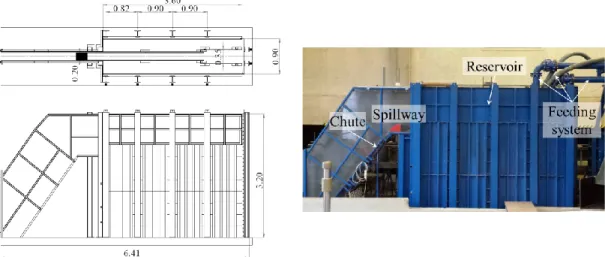
Figure 1. photograph, plan and section views of the experimental facility. Dimensions are in meter.

In the present experiments, the use of a pressure chamber and of another fluid than water was not pos-sible. Therefore, similarities in term of atmospheric pressure and surface tension could not be respected. The experimental facility was made of a large reservoir with an inner width of 0.90 m, a length of 4.00 m and a height of 3.20 m. At the extremity of the reservoir, a removable spillway with a vertical upstream face and a smooth chute was set (Figure 1). The chute was 4.5 m long in order to avoid any backwater ef-fects on the flow in the vicinity of the crest.

The spillway profile being the key-parameter, geometric effects had to be minimized in order to obtain results as general as possible and independent from the scale of the experiment:

• Walls in polyvinyl chloride (PVC) were added in the reservoir for reducing the flow section to the width of the spillway: B = 0.20 m. The flow was thus confined in a 2D-vertical slice passing by the centreline of the spillway and contraction effects affecting the nappe stability were then avoided. The deformation of the new reservoir geometry was minimized by ensuring equality between the hydrostatic pressure distributions on both sides of the walls, through holes at the bottom of the PVC plates.

• Given the maximum design head of 0.15 m and the dimensions of the experimental facility, the ex-pected maximum head over the spillway-crest, Hmax, was found approximately equal to 0.75 m dur-ing the design phase. The independence of the spillway performance from the height of the up-stream face of the spillway, huf, was ensured by setting huf equal to 3Hmax (Melsheimer and Murphy 1970; Reese and Maynord 1987).

The feeding of the reservoir was performed in closed-loop, with one to three regulated pumps bringing the water through one to three pipes depending on the desired discharge. The pipes were terminated by a strainer, which allowed the injection of the water on the whole water column.

2.2 Spillway profiles

Two ogee spillways were constructed for this study. Their geometry follows the standards defined in the book “Hydraulic Design Criteria” (USACE 1987), i.e. the so-called “Waterways Experiment Station (WES) geometry”, as also reported in USBR (1987). Consequently, the upstream quadrant is designed with 3 arcs of circle (see the coordinate in Table 1) and the downstream quadrant follows the power-law equation (1).

1.85 ₂ 0.85

d

x   H z

(1) where in the Cartesian coordinate system, x, y and z are the streamwise, spanwise and vertical directions

respectively; (x, y, z) = (0, 0, 0) at the crest. The z-axis is directed in the upward direction. Table 1. Coordinates for upstream quadrant (USACE 1987).

____________________________________________________________________________________________ x/Hd 0 -0.0500 -0.1000 -0.1500 -0.1750 -0.2000 -0.2200 -0.2400 -0.2600 -0.2760 -0.2780 -0.2800 -0.2818 z/Hd*0 -0.0025 -0.0101 -0.0230 -0.0316 -0.0430 -0.0553 -0.0714 -0.0926 -0.1153 -0.1190 -0.1241 -0.1360 ____________________________________________________________________________________________ * The z-axis is oriented in the upward direction.

The design head of the first spillway, W1, was set to 0.15 m, with a slope for the chute equal to 51°. The geometry of W2 was identical to W1, but a design head of 0.10 m was considered in order to be able to reach higher head ratios for the same discharges. This difference in scale was also used to identify the presence of possible scale-effects.

2.3 Measuring techniques

For each spillway, the flow dynamics was measured and analysed for five head-ratios, H/Hd, ranging from one two five, by step of unity. The upstream head, the pressure along the spillway and the velocity field in the vicinity of the spillway were measured.

2.3.1 Upstream head (water depth and discharge)

The upstream head, H, being the main parameter of the study, the measurement cross-section was chosen with care. It was positioned at a distance from the spillway-crest equal to at least twice the maximal head over the spillway, i.e. xm = 1.5 m. At this distance, the feeding pipes and the spillway have low influences on the velocity profile in the reservoir, which is therefore quasi-uniform on the vertical. Under such flow conditions, the head was easily evaluated by measuring the water depth, h, relative to the crest of the spillway and by adding a term of kinetic energy calculated with the discharge velocity, V, equal to the ra-tio of the discharge, Q, to the area of the measurement cross-secra-tion (see Equara-tion (2)).





each pipe. The uncertainty on the discharge, Q, was equal to 0.7 L.s-1 _{with one pump, to 0.98 L.s}-1 _with

two pumps and to 1.11 L.s-1 with three pumps.

The water depth was measured at x = xm, using an ultrasonic probe (PICO+100). The precision on the measurement, h, was estimated to ±1 mm by calibration tests.

2.3.2 Velocity fields

The velocity fields were obtained by means of Large Scale Particle Image Velocimetry (LSPIV), which is a technique based on the classical PIV techniques and is adapted to be used in large facilities without the use of a laser (Hauet 2009; Hauet et al. 2008b).

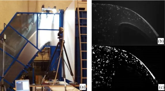
Air-bubbles of approximately 5 mm in diameter were used as seed. Given the velocity in the zone of interest, it was assumed that the bubbles have no relative motions compared to the ambient flow. The bubbles were lighted up using white lights focused above the spillway centreline and a high-speed video camera (Basler A504k) laterally positioned was used to record their displacements (Figure 2a). The expo-sure time of the camera was set to 500 µs with a sampling frequency of 400 Hz and the field of interest was saturated of light. These setting for the camera were chosen to:

• accurately capture air bubbles,

• minimize particle-motions on each frame,

• ensure a reasonable maximum displacement of pixels between two successive frames (max 20 pix-els).

The frames of the resulting video-sequences were then extracted at the same sampling rate and each image was post-processed using ImageMagick (http://www.imagemagick.org), (Figure 2b-c). Each image was orthorectified and georeferenced, resulting in post-processed images in which one pixel was equal to a square of 1 mm side. Finally, using the homemade LSPIV code, the pixel displacements were assessed.

Figure 2. (a) LSPIV set-up. (b) Raw image. (c) Post-processed image.

The mean velocity fields were then obtained from the averaging of 5000 instantaneous velocity fields; with a theoretical uncertainty of at least 6% (Hauet et al. 2008a). Spurious vectors in the mean velocity fields were identified using a median filters (Westerweel and Scarano 2005) and were then simply re-moved.

2.3.3 Pressure

Eighteen relative pressure transducers (KELLER PR23Y) with a measurement range between -5 m to +2 m in relative pressure were distributed along the centreline of the spillway on the weir crest. They gave 1 kHz measurements of the relative pressure through holes of 2 mm diameter. The uncertainty of the pres-sure meapres-surement was found equal to ±20 mm by calibration tests.

2.4 Theoritical profiles of velocity

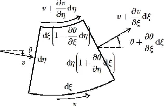
Let us consider an elementary volume of fluid between two streamlines. The streamwise and normal di-rections are denoted by  and  respectively (Figure 3) in a curvilinear reference frame. With v being the norm of the velocity and  indicating the local direction of the flow, the circulation around this element of volume is (Oertel 2010): d d  v +d d   v          (3) (b) (c) (a)

Figure 3. Element of volume between two streamlines

If the flow is irrotational, the circulation around any volume is equal to zero and the velocities then de-rive from a field of potential (,). Under such conditions, the lines of isopotential are normal to the ve-locity streamlines and at any point of the curvilinear reference frame,  (resp. )is collinear (resp. nor-mal) to an isopotential.

Let r be the signed radius of curvature of the streamline, i.e.:

1 r       _    (4) Equation (3) then reads:

= v v r    (5) The solution of this differential equation expresses the velocity profile along an isopotential, as a

function of the curvatures of the streamlines:

 

_{ }







 

 

 

are used as tuning parameters in order to fit a theoretical velocity profile on the measurements. In our configuration, by setting  = 0 along the spillway crest, the curvature (1/ro) can be easily calculated from the shape of the spillway, which is a particular streamline. Consequently, the number of tuning parame-ters reduces to two: v0 = the velocity at the crest, r/|0 = the initial slope of the radius distribution at 

= 0. This profile can then be fitted to experimental data taken along a given ispotential line.

The field of potential is computed using a regularised least-square method to solve an inverse problem, in which,  the vector of unknown potentials is found by solving in the least square sense the system

A = (u,w), with A = gradient matrix expressed with a finite difference scheme. The resulting field of

po-tential is finally linearly extrapolated, where velocity data were missing.

An additional result of the potential flow theory is that in an irrotational flow of Newtonian fluid, there are no head losses. As a consequence, the pressure in the flow can be deduced from the velocity using the Bernoulli’s equation. The pressure Prel at any elevation z is written as:

 

 

 

ve-locity respectively, v = the norm of the veve-locity, = volume mass of water and g = the gravity accelera-tion.

3 RESULTS

3.1 Velocity

As illustrations of the LSPIV calculation, the velocity field for H/Hd = 5 is represented in Figure 4 for both spillways. The experimental facility being designed for the study of the flow dynamics at high head-ratios, the measurements of the velocities are more accurate for flows above H/Hd = 2. Nevertheless, in all flow-cases no more than 9% of the measurements were considered as spurious and most of these vec-tors were located near the spillway crest, the chute bottom or close to the free surface, as highlighted by the velocity fields in Figure 4(a-b). These bad vectors were due to bad calculation of the LSPIV due to out of range pixel displacements on the video-sequences. With subpixel displacement or pixel displace-ments higher than 20 pixels, the LSPIV calculation is less accurate in finding the velocity. As previously mentioned, these vectors were therefore removed from the fields.

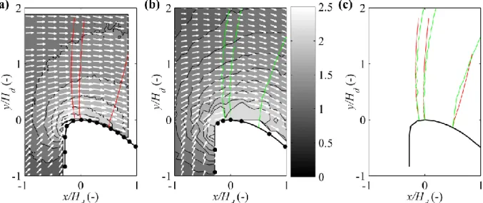
Figure 4. Contour plot of the norm of the velocity scaled by the discharge velocity, V, velocity fields and isopotentials evaluat-ed at three positions along the spillway (Black points = location of the pressure sensors). (a) W1, H/Hd = 5. (b) W2, H/Hd = 5.

(c) Superimposition of the computed isopotentials of W1 and W2.

The rotational of the velocity field was then computed for every flow-case. It was found weak except at some points in the flow, mostly close to the spurious vector locations. We therefore considered that the condition of irrotational flow was thus fulfilled in most part of the flow, which emphasizes that Equa-tion (8) should be a good approximaEqua-tion of the velocity evoluEqua-tion in the flow.

Thanks to the regularised least-square resolution previously described, the field of potential was com-puted and the velocity profiles along several isopotential lines were extracted from the velocity fields. The isopotentials are displayed in Figure 4 for three positions: x/Hd = -0.1, 0 and 0.5 along the spillway crest. The comparison of these lines for both spillway profiles in Figure 4(c) indicates that the

scaled-isopotential lines collapse well in most parts of the flow. As a consequence, the scaled-velocities taken along these isopotentials can also be compared for both spillways (Figure 5). In Figure 5, it results that for each position, the scaled-velocity distributions of both spillways are well collapsing, which indicates that no scale effect can be identified. Nevertheless, the curvature of the velocity profile close to the spill-way is slightly different. For W1, the latter is stronger and the scaled-velocity close to the bottom seems to be higher than for W2, which could indicate an acceleration effect close to the spillway.

Figure 5. Distribution along the isopotentials displayed in Figure 4 of the velocity v() normalized by the discharge velocity V.

3.2 Pressure

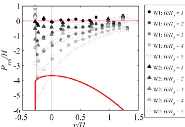
The relative pressure measured along the spillway centreline is plotted in Figure 6. It is normalised by the upstream head. While for the unity head ratio, the relative pressure along the spillway is close to zero (to the uncertainty), for higher head ratios, the relative pressure strongly decreases with increasing head ratio. In all cases, the minimum is measured upstream from the crest and the pressure then quickly increases to reach zero downstream from x = 1.5Hd for W2, while for W1 the last measurements quickly decrease. The position of the minimum pressure belongs to [-0.25Hd – -0.23Hd], which is consistent with the litera-ture (Melsheimer and Murphy 1970).

Figure 6. Relative pressure along the spillway crest

Similar behaviours are observed until H/Hd = 3 for W1 and W2, but for greater head ratio, ments of W1 are systematically smaller. This difference, which is coherent with the velocity measure-ments, could indicate a scale-effect, but can also be due to a measurement bias introduced by the size of the relative pressure sensor relatively to the size of the spillway. The surface of measurements is indeed larger for W2 than for W1, while it is clear that the minimal pressure is measured on a very limited length. Thus a larger surface averaging might occur in the case of W2.

4 DISCUSSION

As presented in the results’ section, the velocity fields when scaled by the appropriate variable emphasise a good adequacy between both cases for head-ratios equal or greater than two. In contrast, the relative

pressure measured along the spillway shows some discrepancies for head-ratios equal or greater than three. The full validation of the dataset therefore requires a method that puts into relation the pressure measurements and the velocity fields.

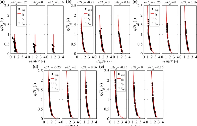
For each spillway, a least square optimisation was performed on Equation (8) in order to find the best couple {v0, r/|0} to fit the experimental velocities (r0 being fixed and deduced from the spillway ge-ometry). The velocity profiles for both spillways being close at a given head-ratio (Figure 4(c)), a mean fit per isopotential was then calculated. In Figure 7, the velocity profiles along three isopotentials are rep-resented together with the mean fit for W1. Similar results can be observed for W2 (not prep-resented here). For both spillway profiles, the mean fit and the experimental data are in good agreement, especially from

H/Hd ≥ 2, where the relative difference between the fit and the measurements are within ±5% and there-fore validates the use of Equation (8) so as the extrapolation of the velocities towards  = 0. Finally, by converting the relative pressure measured along the spillway crest into a velocity, v0p, using Equation (9) and z = zsensors, we can compare it to the fit of the velocity in  = 0 (i.e. v0) and validate or not the dataset.

Figure 7. Fit of the velocities taken along three isopotentials corresponding to measurement position of relative pressure along the spillway. (a) W1, H/Hd = 1. (b) W1, H/Hd = 2, (c) W1, H/Hd = 3, (d) W1, H/Hd = 4, (e) W1, H/Hd = 5.

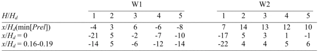
In Table 2, the relative difference between v0 and v0p is given for each spillway (v0 and v0p are also re-ported in Figure 7, see markers at Hd = 0). The velocity in  = 0, v0, is very close to the one computed from the relative pressure, v0p. Nevertheless trends appear between v0 and v0p. Except at H/Hd =1, when considering W1, the fit underestimates v0 with increasing head-ratio, while it overestimates it for W2, the influence of H/Hd being less clear. These results are still difficult to interpreted, as two antagonist phe-nomena seem to interact at the spillway. For W1 the evolution of the relative difference indicates a clear overestimation of the relative pressure amplitudes by the pressure sensor, which is consistent with the higher velocities observed for W1 (see in Figure 5). By contrast, for W2, the amplitudes of the relative pressure are clearly underestimated where the minimum relative pressure was found, while it is well measured in the other sections. This confirms that a spatial averaging might operate for the measurements of the smallest relative pressure.

Table 2. Relative difference in percent between v0 and v0p: (v0 – v0p)/v0p × 100 __________________________________________________________________________________ W1 W2 _________________________ _________________________ H/Hd 1 2 3 4 5 1 2 3 4 5 __________________________________________________________________________________ x/Hd(min[Prel]) -4 3 6 -6 -8 7 14 13 12 10 x/Hd = 0 -21 5 -2 -7 -10 -17 5 3 1 -1 x/Hd = 0.16-0.19 -14 5 -6 -12 -14 -22 4 4 5 6 __________________________________________________________________________________ 5 CONCLUSION

Experiments on two identical ogee spillways at different scales were conducted for heads largely greater than the design head. The aim of this paper is to validate velocity and relative pressure measurements.

The velocity fields were measured by LSPIV. Most of the spurious data were identified close to the spillway and some differences between both spillways are observed in this area. For the greater spillway, the relative flow velocity is indeed slightly higher. In the rest of the field, the data are in good agreement for both configurations from a head ratio of two.

The relative pressure along the spillway was measured using relative pressure sensors of small size. Measurements are coherent between both configurations until a head ratio of three. Above this head-ratio, a smaller relative pressure is measured for the larger spillway, which corroborates the velocity measure-ments.

The difference between both spillway profiles in term of relative pressure is finally discussed using a theoretical fit of the velocity fields, based on the theory of potential flows. For this theory, the fitting re-quires the identification of the potential field, because it operates on velocities that belong to the same isopotential. The relative pressures along the spillway crest, converted into velocities using Bernoulli’s equation, are compared to the fit of the velocity until the spillway crest. Results confirm that amplitudes of relative pressure are overestimated for the larger spillway, while an averaging effect due to the size of the sensor is present for the smaller spillway.

ACKNOWLEDGMENTS

The authors are grateful for the physical model preparation by the laboratory technicians of HECE and the fruitful discussions about spillway flows with F. Stilmant (HECE), B. Blancher (EDF–CIH), J. Ver-meulen (EDF–CIH) and D. Aelbrecht (EDF–CIH).

This work was partly supported by Electricité de France – Centre d’Ingénierie Hydraulique (EDF– CIH), Order 59101012800 PIAT 037.

NOTATION

A gradient matrix expressed in finite differences (m-1₎

B width of the spillway (m)

h water depth above the spillway-crest measured at x = xm (m)

h uncertainty on the water depth (m)

huf height of the upstream face of the spillway (m)

g gravity acceleration (m.s-_²)

H head (m)

H uncertainty on the head (m) Hd design head (m)

Hmax design maximal head (m)

Prel relative pressure (m)

P uncertainty on the pressure (m) Q discharge at the inlet (m³.s-1₎

Q uncertainty on the discharge (L.s-1₎

r0 curvature radius when h0 = 0 (m)

r curvature radius (m)

r0 curvature radius when h0 = 0 (m)

u longitudinal component of the velocity (m.s-1₎

w vertical component of the velocity (m.s-1₎

v norm of the velocity (m.s-1₎

v0 norm of the velocity in 0 (m.s-1)

v0p norm of the velocity in 0 computed from the relative pressure measured on the spillway (m.s-1)

x streamwise direction (m)

xm streamwise position of the measurement section (m)

y spanwise direction (m) z vertical direction (m)

 curvilinear coordinate along a streamline (m)  curvilinear coordinate along an isopotential line (m)

0 origine of the curvilinear coordinate along an isopotential line (m)

 potential (m².s-1₎

 local direction of the flow in the curvilinear reference frame (rad)  volume mass of water (kg.m-_³)

REFERENCES

Abecasis, F.M. (1970). Discussion of "Designing Spillway Crests for High-Head Operation" by Cassidy. J. Hydraulics Divi-sion, Vol. 96, No. 12, pp. 2654–2658.

Cassidy, J.J. (1970). Designing Spillway Crests for High-Head Operation.J. Hydraulics Division, Vol. 96, No. 3, pp. 745–753. Castro-Orgaz, O.(2008). Curvilinear Flow over Round-Crested Weirs. J. Hydraulic Res., Vol. 46, pp. 543–547.

Hager, W.H. (1987). Continuous Crest Profile for Standard Spillway. J. Hydraulic Eng, Vol. 113, No. 11, pp. 1453–1457. Hauet, A. (2009). Discharge Estimate and Velocity Measurement in River Using Large Scale Particle Image Velocimetry. La

HouilleBlanche, No. 1, pp. 80–85.

Hauet, A., Creutin, J.D. and Belleudy, P. (2008a). A Sensitivity Study of Large-Scale Particle Image Velocimetry: Measure-ment of River Discharge Using Numerical Simulation. J. Hydrology, Vol. 349, No. 1-2, pp. 178–190.

Hauet, A., Kruger, A., Krajewski, W.F., Bradley, A., Muste, M., Creutin, J.D. and Wilson, M. (2008b). Experimental System for Real-Time Discharge Estimation Using an Image Based Method. J. Hydrologic Eng., Vol. 13, No. 2, pp. 105–110. Melsheimer, E.S., and Murphy, T.E. (1970). Investigations of Various Shapes of the Upstream Quadrant of the Crest of a High

Spillway. U.S. Army Corps of Engineers, Waterways Experiment Station, Vicksburg, Mississippi, USA.

Millet, J. C., Chambon, J. Soyer, G. and Lefevre, C. (1988). Augmentation de la Capacité des Ouvrages d’Evacuation de Di-vers Barrages. 16ème Congrès Des Grands Barrages, SanFrancisco, USA, 13–17 June 1988.

Oertel, H. 2010. Prandtl-Essentials Fluid Mechanics. Springer New-York, 790 pages.

Reese, A.J., and Maynord, S.T. (1987). Design of Spillway Crests. J. Hydraulic Eng. Vol. 113, No. 4, pp. 476–490. Rouse, H., and Reid, L. (1935). Model Research on Spillway Crests. Civil Eng., ASCE, Vol. 5, No. 1, pp. 10–14.

USACE. (1987). Hydraulic Design Criteria. U.S. Army Corps of Engineers, Waterways Experiment Station, Vicksburg, Mis-sissippi, USA.

USBR. (1948). Boulder Canyon Project. Final report. Studies of Crests for Overfall Dams. U.S. Department of Interior, Den-ver, CO, USA.

USBR. (1987). Design of Small Dams. U.S. Department of Interior, Denver, CO, USA.

Vermeyen, T.B. (1991). Hydraulic Model Study of Ritschard Dam Spillways. U.S. Department of Interior, Denver, CO, USA. http://www.usbr.gov/pmts/hydraulics_lab/reportsdb/wrrl_reports_action2.cfm?id=R-91-08.

Vermeyen, T.B. (1992). Uncontrolled Ogee Crest Research. http://www.usbr.gov/pmts/hydraulics_lab/pubs/PAP/PAP-0609.pdf.

Westerweel, J.A. and Scarano, F.B. (2005). Universal Outlier Detection for PIV data. Exp. Fluids, Vol. 39, No. 6, pp. 1096– 1100.

Xlyang, J. and Cederström, M. (2007). Modification of Spillways for Higher Discharge Capacity. J. Hydraulic Res., Vol. 45, No. 5, pp. 701–709.