Adaption to auditory localized cues from an enlarged head

(1)

Adaptation to Auditory Localization Cues

from an Enlarged Head

by

Salim Kassem

B.S., Electrical Engineering (1996) Pontificia Universidad Javeriana

Submitted to the Department of Electrical Engineering and Computer Science in Partial Fulfillment of the Requirements for the Degree of

Master of Science in Electrical Engineering and Computer Science

at the

Massachusetts Institute of Technology

June 1998

Signature of Author ... ... ...

Department of Electrical Engineering and Computer Science May 20, 1998

Certified by ...

Nathaniel I. Durlach Senior Research Scientist of Electrical Engineering and Computer Science

- /Thes Supervisor

Accepted by ... ...rthu C.Sm th

AccptembyArthur C. Smith

Chairman, Department Committee on Graduate Students gra Se%94i~iA

(2)

Adaptation to Auditory Localization Cues

from an Enlarged Head

by

Salim Kassem

Submitted to the Department of Electrical Engineering and Computer Science on May 20, 1998 in Partial Fulfillment of the Requirements for the Degree of

Master of Science in Electrical Engineering and Computer Science

ABSTRACT

Auditory localization cues for a double-size head were simulated using an auditory virtual environment where the acoustic cues were presented to subjects through headphones. The goals of the study were to see if better-than-normal resolution could be achieved and analyze how subjects adapt to this type of transformation of spatial acoustic cues. This worked follows that done by Cunningham (1994, 1998) and Shinn-Cunningham, Durlach and Held (1998a, 1998b), where a nonlinear remapping of the normal space filters was implemented. The double-size head's acoustic cues were simulated by frequency-scaling normal Head Related Transfer Functions. As a result, the Interaural Time Differences (ITDs) presented for every position were doubled. Therefore, even though the relationship between the location a naive listener associates with a stimulus and its correct location is not linear, it is a linear transformation in ITD space. Since ITDs were doubled, some ITDs presented to the listener were larger than the largest naturally-occurring ITDs, which proved to be a problem. Bias and resolution were the two quantitative measures used to study performance as well as to examine changes in performance over time. Also, the Minimum Audible Angles for normal and altered cues were determined and used to obtain estimates of subjects' sensitivity.

In the experiments, mean response and bias changed over time as expected, clearly showing the adaptation process. Resolution results were less consistent, giving better-than-normal resolution around the middle positions with altered cues. Nevertheless, normal cues provided better overall performance. When correct-answer feedback was used, resolution behaved as expected, but when feedback was not presented, results were consistent with subjects attending to the whole range of possible cues throughout the experiment (i.e., the internal noise was large and constant). Previous work suggested that mean response, bias and resolution are dependent on each other and that all have the same adaptation rate. However, the no-feedback condition proved that resolution can be independent of the other quantities.

Finally, estimates of sensitivity indicated that resolution is strongly related to the type of cues used and that changes in resolution depend directly on the total internal noise.

Thesis Supervisor: Nathaniel I. Durlach

(3)

ACKNOWLEDGMENTS

Dedico este trabajo de grado a mi esposa, quien me di6 todo el apoyo, toda la amistad y todo el amor que necesitd. Gracias por creer en mi.

A mis padres y hermanos, por ayudarme a ser como hoy soy. A mi papa', porque sin su esfuerzo no podria estar aquf.

A mis verdaderos amigos.

This work is dedicated to my wife , who support, all the friendship and all the love you for believing in me.

gave me all the

I needed. Thank

To my parents and siblings, for helping me be who I am. To my father; without his effort I would not be here.

To my truly good friends.

I want to thank Nathaniel Durlach for his support and for giving me the opportunity of learning wonderful things.

Special thanks to Barbara Shinn-Cunningham, for all her unconditional help. Without her guidance, this work could never have been finished.

I also want to thank Lorraine Delhorne, Jay Desloge and Andy Brughera for all their kind collaboration.

(4)

1. INTRODUCTION

In recent years, computing technology has provided us with more sophisticated ways of gathering data, increasing the amount and complexity of the information presented to users. As a result, the systems that work with this information are more complex and more difficult to operate and understand. Today's graphic computer interfaces are a first approach to easing the resulting burden of displaying information. Lately, attention has been given to a more sophisticated interface, referred to as virtual reality, whose objective is to provide a more efficient and natural way of presenting and manipulating information by incorporating a three-dimensional spatial cues in the display (Wenzel, 1992).

Using this technology, a human operator can interact with a real environment via a human-machine interface and a telerobot as if he were the one standing in the remote working area. Ideally, the operator should see, hear, and feel what the telerobot sees, hears, and feels. Moreover, the telerobot can provide additional information that can be useful to the operator (e.g., temperature, speed, etc.). Normally, the teleoperator system is used to interact with a remote, inaccessible or hazardous environment, protecting the physical integrity of the operator while permitting him to control and achieve a specific task. The signals in the telerobot's environment are sensed, sent back, and displayed to the human operator. In the same way, the actions taken by the operator in response to the signals are transmitted to the telerobot and used to control its actions (Durlach, 1991).

In a virtual-environment system, the same kind of human-machine interface is used, but a computer simulation replaces the telerobot and the environment. The purpose of a teleoperator system is to extend the operator's sensory-motor system in order to facilitate the manipulation of the physical environment, while in a virtual reality system the objective is to study or alter the human operator. General information on teleoperators and virtual-environments can be found in Vertut and Coiffet (1986), Sheridan (1987), Bolt (1984), Foley (1987), and Durlach and Mavor (1995).

(7)

In the past, use of the visual modality was the primary method for presenting spatial information to a human operator. However, more recently, the auditory system has become recognized as an alternative for delivering such information. Acoustic signals are very useful because they can be heard from any source direction, they tend to produce an alerting or orienting response, and they can be detected faster than visual signals (Wenzel, 1992). In this project, attention is given only to the auditory localization features of the machine-human interface, and particular consideration is given to how to provide the operator with a better-than-normal localization ability, so-called supernormal auditory localization (Durlach, Shinn-Cunningham, and Held, 1993). Such an approach attempts to provide acoustic cues that yield better effective spatial resolution than do normal cues. This is achieved by increasing the change in the physical acoustic cues that result when source position changes. Improving the effective resolution is desirable because the normal human auditory localization system has extremely poor resolution in azimuth at angles off the side, in elevation, and in distance; it has at least a moderate resolution only in azimuth for sources in the front. In other words, we have relatively poor spatial resolution for acoustic sources, especially when compared with visual spatial resolution.

Durlach, Shinn-Cunningham, and Held (1993) proposed several ways to increase the directional resolution by using localization cues that would improve the just-noticeable-difference (JND) (i.e., the minimum separation for which a listener can resolve two adjacent spatial positions). Some of the suggested methods for achieving supernormal cues include simulating the localization cues from an enlarged head, remapping the normal localization cues to increase resolution in some regions of the azimuth plane while decreasing it in others, and exponentiating the complex interaural ratio at all frequencies (Durlach and Pang, 1986). As Shinn-Cunningham (1998a) noted, these approaches should improve the subject's ability to resolve sources in JND-type experiments, but the effects on identification tasks using a larger range of physical stimuli are not clear. In addition, the use of supernormal localization cues will displace the apparent location of the source for a naive listener when he is first exposed to these remapped cues. Adaptation to the new cues is said to have taken place to the extent that the mean localization error diminishes over time with training.

(8)

Given the results obtained in a previous work by Shinn-Cunningham (1994) and Shinn-Cunningham, Durlach and Held (1998a, 1998b), a study of supernormal auditory localization cues will be undertaken, using the suggested enlarged head approach (Durlach, Shinn-Cunningham, and Held, 1993). Auditory localization cues for a double-sized head will be simulated and presented to the subjects during the experiments. The main goals of this project will be: To analyze how subjects adapt to a transformation of spatial acoustic cues that is approximately linear, to extend the quantitative model of adaptation developed from the nonlinear adaptation results (Shinn-Cunningham, 1998), and to see if better-than-normal resolution is achieved with the double-head size cues. Also, the results of this experiment will be compared with those of Shinn-Cunningham (1994 and 1998) and Shinn-Cunningham, Durlach and Held (1998a, 1998b) to explore how different types of remappings affect adaptation to remapped auditory spatial cues. Following their work, bias (a measure of response error in units of standard deviation) and resolution (the ability of reliably differentiate between nearby stimulus locations) are the two quantitative measures that will be used to analyze the performance of subjects over the course of the experiments.

(9)

2. BACKGROUND

2.1. Normal Auditory Localization

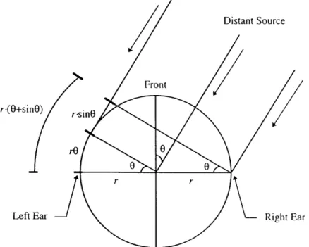
The classic duplex theory (Lord Rayleigh, 1907) states that the interaural differences in time of arrival and interaural differences in intensity, are the two primary cues used for auditory localization (Figure 1). Interaural time differences (ITDs) arise when a sound source is to one side of the head, since the sound reaches the nearest ear first'. If a sound source is far enough from the head, then sounds' wavefront is approximately planar when it reaches the head. The distance the sound must travel to reach the two ears differs, depending on source location. Assuming a spherical model of the head with radius r, the difference in the travel distance for a source on the horizontal plane at an angle of 0 (in radians) is given by (Figure 2):

Ad = r -(0 + sinO). (1)

Assigning a radius of 8.75 cm to the spherical head, and knowing that the velocity of sound c is 343 m/sec, the interaural time difference (ITD) can be expressed as:

ITD Ad 255x 10-6 -(0 + sin0) [sec]. (2)

C

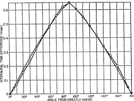
Figure 3 shows predictions of ITD based on equation 2 and measurement of ITD for adult males (Mills, 1972).

The duplex theory states that the relative left-right position of a sound source is determined by ITDs for low frequency sounds and IIDs for high frequency sounds. As the duplex theory explains, ITDs give good perceptual cues for sound location only for low

The sound will reach the farther ear 29 psec later per each additional centimeter it must travel (Mills,

(10)

frequencies; at frequencies higher than 1500Hz, phase ambiguities occur. The phase information becomes ambiguous at high frequencies because the wavelengths are smaller than the distance between the ears.

closer

Interaural sources off

sooner at t

--- -- IID

closer ear Interaural Intensity Differences (lIDs):

sources off to one side are louder at the closer ear due to head- shodowing

Figure 1. The duplex theory postulates that interaural intensity differences (lIDs) and interaural time

differences (ITDs) are the two primary cues for auditory localization (from Wenzel, 1992).

r-(O+si

Lef

Figure 2. Differences between the distances of the ears from a sound source that is far away and that can be represented as a plane wave front (from Mills, 1972).

(11)

On the other hand, sources off to one side of the head are louder at the closer ear due to head-shadowing; the head acts as a low-pass filter for the far ear, making IDs

important localization cues for high frequencies. This acoustic effect occurs because wavelengths are large relative to the size of the head at high frequencies.

It has been found that ITD is the major cue for determining the location of sources along the horizontal plane, and that the spectral peaks and the notches produced by the filtering effect of the pinnae (mainly above 5kHz) are important for determining source elevation.

Even though the duplex theory provides a clean and simple explanation for determining the lateral position of a sound, this approach presents several limitations. For example, listeners use the time delay envelope of high frequency sounds for localization even though they do not use ITD at these frequencies. The direction-dependent filtering that occurs when sound waves impinge on the outer ears and pinnae also provides very important localization cues. It has been shown that the spectral shaping by the pinnae is highly directional dependent (Shaw, 1974 and 1975), and that the pinnae is responsible for the externalization of the sounds (Plenge, 1974).

ANGLE FROM DIRECTLY AHEAD

Figure 3. Interaural time difference (ITD) as a function of the position of a source of clicks. X: measured values from five subjects. 0: values computed from the mathematical approximation (from Mills, 1972).

(12)

0-Therefore, the auditory system's method for determining source position depends on a directional dependent filtering that occurs when the received wave sound interacts with the head, ears, and torso of the listener. Let X(w) be the complex spectrum of the sound source and YL(m,O,B) and YR(Wm,O, ) be the complex spectrum of the signals received in the left and right ear respectively. Then, for sources that are sufficiently far from the listener (so that distance only affects the overall level of the received signals), and for anechoic listening conditions, one can write:

YL(O, 0,) = r-' -HL(o,, ) -X(o) (3a)

Y, (o,,) = r -' HR (0,0,) • X(O), (3b)

where r is the distance from the head to the source, and HL(o,,,) and HR(m,0,4) are the space filters or Head Related Transfer Functions (HRTFs) for each ear, describing the directional dependent effects of the head and body. The HRTFs depend on the frequency, o; the azimuth of the sound source relative to the head, 0; and the elevation of the source relative to the head, 0.

The auditory system compares the signals received at the two ears in a manner that can be usefully represented mathematically by forming the ratio:

YL(o,)0,) HL(O,0',) (4)

YR (W,O, ) HR (,0,0)

In this ratio, the effect of r and the effect of X(w) are canceled, and the ratio depends only on o, 0, and 0. The auditory system can determine the location of the sound source from the ratio, independent of source characteristics. The magnitude and the phase of the ratio of the signals at the two ears for a source at direction (0,0) are equivalent to the interaural intensity difference (IID) and the interaural time difference (ITD), respectively.

Even though interaural processing (i.e., computation of IID and ITD) offers useful localization information, directional ambiguities can occur: (i) distance is not perceived because its effect is negligible for distant sources, and (ii) front-back confusions appear

(13)

because of the so-called cone of confusion2 _{(Mills, 1972). Head movements and monaural}

processing help to resolve front-back ambiguities. Head movements cause changes in IID and ITD which differ for a source in front or behind the listener. Also, a priori knowledge or information about the transmitted signal X(o) can allow monaural spectral cues to be used to estimate the space filters HL(o,O, ) and HR(o,O,) from the signals YL(0,0,0) and YR(w,O,) received at the two ears.

Wightman and Kistler (1992) found that low-frequency ITDs are the dominant cues for localization of broadband sound sources. Although ITD cues are dominant, when the low-frequency components of a stimulus are removed, direction is determined by IID and spectral shape cues. In other words, when low-frequency interaural time cues are present, they override the ID and the spectral shape cues that are present in other frequency ranges. It follows that in every condition in which there is a conflict between low-frequency ITD and any other cue, sound localization is determined mainly by ITD.

The ITD is used primarily to establish the locus of possible source location (i.e., to determine on which cone of confusion the sound source lies), while lID and spectral filtering help to resolve any ambiguity in ITD information. Integration of all available cues leads to accurate localization (Wightman and Kistler, 1992).

More information about normal auditory localization can be found in Blauert (1983), Mills (1972), Wightman, Kistler, and Perkins (1987), Wenzel (1992) and Durlach, Shinn-Cunningham and Held (1993).

2.2. Auditory Virtual Environments

In order to better understand the importance of auditory cues such as ITD, IID and pinnae effects, and to enhance their capabilities, researchers have begun to use auditory virtual environments to simulate acoustic sources around the listeners. This approach

2 _{The cone of confusion errors arise because a given ITD or IID produced from one source position is}

roughly equal to that produced by sound sources located at any place over the surface of a hyperbolic surface (with a cone shape) whose axis is the interaural axis.

(14)

gives the experimenter good control of the stimulus while creating rich and realistic localization cues.

One class of simulation technique derives from the measurement of Head Related Transform Functions (HRTFs). Using a normative mannequin, such as the KEMAR (Knowles Electronics, Inc.), it is possible to obtain good estimates of the acoustic effects of the head and the pinnae on sounds reaching the listeners' ear drum as a function of source position. Using these finite impulse response (FIR) filters, it is possible to filter an arbitrary sound to give it spatial characteristics (i.e., to simulate a sound coming from a predetermined direction). Even though the HRTFs provide good acoustic cues, the localizability of the sound also depends on other factors, such as its original spectral content (e.g., narrow band sounds like pure tones are harder to localize than broad band tones). Individual differences in the pinnae appear to be very important for some aspects of localization, most notably resolving cone of confusion errors. Several studies show that most listeners can obtain useful directional information from a typical HRTF, suggesting that the basic properties of the HRTFs carry much of the important localization information (Wenzel, 1992).

Using digital signal processing (DSP) systems, real time simulation of acoustic cues can be used to generate spatial auditory cues over headphones. These systems use time domain convolution to achieve the desired real time performance, reproducing a free-field experience. Using a head tracker device attached to the headphones, the system can determine the actual head's yaw, pitch and roll and decide which set of HRTFs is needed for presenting a source from a particular position. The DSP system will then filter the input signal with the proper HRTF. Even if the subject's head is moving freely, the head tracker allows the presentation of a fixed sound location by calculating the relative azimuth and elevation from the source to the head. Of course, the term real time is a relative one given that it is not possible to select the appropriate HRTF on the fly. Some processing time is needed for all the computations. Due to the constraints of memory and computation time, DSP systems must make several approximations and simplifications, losing some reliability.

(15)

A typical HRTF record consists of a pair of impulse responses (i.e., one for the right and one for the left ear), measured from several equidistant locations around the subject. The HRTFs are then estimated by canceling the effects of the loud speakers, the stimulus, and the microphone responses from the recorded signal (Wightman and Kistler, 1.989). For example, the HRTFs measured by Wightman and Kistler (1989) from their subject SOS consisted of 36 azimuth positions (with a 100 resolution) ranging from 1800 to -170', and 14 elevation positions (with a 100 resolution), ranging between 80 to -500. Hence, the HRTFs represented a total of 504 positions (36 in azimuth times 14 in elevation). The HRTF for a specific position is stored as two 127 tap FIR filters, each containing the impulse response for one of the ears.

Figure 4 shows typical HRTF waveforms for two different locations in azimuth at

0' elevation, and demonstrates how ITD and IID vary as a function of the direction of the

sound source. For a source at 0O in azimuth (i.e., right in front of the listener), there is very little difference in either the magnitude (lID) or the phase (ITD) responses for both ears (top right plots); this is highlighted by taking the ratio between the responses of both ears (bottom right plots). Because sound arrives almost at the same time and with the same magnitude at both ears, the ratio of the phase and magnitude is almost zero. For a source at -400 in azimuth (i.e., to the left of the listener), the magnitude (lID) of the left ear is greater than the one of the right, while the phase (ITD) of the right ear is larger (top

left plots). As expected, the ratio between the right and left ear responses (bottom left plots) shows a negative magnitude (i.e., the sound at the right ear has less energy than the sound at the left ear) and a negative overall phase (i.e., the sound arrives at the right ear later that at the left ear).

2.3. Sensory Improvement

It is now possible to think not only of better ways to simulate normal localization cues, but also of methods for transforming the natural acoustic cues for the purpose of achieving better spatial resolution (e.g., superlocalization, Durlach, 1991).

(16)

Frequency response left(-) and right(- -- ) ear (40 degrees)

100 80

I s

1 000 400 MXX 800 10 12 0

70 Jr-- Frequency response righf/teft -' ear (40 degrees)

20 -10 40L 0 2000 4000 6000 8000 10000 12000 0 20 -30 -60--80 -1001 0 2000 4000 6000 8000 10000 12000 Frequency (HzJ

Frequency response rightWlf eer (-40 degrees) 20 10 0 -10- -20--30 -401 0 2000 4000 6000 8000 10000 12000 10 0 -10 20-30 -401 0 2000 4000 6000 8000 10000 12000 Frequency 1Hzl

Frequency response let(--) and right(- - -) ear (0 degrees)

10 -90 0 6000 8 10 12 70 if 60 0 -20 -40 -60--100 0 2000 4000 6000 8000 10000 12000 -10- -20-0 2000 4000 6000 8000 10000 12000 0 to -20 -30 -40 0 2000 4000 6000 8000 10000 12000 Frequency (HzJ

Figure 4. Frequency responses for -40o and 00 in azimuth and 0' in elevation of the HRTFs measured by Wightman and Kistler (1989) from their subject SOS. The figure illustrates how the HRTFs contain the IID, ITD, and pinnae effect cues.

Some studies have tried to show how subjects adapt to unnatural auditory localization cues. One set of such studies (Warren and Strelow, 1984; Strelow and Warren, 1985) investigated the use of the Binaural Sensory Aid, a device that used auditory localization cues as a way of representing the position of objects sensed with sonar. Here, the ITDs contained information about the distance from the object, and the IIDs gave its direction. The results of this study showed that blindfolded subjects were able to adapt and use these unnatural cues accurately, after being trained using a correct-answer feedback paradigm.

In an attempt to improve spatial resolution (i.e., improving the JND in direction), a study on supernormal auditory localization was undertaken (Durlach, Shinn-Cunningham, and Held, 1993). Its main goal was to determine if adaptation to rearranged

(17)

In this study, supernormal localization cues were created by remapping the relationship between source position and the normal HRTFs (Durlach, Shinn-Cunningham, and Held, 1993). The transformation was supernormal only for some positions. At other positions the rearrangement actually reduced the change in acoustic cues with changes in source location. To simulate a sound at position 0, the study used HRTFs that were chosen from the normal HRTF set, but which normally correspond to a different azimuth. The new HRTFs are given by:

H'(w, 0, ) = H(o, f, (),). ₍₅₎

'With this transformation no new HRTFs were created. Instead, the existing HRTFs were reassigned to different angles.

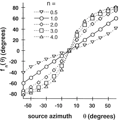
The family of mapping functions fo(O) used to transform the horizontal plane was given by:

(0) I tan 1- 2 2n sin(20) (6)

2 1-n2 _{+(I+n')cos(26)}

where the parameter n gives the slope of the transformation at 0=0°. Figure 5 shows this transformation for several cases of n. When n=l, cues are not rearranged. With n>l the transformation increased the cue differences (and therefore the resolution) around values of 0=00, while it decreased them in the neighborhood of 6--90. For n<l the opposite occurred. As a result, subjects were expected to show better-than-normal resolution in the

front, and lower resolution towards the sides when n>1.

In the study, subjects were first tested with normal localization cues (to determine baseline performance), and then with altered (supernormal) cues to examine how performance changed with training. Finally, normal cues were presented again to see if there was any after-effect as a result of training.

Bias, a measure of the error in the subjects response, and resolution, a measure of the ability to resolve adjacent stimulus positions, were the two quantities used to analyze

(18)

the adaptation process throughout the experiments. Figure 6 and 7 illustrates bias and resolution results for one of the experiments in this study, in which correct-answer feedback was used to train the subjects.

Co a)3 1.. 0) a) *0 80 60 40 20 0 -20 -40 -60 -80 -50 -30

source

V. -10

azimuth

10 30 50 0

(degrees)

Figure 5. A plot of the azimuth remapping transformation specified by equation 6 (from

Shinn-Cunningham, Durlach, and Held, 1998a).

The first normal cues are expected to show small bias (error in units of standard deviation) since cues are roughly consistent with normal localization cues. The first run using altered cues resulted in a very large bias, indicating the sudden introduction of the unnatural sounds. The last run using altered cues showed a decrease in bias compared to before training, demonstrating that the correct answer feedback caused subjects to adapt

to the new cues (although, adaptation was not complete). Finally, the first normal cue test following training with altered cues produced a negative after-effect, indicating that the performance was not controlled exclusively by conscious correction (Shinn-Cunningham, Durlach, and Held, 1998a).

Resolution of adjacent source locations is shown in Figure 7. In the first normal cue run, resolution provides a standard against which other results are compared. As

(19)

expected, when altered cues were presented for the first time, resolution increased around the center positions and decreased at the edges of the range. In the last run with altered cues, resolution remained enhanced (with respect to the baseline), but showed a decrease compared to the first altered cue run. As before, an after-effect was seen after normal cues were introduced again (Shinn-Cunningham, Durlach, and Held, 1998a).

- -- - n=1

2.41.6 -

0.8Pi 0.0

-

-0.8-

-1.6-

-2.4-- - - -- n=3 - n=3 o-- - n= 9 O- ₀ o~ Io

-60 -40 -20

0 20 40 60

Source position (degrees)

Figure 6. Bias results for one of the experiments carried out. 0: First run in the experiment using normal cues. ': First run with altered cues. *: Last run with altered cues. 0: First normal cue run following altered cue exposure. Here, the altered cues have a transformation strength of n=3 (from Shinn-Cunningham, Durlach, and Held, 1998a).

This study showed that subjects could not adapt completely to a nonlinear remapping of the auditory localization cues. In general, subjects were able to reduce their response bias with training, but they could never completely overcome their errors. In addition, although the transformation initially increased resolution as expected, resolution decreased as subjects adapted to the remapping. Shinn-Cunningham, Durlach and Held (1998a) concluded that resolution depended not only on the range of physical cues presented during an experiment, a result previously described for perception of sound intensity (e.g., Durlach and Braida, 1969; Braida and Durlach, 1972), but also upon the past history of exposure or training of the subject. The researchers also found that

(20)

subjects adapted to the best-fit linear approximation of the nonlinear transformation, implying that subjects may only be capable of adapting to linear transformations of the localization cues (Shinn-Cunningham, Durlach and Held, 1998b).

4.0

3.0 d'

i

2.0

1.0

0.0 -60 -40 -20

0

20

40

60 Source position (degrees)

Figure 7. Resolution results for one of the experiments carried out. 0: First run in the experiment using normal cues. +: First run with altered cues. *: Last run with altered cues. 0: First normal cue run following altered cue exposure. Here, the altered cues have a transformation strength of n=3 (from Shinn-Cunningham, Durlach, and Held, 1998a).

(21)

3. ADAPTATION TO SUPERNORMAL CUES

3.1. Motivation

The main goal of this project is to examine further whether humans can adapt to unnatural (altered) auditory localization cues that will provide listeners with better-than-normal localization ability, so-called superbetter-than-normal auditory localization (Durlach, Shinn-Cunningham, and Held, 1993).

In contrast with the previous study Listed above (e.g., Shinn-Cunningham et al., 1994 and 1998) where a nonlinear remapping of the normal space filters was implemented, a more linear approach that expands all positions is now taken to create supernormal HRTFs. The earlier experiments showed that subjects adapted to the best-fit linear approximation of a nonlinear transformation. This could mean that subjects are only able to adapt to linear transformations. This study is designed to give further insight into the adaptation process to determine if this linear constraint holds for other cue transformations. In addition, the new transformation may provide listeners with a higher spatial sensitivity and, hopefully, a low overall localization error.

3.2. Supernormal Auditory Localization: Double-Size Head

To improve resolution, the localization cues must increase the discriminability between separated sources. This may be achieved by having a larger-than-normal difference in the physical cues corresponding to two different positions. One way of achieving this is by simulating a larger-than-normal head, thereby increasing the ITDs and lIDs associated with every position in space. For a subject who has not adapted to such a change in cues, the use of such a transformation will make him think that the location of sound sources are farther apart than they actually are.

(22)

The double-size head was simulated by frequency scaling normal HRTFs (Rabinowitz, Maxwell, Shao, and Wei, 1993). The new pair of HRTF filters are defined as follows:

HL (0,,4) = HL(K(o,,)

R (o0,8,) = HR (Ko,,4), (7)

where K has a constant value. This transformation approximates the acoustic effect of increasing the size of the human body, including the head and pinnae, by a factor of K. As a result, the IlD and ITD will also be affected, and will be determined by the new ratio:

1 (8)

YR (,0,) HR (0)O,)

Here, both the interaural differences and the monaural spectral cues are magnified by the factor K (Durlach, Shinn-Cunningham, and Held, 1993), and therefore, it is said to be a linear transformation. For the current study, the frequency was doubled (i.e., by setting K=2), simulating a head twice the normal size. As Rabinowitz, Maxwell, Shao, and Wei (1993) showed, scaling the HRTFs corresponds to uniformly scaling up all physical dimensions to simulate the main acoustic effects of a magnified head.

The transformation of the HRTFs presents several problems: Scaling the frequency of the normal HRTFs can be achieved by inserting an additional sample equal to zero after each sample of the original HRTF impulse response. This causes the time signal (i.e., the impulse response) to increase in length by a factor of two (i.e., K=2). In the frequency domain, the spectrum is compressed by a factor of two. The new HRTFs must be low-pass filtered to remove energy above the original Nyquist frequency. For example, if the normal HRTFs are defined up to 20kHz, the new HRTFs are only defined up to 10kHz. Without low-pass filtering the upsampled waveforms, this procedure would create distortion of the spectrum above 0lkHz due to spectral aliasing.

(23)

Conversely, since the size of the head is doubled, the ITDs presented to the listener will include larger ITDs than the largest naturally-occurring ITDs. For example, a source at 900 (or -900) will produce the maximum normal ITD of around 0.65 msec (Figure 3). With the transformed cues, the corresponding ITD will be 1.3 msec. It is not clear how subjects will perceive these unnatural cues. As a consequence, subjects must adapt to the expanded interaural axis not only by relabeling it, but also by interpreting larger than normal ITDs (Durlach, 1991).

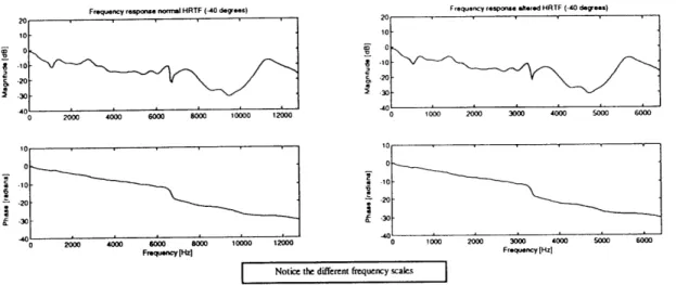
Normal HRTFs from subject SOS (Wightman's and Kistler's, 1989) were used to create the double-head HRTFs. Each position described by the HRTFs contains two 127 tap FIR filters (one containing the filter coefficients for the right ear and one for the left ear) sampled at 50kHz. To create the double-head HRTFs, each FIR filter was upsampled by a factor of two and then low pass filtered at 25kHz (Figure 8). As a result, the new altered HRTFs were two times longer (i.e., each FIR filter is now 254 tap long), and sampled at 100kHz.

Frequency response normal HRTF (40 degrees) Frequency response altered HATF (-40 degrees)

-10 -100 2000 00 3000 4000 5000 60 -40 -400 0 2000 4000 000 000 10000 102000 1000 2000 3000 4000 5000 6000 0 0 Frequency [Hz] Frequency (Hz]

Notice the different frequency scales

Figure 8. Comparison between normal and altered HRTFs for a source at -400 in azimuth. The left panel shows the normal HRTF while the right one shows the altered HRTF under different frequency scales. The shapes of both frequency responses are the same, except for the fact that the altered HRTF has been scaled in frequency, indicating that the upsampling was successful. Note that the ITD (given by the slope of the phase as a function of frequency) for the altered HRTF is now doubled.

Figure 8 compares the frequency responses of the HRTF at -400, showing that the upsampling doubles the ITD (the ITD is given by the slope of the phase response as a function of frequency). As mentioned above, the altered HRTFs are now compressed in

(24)

frequency by a factor of two, and in order to prevent unpredictable results at high frequencies, the new HRTFs were low-pass filtered. As a result, the magnitude response is effectively zero above 12.5kHz..

3.3. Equipment and Experimental Setup

Adaptation to the double-size head auditory localization cues was investigated by presenting simulated acoustic cues and real visual cues. The acoustic cues were generated by an auditory virtual environment. Visual cues were provided by a light display located in front of the subjects. The visual cues were used to provide the subjects

with spatial feedback about the simulated sounds.

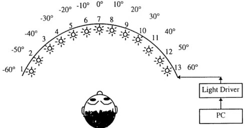
Subjects were seated in front of a five-foot-diameter arc of lights, consisting of thirteen 2 inch light bulbs. The lights were labeled from 1 to 13 (all lights were visible to the subjects during the experiment). The lights were positioned from -600 to +600 in azimuth with respect to the head position, with a 100 separation between each pair of lights. The position -60o azimuth was represented by light 1, 0O by light 7, 60' by light 13, etc. The light array was connected to a digital-analog device, the light driver, which receives a digital input from a personal computer (PC) and converts it to an analog output that drives the current to each light bulb. The PC used Data Translation's DT2817 Digital I/0 Board to transmit signals to the light driver, enabling it to turn the light on or off at any of the 13 positions (Figure 9). This light array provided visual feedback to the subjects.

The acoustic cues were simulated by an auditory virtual environment system consisting of a PC, a signal-processing device, a head tracker, headphones, and a function generator. The head tracker transmits to the PC the instantaneous head orientation of the subject with respect to 0' azimuth (i.e., the 00 position in the light array, calibrated during start-up procedures). The PC calculates the relative direction of the head with respect to the desired source position. This information is then transmitted to the signal-processing hardware, which filters the waveform provided by the function generator with the

(25)

appropriate HRTFs to produce the left and right ear signals. Finally, the binaural signal generated by the signal processing hardware was played to the subject over headphones.

-20 -10o 0 10 00

_20o _^ 200 /o

-50

-600

Figure 9. Diagram of the light array which gave subjects spatial visual feedback. Thirteen light bulbs represent 13 positions ranging from -600 to 600 in azimuth with respect to the subject's head position. Lights were placed at 100 intervals.

The Escort EFG-2210 function generator provided the system with a 5Hz periodic train of clicks (i.e., square wave) as the sound source. As described later, the subjects heard roughly 5 clicks per trial, as the signal-processing hardware switches the input signal on and off asynchronously.

A Polhemus 3Space Isotrack provided head position information. The Isotrack uses electromagnetic signals to measure the relative position (azimuth, elevation and roll) between a stationary transmitter and a receiver worn on the subject's head.

The PC, a Pentium-S based machine running at 100MHz, controlled the signal-processing hardware and the light array and ran the experiment's software control program.

To present a source, the program randomly selected one source position from the 13 possibilities. The relative position between the selected source and the subject's head was calculated after reading the position of the listener's head from the head tracker. The PC instructed the signal-processing hardware to generate the appropriate binaural cues and present them to the subject, based on these computations.

(26)

The signal-processing hardware used was the System II, a signal-processing platform from Tucker Davis Technologies. The System II consists of analog and digital interface modules permitting the synthesis of high-quality analog waveforms, including PA4 Programmable Attenuators, an HTI Head Tracker Interface, and the PD1 Power Sdac (a real-time digital filtering system). An analog to digital converter (ADC) received the input waveform and filtered it with the selected HRTFs. The binaural signal was then passed through the output digital to analog converter (DAC) which was connected to the PA4s. The programmable attenuators controlled the length of the stimuli that the subjects received. While the attenuators were in the mute state, no sound was heard. The PA4s were switched out of the mute state for one second per trial, allowing roughly 5 clicks to be heard. The HTI permitted the computer to read the coordinates provided by the head tracker.

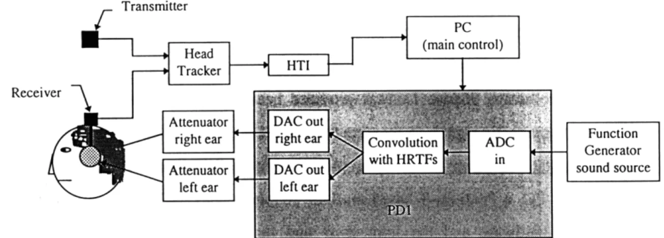
Figure 10 shows a block diagram of the virtual auditory environment used to simulate the acoustic cues.

Transmitter

Receii

Function

- Generator sound source

(27)

3.4. Adaptation Experiment with Feedback

3.4.1. Experiment Description

In each testing run, subjects had to face front (0' azimuth) while a continuous sound (click train) was presented from a random location. When the sound was turned off, they were asked to identify the location of the sound by reporting the position number (i.e., a number between 1 and 13) to the operator, who entered it on the keyboard. As soon as the answer was typed into the computer the appropriate light was turned on as a way of giving a correct-answer feedback. One second after the subject's response, the next random sound was presented. All locations were presented to the subject exactly twice in each run (i.e., the locations were chosen at random without replacement). Thus,

if 13 positions were used, 26 trials were presented in each run. Each run lasts around 3

minutes.

Finally, each run could present either normal or altered cues, determined by selecting the appropriate set of HRTFs.

The basic experimental paradigm was similar to that used by Shinn-Cunningham 1(1994). Each subject performed 8 identical sessions of 40 testing runs each. In each :session, the first 2 runs and the last 8 runs used normal cues, while the others used altered HRTFs. Eight sessions were necessary in order to have a sufficient number of trials to average across. It was assumed that all trials were stochastically independent even though the positions presented were chosen at random without replacement.

Before the beginning of the experiment, subjects were informed that both normal and altered cues would be used at different times and that the apparent location of simulated sources using altered cues may not be their correct location. Also, the subjects were notified every time that a change of cues was about to occur (from normal to altered or from altered to normal), so that they would answer as accurately as possible for the current cues.

(28)

Data from five subjects were gathered. All subjects were naive (without prior experience in auditory localization experiments), reported normal hearing, and had no difficulty performing the test.

3.4.2. Analysis

Bias and resolution were the two quantitative measures used to study the performance and adaptation of each subject under these experimental conditions. Bias measures the error in the subject response (in units of standard deviation), describing how well the subjects adapted to the altered cues. Resolution measures the ability to resolve adjacent stimulus positions.

As described by Shinn-Cunningham (1994), there are three basic processing schemes that can be used for finding estimates of the average signed error (bias) and the response sensitivity (resolution). All schemes assume that each presentation of a physical stimulus results in a random variable with a Gaussian distribution along some internal decision axis. The mean of the Gaussian distribution is assumed to depend monotonically on the source position, while its standard deviation has the same value for all positions. This indicates that the ability to resolve sources comes from the relative distances between their means.

The first estimation method uses a Maximum Likelihood Estimate (MLE) technique to find the means of the internal distributions and the placement of decision criteria, given the confusion matrix observed.

The second method, known as the raw processing method, computes raw estimates of bias and resolution from the means and the standard deviations of the responses. Bias is estimated as the difference between the mean and the correct response divided by the standard deviation. Resolution between two adjacent positions is computed as the difference of the mean responses divided by the average of the standard deviations.

Finally, the third method, also a raw processing method, assumes that the variations in response between the standard deviation of all positions are unimportant. As

(29)

a result, the standard deviation for all positions is averaged and used as a constant value. Bias and resolution are then computed as in the second method.

As Shinn-Cunningham (1994) noted, the results of these three methods are very similar, even though MLE processing is much more computationally intensive and takes into account many factors ignored by the other methods.

Thus, method two was assumed to be adequate for analyzing the data in this study. Accordingly, bias and resolution are given by:

bias m(p)- p (9a)

bias =

m(p + 1) - m(p)

resolution = d'= m (9b)

V (p + 1) J o(p)

where p is the target position, and m(p) and o(p) are the mean and the standard deviation of the responses for target position p, respectively.

3.4.3. Expected Results

Given the results obtained by Shinn-Cunningham (1994) and the linearity3 of the altered cues used in this project, the following results were expected (Figure 11): For the first run using normal cues, subjects are expected to show almost zero bias and better resolution for the center positions than for the edges. When the first altered cues are presented, an increase in resolution in almost all directions was expected (with greater values around zero), due to the fact that the ITDs were larger (doubled) at all positions. Because of the increase in ITDs, the mean response should show a change in slope (with slope of mean response to correct location approximately doubled). This is consistent with subjects hearing sources farther to the side than their correct position. Similarly, we expected that bias would be small for positions near 00 azimuth, larger for intermediate

(30)

positions, and small again at the extreme edges (since subjects could not respond beyond the range of locations presented).

Expected Mean Response

Target Position (degrees)

Expected Bias Characteristic

A • \ i K X_ X a --60 -40 -20 0 20 40 60

Expected Resolution Characteristic

Target Position (degrees) Target Position (degrees)

Figure 11. Cartoon exaggerating the effects of adaptation for mean, bias and resolution.

- : Normal cues. - -: Altered'cues. O: First presentation of normal cues. *: First presentation of altered cues. X: Last presentation of altered cues. +: First presentation of normal cues following the last run of

altered cues.

After the 30th _{altered run, adaptation was assumed to have taken place in that it}

was expected that mean errors would decrease with time. This decrease would be evident by a change in the slope relating mean response to correct location towards one, and a decrease in bias towards 0. Since the acoustic range was larger with the altered cues, the internal decision noise was assumed to grow with adaptation (Durlach and Braida, 1969; Braida and Durlach, 1972; Shinn-Cunningham, 1998). As a result, resolution was expected to decrease with time. The change in internal noise would also cause bias to decrease even farther than if there was no change in stimulus range.

01I'^^^^"^^^'^'

(31)

Finally, results from the first normal cues after exposure to the supernormal cues would give insight into whether subjects really adapted to the supernormal cues or if they were just consciously correcting their responses based on whether they were hearing normal or altered cues. In the first case, subjects could not immediately turn off their remapping of localization cues (even when they were told that they are hearing normal cues) and mean responses were expected to show an after-effect (i.e., the slope relating mean response to location was expected to be less than one). The after-effect should also cause identification performance to be worse after training than before, bias should be non zero and in the opposite direction from the error originally introduced by the remapping. If subjects could consciously change their responses, mean, bias, and resolution should have resembled those from the first normal cue run.

As is shown in Figure 11, the expected results are all symmetrical around 00 azimuth (the mean response had odd symmetry) since there was no reason to think that there would be any left-right asymmetry in the results. For this reason, all the results presented here are collapsed around 00 (i.e., the left and right sides were averaged).

3.4.4. Results

The data showed small differences across sessions, compared to the differences across test runs within a particular session. Therefore, the data reported in this study were collapsed across the eight sessions performed by each subject. The individual subject responses were analyzed to find mean response, bias, and resolution as a function of position for each run in the session. These statistics were then averaged across subjects, and then further collapsed by assuming left-right symmetry, to yield the results shown.

Results from runs 2, 3, 32 and 33 were examined in detail to investigate how performance changed over the course of one session. Run 2 was the last run that used normal cues prior to the exposure to altered cues. At run 2, the subject knew what the experiment was about and should had been comfortable with the procedure. The results of this run served as a baseline or reference point for other runs because it reflected normal

(32)

localization performance. Run 3 was the first run that used supernormal cues and provided a measure of the immediate effects of the transformation. After 30 runs, subjects should have adapted to the unnatural cues, and run 32, the last altered cue used, should illustrate the final state of adaptation. Finally, run 33, the first run using normal cues after the altered cue runs, should revel the after-effect.

Mean response for group with feedback

5( S 4 a) a, c, - 3 c C: 2 o 0 0) a,_o _1' "o V -1

Figure 12. Mean response and slope characteristic for the group with feedback as a function of target position. 0: First presentation of normal cues. *: First presentation of altered cues. --: Normal slope (diagonal). - -: Double slope.

Figure 12 shows the mean response as a function of position. The mean response was very close to the diagonal for the first normal cues presented to the subjects, as expected. When the altered cues were introduced, the outcome was consistent with the transformation employed: subjects heard sources farther to the side and the slope of the response curve was almost doubled for the center positions (the edge effect makes the slope decrease at the borders). Several runs with supernormal cues forced subjects to adapt, decreasing the slope of the mean response and reducing the localization error (Figure 13). However, the localization error was still present because subjects could not adapt completely to the unnatural cues. Finally, when normal cues were presented once

(33)

--again, small localization errors were made (particularly to the sides) in the opposite direction, revealing an after effect from the supernormal cues.

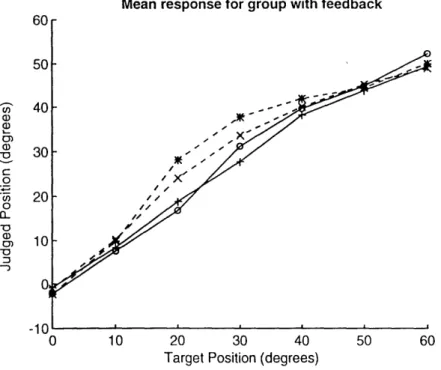
Mean response for group with feedback

tJ E; 4 0), %W C 2 0 -1 '0 0 10 20 30 40 50 60

Figure 13. Mean response for the group with feedback as a function of target position.

-- : Normal cues. - -: Altered cues. 0: First presentation of normal cues. *: First presentation of altered cues. X: Last presentation of altered cues. +: First presentation of normal cues following the last run of altered cues.

As seen in the figures, the mean response at 00 was slightly negative. This negative value was caused by a small (unintended) energy difference between the left and the right ear's HRTFs and it will be discussed in the next section.

Figure 14 illustrates the bias estimates for this group of subjects. As before, the first presentation using normal cues gave reference values. The first altered cue presentation had a large positive bias because subjects heard sources farther to the side than with normal cues. Bias at the edges was negative because the only error that could be made at the extreme locations was towards the center. After adaptation took place, bias was reduced for most locations but it was still greater than the normal bias (adaptation is not complete). Finally, when normal cues were presented again, a negative bias was present for the lateral positions (but not for central positions).

(34)

Bias for group with feedback

0 10 20 30 40 50 60

Figure 14. Bias estimates for the group with feedback as a function of target position.

- : Normal cues. - -: Altered cues. 0: First presentation of normal cues. *: First presentation of altered cues. X: Last presentation of altered cues. +: First presentation of normal cues following the last run of altered cues.

As described before, resolution was expected to increase in almost all the azimuth positions for all runs when using altered cues (it was expected to be somewhat better at the center than at the edges of the range). Figure 15 shows that resolution increased only for the center positions and in the first altered run (where bias had its highest value). Furthermore, the gain in resolution was not as good as the loss of resolution at the side positions. Finally, any changes in resolution between the last altered cues and the first normal presentation after the supernormal runs are small and inconclusive. For both normal and altered cues, there was a substantial decrease in resolution at the end of the session (after training), compared to the beginning of the session (prior to training). This may indicate an overall increase in variability with time, perhaps due to subject boredom. An alternative explanation is that training with the transformation caused decreases in resolution for both normal and altered cues.

In conclusion, the expected results were obtained in this experiment, but the magnitude of the observed changes in performance was small, perhaps because subjects

(35)

adapted very fast to the change in cues. The mean response and the bias showed all the characteristics of adaptation; however, there was only a small after effect, perhaps because subjects learned to go from one cue to the other one consciously. Finally, resolution decreased with training and time.

Resolution for group with feedback

2.5 2 1.5 1 0.5 n 0 10 20 30 40 50 60

Figure 15. Resolution estimates for the group with feedback as a function of target position.

- : Normal cues. - -: Altered cues. 0: First presentation of normal cues. *: First presentation of altered cues. X: Last presentation of altered cues. +: First presentation of normal cues following the last run of altered cues.

3.4.5. Error in Measured HRTFs

The normal HRTFs used had an energy level mismatch at high frequency of 6dB between the left and the right ear at all azimuths in this experiment, causing the subjects to shift their answers towards the left side. While standard deviation should not been affected by the error, the mean response was slightly shifted to the left side. Consequently, bias results also show a small negative shift. Even though mean response and bias were collapsed around 00, this effect was not canceled out completely (especially around 00).

m

(36)

Impulse Response Left Ear (0 degrees)

Impulse Response Right Ear (0 degrees)

400 mV 100 /div 400400 -Start: 0 a 50mV Stop:

Figure 16. Impulse response for the left ear (top panel) and right ear (bottom panel) filters 6dB difference in amplitude is evident for high frequency components.

12.5 dB LogMag 5 dB /div -27.5 180 dog Phase 45 deg /div -180 dog

Frequency Response for Right/Left Ears (0 degrees)

Start: 0 Hz

Start: 0 Hz

Figure 17. Frequency response for the ratio between right and left ear filters difference in magnitude is evident for high frequency components (top panel).

at 0O azimuth. A

at 00 azimuth. A 6dB

Figure 16, the impulse response of the left and right HRTFs at 00 azimuth, shows a difference in amplitude of 50mV or 6dB (i.e., 201loglo[100mV/50mV] ) at the high frequency portions of the signals. This can be verified by examining Figure 17, where the

400 mV 100. mV /div -400 mV

-1

-~1-

__

~AA 31.219 m.. 31.219 ms Stop: 12.8 kHz Stop: 12.8 kHz _____

(37)

frequency response magnitude of the ratio between the right and the left ear is depicted. A 6dB difference is present for the high frequency components (roughly above 7kHz). Both figures represent the actual outputs of the virtual auditory system (i.e., the signals that go directly to the headphones).

3.5. Adaptation Experiment without Feedback

3.5.1. Experiment Description

This experiment was similar in all respects to the previous one, except that no feedback was given to the subjects, and that the trials structure was more tightly controlled. In this experiment each run of 26 trials was broken into subruns of 13 trials each to allow detailed analysis of the speed with which adaptation occurred.

As in the previous test, subjects were informed before the beginning of the experiment that normal and altered cues would be used and that the apparent location of sources using the altered cues might not be the correct location. As before, the subjects were reminded every time before a change of cues would occur (from normal to altered or from altered to normal), so that they would answer as accurately as possible for the current cues.

The purpose of this experiment was to see if removing explicit feedback would slow down the subjects' adaptation process, allowing our measurements to better capture the changes in performance over time. Adaptation was expected to occur even without feedback as subjects adjusted to the larger-than-normal cue range and learned to map the cues to the range of available responses. For example, if they heard a source that appeared outside the possible range of response locations when using altered HRTFs (i.e., between -60' and +600), the subjects would learn to adjust their responses to map the cue range to the response range.

(38)

Data from five subjects were collected, none of whom participated in the first experiments. All subjects were naive, reported normal hearing, and had no difficulty performing the test.

3.5.2. Expected Results

The overall pattern of results expected here was the same as for the previous experiment, except that changes were expected to occur more slowly. Since adaptation took place very fast in the previous experiment, only 10 runs were used here: 2 normal, 7 altered, 1 normal. The shorter session length also prevented subjects from getting bored or distracted towards the end of the experiment.

3.5.3. Results

Runs 2, 3, 9 and 10 were analyzed to investigate how performance changed over the course of one session. As before, run 2 was the last run that used normal cues prior to the exposure to altered cues and provided a baseline against which other runs could be compared. Run 3 provided a measure of the immediate effects of the supernormal cues. Run 9 showed how subjects adapted to the transformed cues after exposure. Finally, run

10 showed any after-effect caused by the exposure to altered cues.

Figure 18 shows the mean response as a function of position. As in the previous experiment, the mean response was very close to the diagonal for the first normal cues presentation. Results after the first presentation of altered cues indicate that subjects heard sources farther to the side with the altered cues, with slope of the response curve roughly doubled for the center positions. After seven runs with supernormal cues, the error in mean response decreased, but subjects never adapted completely (Figure 19). An after-effect showing localization errors in the opposite direction appeared when normal cues were presented in run 10.

Adaption to auditory localized cues from an enlarged head

Adaptation to Auditory Localization Cues

from an Enlarged Head

Salim Kassem

Adaptation to Auditory Localization Cues

from an Enlarged Head

Salim Kassem

ABSTRACT

ACKNOWLEDGMENTS

TABLE OF CONTENTS

1. INTRODUCTION

2. BACKGROUND

2.1. Normal Auditory Localization

2.2.

Auditory Virtual Environments

2.3. Sensory Improvement

source

azimuth

(degrees)

2.41.6

-

0.8Pi 0.0

-

-0.8-

-1.6-

-60 -40 -20

0

20 40 60

Source position (degrees)

4.0

3.0

d'

i

2.0

1.0

0.0

-60 -40 -20

0

20

40

60

Source position (degrees)

3. ADAPTATION TO SUPERNORMAL CUES

3.1. Motivation

3.2. Supernormal Auditory Localization: Double-Size Head

1

(8)

3.3. Equipment and Experimental Setup

3.4. Adaptation Experiment with Feedback

-1

-~1-

__

3.5.

Adaptation Experiment without Feedback