Control of infinite dimensional systems using finite dimensional techniques : a systematic approach

(1)

CONTROL OF INFINITE DIMENSIONAL SYSTEMS USING FINITE DIMENSIONAL TECHNIQUES: A SYSTEMATIC APPROACH

by

Armando Antonio Rodriguez

B.S., Electrical Engineering, Polytechnic Institute of New York (1983)

S.M., Electrical Engineering, Massachusetts Institute of Technology (1987)

E.E., Electrical Engineering, Massachusetts Institute of Techmology (1989)

Submitted to the Department of

ELECTRICAL ENGINEERING AND COMPUTER SCIENCE in partial fulfillment of the requirements for the degree of

DOCTOR OF PHILOSOPHY

at the

MASSACHUSETTS INSTITUTE OF TECHNOLOGY August 1990

@Armando

Antonio Rodriguez, 1990

The author hereby grants permission to M.I.T to reproduce and to distribute copies of this thesis document in whole or in part

Signature of Author:... - ... .

Department of Electrical Engineering anVComputer Science

A

-Certified by: ...

leh sor__ Accepted by: ... ...

Arthur C. Smith, Chairman MASSACHUSETTS INSTITUTE

OF TECHNOLOGY

NOV

27 1990

,ARARIES

ol

. . . .

.-

. . . .

.

. . . . . . . . . . . . . . . . . . . . . . . . . . . . . . . . . . . . . . . . . . . .. . . . . . . . . . . . . . . . . . . . . . . . . . . . . 4.6 Summary .

(6)

5 N** Model Matching Problem 56

5.1 Introduction .. . ... ... .. . .. ... ... .. . . .. .. ... ... . .. . 56

5.2 Infinite Dimensional R** Model Matching Problem . . . 56

5.3 _{Computation of p . . . 71}

5.4 Computation of Hankel Norm . . . 74

5.5 Sequences of Finite Dimensional R** Model Matching Problems . . . 76

5.6 Sum m ary . . . 83

6 Design via R" Sensitivity Optimization 84 6.1 Introduction . . . 84

6.2 R** Approximate/Design Sensitivity Problem . . . 84

6.3 _{Why is the Approximate/Design Problem Hard? . . . 88}

6.4 Solution to ** Approximate/Design Sensitivity Problem . . . 90

6.5 Solution to 7i* Purely Finite Dimensional Sensitivity Problem: Computation of Optimal Performance . . . 98

6.6 Solution to ?** Loop Convergence Sensitivity Problem . . . 100

6.7 Sum m ary . . . 103

7 Design via H** Mixed-Sensitivity Optimization 104 7.1 Introduction . . . 104

7.2 H** Approximate/Design Mixed-Sensitivity Problem . . . 104

7.3 Why is the Approximate/Design Problem Hard ? . . . 108

7.4 Solution to R1** Approximate/Design Mixed-Sensitivity Problem . . . 108

7.5 Solution to IY** Purely Finite Dimensional Mixed-Sensitivity Problem: Computation of Optimal Performace . . . 114

7.6 Poles and Zeros on the Imaginary Axis . . . 114

7.7 Solution to hoo Loop Convergence Mixed-Sensitivity Problem . . . 115

7.8 Unstable Plants . . . 115

7.9 General Weighting Functions . . . 115

7.10 Super-Optimal Performance Criteria . . . 115

7.11 Sum m ary . . . 115

8 Design via 7 2 Optimization 116 8.1 Introduction . . . 116

8.2 R2 _{Approximate/Design Sensitivity Problem . . . 116}

8.3 Why is the Approximate/Design Problem Hard? . . . 119

8.4 Solution to H2 Approximate/Design Sensitivity Problem . . . 120

8.5 Solution to 7 2 Purely Finite Dimensional Sensitivity Problem: Computation of Optimal Performance . . . 125

8.6 Solution to R2 Loop Convergence Sensitivity Problem . . . 126

8.7 Unstable Plants . . . 127

8.8 Mixed-Sensitivity and Super-Optimal Performance Criteria . . . 127

8.9 Sum m ary . . . 127

9 Summary and Directions for Future Research 129 9.1 Sum m ary . . . 129

(7)

List of Figures

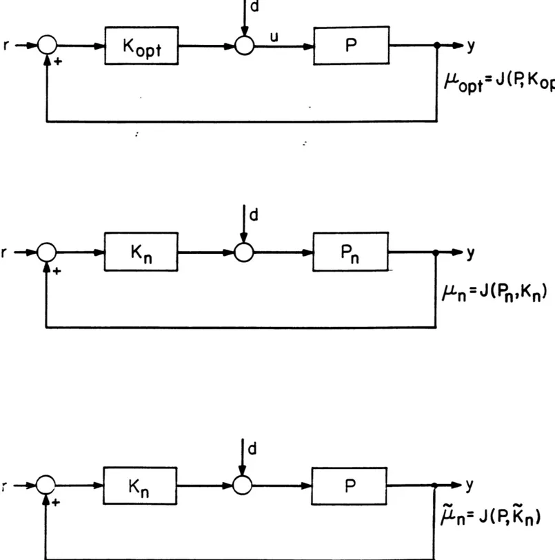
3.1 Feedback Control System Structure. . . . 45 4.1 _{Visualization of Approximate/Design Methodology . . . 53}

(8)

Chapter 1 Introduction & Overview

1.1 Motivation

During the 1980's, the need to address the control of large scale flexible structures has increased immensely. Although this need has arisen primarily from SDI and aerospace applications, it has also been fueled by complexity issues in power distribution and other areas. Because of these driving forces, the problem of designing feedback control systems for infinite dimensional systems has received considerable attention during the past decade. Researchers have endeavoured to develop systematic design procedures. In this thesis such systematic design procedures are presented for a large class of infinite dimensional systems. More specifically, it is shown how to obtain near-optimal finite dimensional compensators for H0 and H2 weighted sensitivity and mixed-sensitivity performance criteria. The approach taken in this thesis is now motivated.

Throughout the thesis, it shall be assumed that the designer has been given a single-input single-output infinite dimensional plant' and a performance measure. In the spirit of the sem-inal work of Zames [59], it will also be assumed that the performance measure has been posed as an infinite dimensional optimization problem. The goal then is to design a near-optimal finite dimensional compensator. The finite dimensionality, of course, is a typical "real-world" implemen-tation constraint. This thesis addresses the problem of designing near-optimal finite dimensional compensators. Two approaches to this problem have appeared in the literature.

The first approach we call the Design/Approzimate approach. In this approach an optimal infi-nite dimensional compensator is designed by solving, if possible, the infiinfi-nite dimensional optimiza-tion problem. The optimal compensator is then approximated by a finite dimensional compensator. This approach will not be considered in the sequel.

The second approach we call the Approximate/Design approach. In this approach the infinite dimensional plant is approximated by a sequence of finite dimensional plants. We then solve a sequence of "natural" finite dimensional problems in which we simply substitute the finite dimen-sional approximants for the infinite dimendimen-sional plant in the original optimization problem. This sequence of finite dimensional problems generate a sequence of finite dimensional compensators which, ideally, will be near-optimal as the plant approximants get "better". Traditionally, however, no such guarantees have been shown.

The key difficulties which have arisen can be attributed to the fact that these performance measures are often not continuous with respect to plant perturbations, even when the uniform topology is imposed. In this thesis, these difficulties are resolved; guarantees are provided.

(9)

The primary motive behind the Approximate/Design approach taken in this work has been that of finding near-optimal finite dimensional compensators for scalar infinite dimensional systems. Other motives can be listed as follows.

(1) Some infinite dimensional models are too complex. It is often very difficult to gain intuition from them. Designing controllers based on such models often requires advanced mathematical machinery and new software. It follows naturally to ask: What would be a "good" finite dimensional approximant? Such an approximant should give immediate insight. To design controllers which are based on such an approximant usually requires little mathematical sophistication. Moreover, much software exists for such a finite dimensional approach. The above question raises the following question: What information about the infinite dimensional plant do we really need in order to achieve the control objective? The approach taken in this thesis attempts to shed light on the above questions.

(2) Some design procedures result in compensators which are infinite dimensional. Such compen-sators may be difficult, if not impossible to implement. The following natural question thus arises: How can we obtain a finite dimensional compensator which is suitable? The Approximate/Design approach taken in this thesis addresses this question directly.

(3) Often, in the early stages of system planning and design, it is necessary to estimate achievable system performance. Such an estimate could be used for system reconfiguration and enhancement. It thus follows that efficient computational tools to obtain such performance information would be extremely valuable to system designers. By taking an Approximate/Design approach, one addresses such computational issues indirectly.

1.2 Related Work & Previous Literature

The problem of designing compensators for infinite dimensional plants has recieved considerable attention during the past decade. Some relevant works are [1], [6]-[10], [13]-[20], [25]-[26], [31]-[38],

[40]-[41], [45], [47], [51]-[53], [57]-[63]. We now give a chronological summary of some of this work. 1950's

The works of [9], [10], and [32] address approximation issues. Real-rational approximation methods are presented. The methods are based on "open loop" ideas and not on closed loop per-formance criteria.

1960's

Much of the technical issues which arise in todays X** model matching approach to control synthesis, were addressed in the famous paper of [51]. In this paper the author solves various interpolation problems in 7Y**. The paper contains the commutant lifting theorem and shows how one can construct norm preserving R" dilations for various operators. This work has been the cornerstone of many approaches/solutions which have appeared for the X** sensitivity and mixed-sensitivity problems.

1970's

The Hankel matrix approximation problem is solved in [1]. This paper has also tremendously influenced the 'H* model matching approach which is present everywhere in the control literature. At the heart of todays model matching approach to control is the ability to parameterize all internally stabilizing compensators for a given plant. Such a parameterization was done in [58] for finite dimensional multivariable linear time invariant plants.

(10)

-An algebra of transfer functions for distributed linear time invariant systems is presented in [4]. Elements in the fraction field of this algebra possess coprime factorizations over the algebra. The work of [58] can thus be used to parameterize the set of all internally stabilizing controllers for plants which lie within the fraction field of the algebra.

1981

In [59], the author posed what is now referred to as the weighted 1X" sensitivity control problem. One objective of this seminal paper was to formulate control problems as optimization problems in an attempt to systematize control system design. It was argued and shown that this frequency

domain approach is natural to handle unstructured uncertainty.

1982

The work of [21] gives a very nice solution for scalar weighted W2 sensitivity and mixed-sensitivity problems.

1983

In [60], the authors use duality and interpolation theory to solve the weighted V"o sensitivity problem for real-rational scalar plants. A fundamental motive for this work was to replace the heuristic aspects of classical design by an explicit mathematical theory.

1984

The commutant lifting theory of [51] is used in [22] to obtain an upperbound for the optimal weighted R" sensitivity associated with scalar finite dimensional systems. The problem of achieving a small sensitivity over a specified frequency band is also addressed. The effects of non-minimum phase zeros is discussed.

A solution to the scalar weighted XV0 mixed-sensitivity problem is presented in [55]. Here the mixed-sensitivity criterion used is that which penalizes the sensitivity and the complementary sen-sitivity transfer functions.

1985

Necessary and sufficient conditions for the existence of finite dimensional compensators for delay systems are presented in [31]. Moreover, it is shown that a stabilizable delay system can always be stabilized using a finite-dimensional compensator.

1986

A method for constructing finite dimensional compensators which stabilize infinite dimensional systems with unbounded input operators is presented in [6]. Applications to retarded and partial differential equations are considered.

In [7], the authors present a method for contructing robustly stabilizing finite dimensional compensators for a class of infinite dimensional plants.

The commutant lifting ideas in [51] are used by [14] to solve the weighted 1" sensitivity prob-lem for the case where the plant is a product of a delay and a real-rational scalar function. Fairly general real-rational weighting functions are considered. The optimal sensitivity and compensator are computed in various situations. The implementation of the optimal infinite dimensional com-pensator is also discussed.

In [18], the authors also solve a weighted R" sensitivity problem using the work of [51]. Here the plant is a delay and the weighting function is first order and strictly proper.

(11)

m

-1987

The ideas presented in [14] are expanded upon in [15].

The results of [18] are extended in [19] to more general delay systems. The plant is assumed to be the product of a delay and a scalar real-rational transfer function with no poles or zeros on the imaginary axis. The weight is assumed to be an RRIX" function which is invertible in X"O . The interaction between delays and non-minimum phase zeros is also discussed.

A solution to the weighted RO" sensitivity problem is presented in [20] for arbitrary scalar distributed plants. An explicit formula is given for the optimal sensitivity. The existence and uniqueness of the optimal compensator is discussed.

In [63], the authors show how the optimal weighted X0 _{sensitivity for a delay can be computed} by solving a two point boundary value problem. Here the weight can be any RX"2' function.

The uniform approximation of a class of delay systems by means of partial fraction expansions is investigated in [62]. Nuclear systems are discussed.

1988

Krein space theory is used to tackle the X" sensitivity problem in [13]. Here the mixed-sensitivity criterion considered penalizes the mixed-sensitivity and complementary mixed-sensitivity functions.

In [16], the authors expand upon the implementation issues presented in [14].

The problem of uniformly approximating delay systems is considered in [45]. Condition for nuclearity are given.

In [25], the authors show how to construct real-rational approximants for nuclear systems. More specifically, it is shown that for this class of systems, balanced or output normal realizations always exist and their truencations converge to the original system in various topologies. Various error bounds are given.

An iterative procedure for constructing near-optimal infinite dimensional compensators for a class of infinite dimensional plants is presented in [57]. The optimality criterion is an R1-* sensitivity criterion. The method presented assumes that the weighting function is strictly proper. In such a case the corresponding Hankel operator is compact.

The computation of the essential spectra of certain Hankel-Toeplitz operator pairs is crucial in the solution of H** sensitivity and mixed-sensitivity problems. This is particularly important when infinite dimensional systems are involved. Such a computation is given in [61]. Calkin algebra techniques are used to obtain the results.

1989

In [8], the author addresses the control of infinite dimensional systems which belong to the algebra presented in [4]. Systems which are of the Pritchard-Salamon class are also addressed.

In [12], the authors present state space formulae to solve a myriad of finite dimensional X2 _and w* control problems.

An FFT-based algorithm for approximating infinite dimensional systems is presented in [28]. When approximating infinite dimensional systems by finite dimensional approximants, the rate at which the approximants converge is very important. Such convergence rate results are given in [26] for certain approximants and infinite dimensional systems. Pade approximations of delays, for example, are discussed.

An H** mixed-sensitivity problem for a flexible Euler-Bernoulli beam is solved in [34]. The solution relies on the techniques used in [41].

In [36], the author uses Laguerre series to approximate certain infinite dimensional systems. Various error bounds are given.

(12)

I

~-'~~--Skew Toeplitz techniques are used in [40], to solve various control problems for infinite dimen-sional systems. The V** mixed-sensitivity problem is addressed.

In [41], the authors reveal the structure of suboptimal X* controllers for distributed plants. In [52], the author shows that fraction field of X** is a Bezout domain. That implies that plants in the fraction field of *' possess coprime factorizations over 7**. This, then allows us to paramerize all stabilizing compensators for such plants using the ideas of [58].

1990

A solution to the ?1 mixed-sensitivity problem is presented in [17]. Here, very general dis-tributed plants and irrational weighting functions are treated.

7** mixed-sensitivity techniques are used in [42] to control unstable infinite dimensional plants. Skew Toeplitz methods are used to derive the controllers.

In [53], the author studies the continuity properties of various XP problems. In particular, it was shown that 1* and N2 _{problems, in general, are discontinuous functions of the plant, even} when the N** topology is used. This paper contains many of the ideas presented in this thesis. It does not, however, address control design. It only addresses certain well-possedness issues which arise in certain optimization problems. We also would like to point out that although elements of this work was initially published in 1987, in a conference proceedings, it did not come to our attention until March 1990.

1.3 Contributions of Thesis

In this thesis, the Approximate/Design Problem is rigorously formulated. A solution is provided for N** and N2 _{weighted sensitivity and mixed-sensitivity performance criteria. These are the main} contributions of the thesis.

More specifically, it is shown that given a "good" finite dimensional approximant for an infinite dimensional plant, one can solve a "natural" finite dimensional problem in order to obtain a near-optimal finite dimensional compensator. Conditions are given which precisely quantify the notion of a "good" finite dimensional approximant.

Given this, the contributions of the thesis can be concretely stated as follows.

(1) A method for constructing near-optimal finite dimensional controllers for a large class of infinite dimensional scalar plants is presented. Stable and unstable plants can be handled. Much software exists to support the necessary computations. The method is thus immediately imple-mentable by practicing engineers.

(2) The same method can be used to construct near-optimal infinite dimensional controllers. One can then "directly" obtain near-optimal finite dimensional compensators by approximating the infinite dimensional controllers. This approach, however, goes against the spirit of the thesis since it requires that we solve an infinite dimensional optimization problem.

(3) The most commonly used design criteria have been addressed; i.e. N"* and N2 _weighted sensitivity and mixed-sensitivity problems. Again, much software exists to support our finite di-mensional approach to these paradigms.

(4) For a large class of N"* weighted sensitivity/mixed-sensitivity problems, the optimal perfor-mance can be easily computed by solving a sequence of finite dimensional eigenvalue/eigenvector

(13)

problems rather than the typical infinite dimensional eigenvalue/eigenfunction problems which appear in the literature. The methods presented apply even in situations where the associated Hankel/Toeplitz operators are non-compact.

Such information can be used to determine fundamental performance limitations for a given system; e.g. best possible £2 disturbance rejection, robustness, etc. It can thus be used to guide

designers (engineers, pilots, etc.) during the initial stages of system development, design, and configuration.

Analogous results are presented for the X2 design criteria considered.

(5) The thesis sheds light on such issues as what a "good" finite dimensional approximant is and hence on what information is needed in order to achieve a particular control objective. It is shown that appproximations should be based on the control objective; not on open loop intuition. Moreover, it is shown that open loop intuition can often be quite misleading. These ideas have potential implications in such fields as system identification and decentralized control.

1.4 Organization of Thesis

The remainder of this thesis is organized as follows.

In Chapter 2, notation and results from complex variable and approximation theory are pre-sented. The function spaces H** and R 2 are defined and discussed. Various notions of convergence are presented.

In Chapter 3, results from algebraic system theory are presented; e.g. the Youla parameteriza-tion and the Corona theorem.

In Chapter 4 three problems are formulated. They are the A-Norm Approximate/Design J-Problem, the K-Norm Purely Finite Dimensional J-J-Problem, and the K-Norm Loop Convergence J-Problem. In the sequel, the

K

will represent HX** and X2 norms. The J will represent sensitivity and mixed-sensitivity performance criteria.

The K-Norm Approximate/Design J-Problem addresses the problem of finding near-optimal finite dimensional compensators. The K-Norm Purely Finite dimensional J-Problem addresses the issue of computing the optimal performance using finite dimensional techniques. The

K-Norm

Loop Convergence J-Problem addresses the question of what additional properties are exhibited by designs based on the Approximate/Design approach advocated in the thesis. The above three problems are considered in the sequel for Ro* and R 2 weighted sensitivity and mixed-sensitivity performance criteria.

In Chapter 5, the H** Model Matching Problem is defined and discussed. It is shown how near-optimal solutions can be constructed. The results presented here are exploited heavily in subsequent chapters on R0* design.

In Chapter 6, the focus is on designing near-optimal finite dimensional compensators based on *

00 _{sensitivity design criteria. More specifically, in this chapter a solution is presented to the R**} Approximate/Design Sensitivity Problem, the H0 Purely Finite Dimensional Sensitivity Problem, and the 7** Loop Convergence Sensitivity Problem. For simplicity, stable and unstable plants are treated separately.

In Chapter 7, the focus is on designing near-optimal finite dimensional compensators based on R0 mixed-sensitivity design criteria. More specifically, in this chapter a solution is presented to the N** Approximate/Design Mixed-Sensitivity Problem, the R0 Purely Finite Dimensional Mixed-Sensitivity Problem, and the N00 Loop Convergence Mixed-Sensitivity Problem.

(14)

on R2 sensitivity/mixed-sensitivity design criteria. More specifically, in this chapter a solution is

presented to the H2 Approximate/Design Sensitivity Problem, the H2 _{Purely Finite Dimensional}

Sensitivity Problem, and the H2 Loop Convergence Sensitivity Problem. The analogous

mixed-sensitivity problems are also addressed. The features which distinguish the X2 case from the R** case are highlighted.

Finally, Chapter 9 summarizes the results of the thesis and suggests possible directions for future research.

(15)

-Chapter 2

Mathematical Preliminaries:

Notation & Function Theory

2.1 Introduction

In this chapter we establish notation to be used throughout the thesis. Some essential mathematical results are also presented. More specifically, the normed linear spaces H2 and Roo are defined and discussed. Various notions of convergence in HX1" are presented; e.g. uniform and compact convergence. Results from hX-"* approximation theory are also presented. Examples are given to illustrate some of the ideas. Most of the material presented in this chapter can be found in [2], [5],

[30], [33], [35],

[44],

[49], [56]

1.

2.2 Some Notation & Definitions

Throughout the thesis, we will use the symbols C, R, and Z to denote the complex, real, and integer numbers, respectively. C, and Re will be used to denote the extended complex and real numbers. The open right and left half complex planes will be denoted C+ and C_. R+ and Z+ will be used to denote the non-negative real numbers and positive integers.

I()|

and (.) will denote the magnitude (modulus) and complex conjugate of the complex quantity (-). () and L(.) will be used to denote the phase angle of the complex quantity (.). The symbol

j

will be used to denote the purely imaginary number VT.

The greek letter e shall always be used in proofs to denote a given strictly positive, but arbitrarily small, quantity. With this convention we can avoid the excess verbage "given e > 0, however small,...".

Given sets A and B, A C B and A C B will be used to denote strict and non-strict containment of A within B. The symbol A/B will denote the set of points in A which are not in B. A U B and

A

n

B will denote the union and intersection of the sets, respectively.

In the mathematics literature the characteristic function of a set S is defined as that function

which is unity on S and zero elsewhere. It is typically denoted XS. Throughout the thesis we shall predominantly work on the imaginary axis. This motivates the following definition which we introduce strictly for notational economy.

'Extra material has been included in this chapter in order to make the thesis self-contained and to facilitate future addenduns.

(16)

Definition 2.2.1 (Characteristic Function)

Let S denote a subset of the extended real numbers. In what follows, the map Xs : jS -+ {0, 1} will denote the characteristic function of the set

jS;

i.e.

Xs(jw)

cf

1 w

E S;

0 elsewhere.

Convention 2.2.1 (Transform Pairs)

We shall often use f(t) or

f

and F(s) or F, to denote Laplace, Fourier, Plancherel transform pairs. Here

f

(lowercase) will denote a time function and F (uppercase) will denote its transform. The interpretation should be clear from the context.

Convention 2.2.2 (Lebesgue Integral)

All integrals in this thesis shall be assumed to be Lebesgue integrals [49], unless otherwise stated. Any measure-theoretic statements which appear are made with respect to Lebesgue's measure unless otherwise stated 2.

Let f(t) denote a real-valued Lebesgue measurable function defined on a set S C R. Definition 2.2.2 (Support of a Function)

The support of

f,

denoted suppf, is defined to be the closure of the set where

f

takes on non-zero values; i.e.

def

suppf = closure{t E S

I

f(t)

$

0}.

I

Definition 2.2.3 (Essential Supremum of a Function) The essential supremum of

f

on S is defined as follows

ess sup

f

e inf{ M E Re

I

measure( {t E S I f(t) > M} ) = 0

}.

M

Here measure(.) denotes the Lebesgue measure of the set

(-).

U

Definition 2.2.4 (Convolution of Functions)

Given any two time functions

f

and g with support on R, their convolution will be denoted

f

* g and defined as follows

(f

* g)(t) jef

L

f(t -

r)g(r )dr.

2

(17)

I

Throughout the thesis we will deal with normed linear spaces.

IIf II(.)

will be used to denote the norm of a function f belonging to the normed linear space (.).

Definition 2.2.5 (Isometry, Isomorphism)

Let

N1

and A2 be normed linear spaces. A norm preserving linear operator from Ar1 to A2 is called

an isometry. Such operators are necessarily injective (one-to-one). They need not be surjective (onto). Ar1 and A2 are said to be isomorphic if there exists a bijective bounded linear operator from Arl to A2 whose inverse is also bounded (cf. definition 2.8.1). The operator is called an

isomorphism. A surjective isometry is an isomorphism. We call such an operator an isometric isomorphism.

In what follows we shall deal with the normed linear spaces 2 and N*. They shall be defined shortly.

2.3 Single-Valued Complex Functions

In this section we present standard definitions and results from the theory of complex functions of a single complex variable. Let F(s) or F, denote a complex-valued function of a single complex variable s. We assume all such functions to be single-valued unless otherwise stated. Let so denote any point in the finite complex plane.

Definition 2.3.1 (Domain and Boundary)

A domain is a non-empty open connected subset of the extended complex plane. The boundary of a domain V shall be denoted OD.

The open right half plane is a domain. Definition 2.3.2 (Domain of Definition)

The domain of definition of a single-valued complex function is a domain in the complex plane over which the function is defined.

In the sequel, the domain of definition of a function will be ascertainable from the context. It will usually be the region of convergence of the function when viewed as the Laplace Transform of a time function.

Definition 2.3.3 (Analytic and Entire Functions)

We say that F is analytic at the point so, if F is differentiable at all points in some open neighbor-hood of so. We say that F is analytic within a domain D, if it is analytic at each point within D. If F is analytic within C, then we say that F is an entire function.

(18)

- I1

Proposition 2.3.1 (Taylor Series)

Let F be analytic at the point

a

= so. Given this, there exists a neighborhood

N(so, R)

{s

E C

I

Is -

sol

< R}

about so, and a sequence {am}'o, such that 00

F(s) = E am(s - so)"

m=O

for all s E N(so, R). Moreover,

am = F(m)(so)

and the series converges uniformly on all compact subsets within the neighborhood. We shall refer to this representation for F as the Taylor series expansion for F about so.

U

The radius of convergence, of the Taylor series for F about so is equal to the distance from so to the nearest singularity of F (cf. definition 2.3.7). It is given by Hadamard's formula

Ro =I

limn+oo sup V/a 7 Definition 2.3.4 (Zero of a Function)

We say that so is a zero of F, if

lim F(s) = 0

8--+80

along any path in the domain of definition of the function F.

Definition 2.3.5 (Multiplicity of a Zero for Analytic Functions)

Let F be analytic at s = so. Also, let so be a zero of F. We say that so has multiplicity m E Z+, if there exists a function G such that for all s in a neighborhood of so,

F(s) = (s - so)mG(s) where G(so) j 0 and G is analytic within the neighborhood.

I

An integer m and a function G can always be found for any single-valued function F. In this sense, all single-valued functions exhibit polynomial behavior near a zero. It must be noted that for single-valued functions obtained from multi-valued functions, the situation is different. Such functions shall be discussed in the next section.

Definition 2.3.6 (Roll-off)

(19)

Definition 2.3.7 (Singularity, Isolated Singularity)

If F is not analytic at so, then we say that s = so is a singularity of F. If there exists a neighborhood

around so which contains no other singularities of F, then we say that so is an isolated singularity of F.

It is standard convention by authors to assume that oo is a singularity. This convention shall receive further consideration below. A zero at oo, we shall see, should be viewed as a removable singularity (cf. definition 2.3.8).

Proposition 2.3.2 (Laurent Series)

Let so be an isolated singularity of F. Given this, there exists an annulus

A(so, ri, r2) {s E C

I

r1 < |s - so

l

< r2)

about so, and sequences {am}m*o, {bn}* 1 , such that

00 00

F(s) = am(s

-

so)m

+ E

bn 1

m=O n=1

for all

s

E A(so, ri, r₂_{). Moreover, the convergence is uniform on all compact subsets of the annulus.}

We shall refer to this representation for F as the Laurent expansion for F about so. The second summation, which consists only of negative powers of (s - so), is called the principal or singular

part of F at so.

Let so be an isolated singularity of F. Definition 2.3.8 (Removable Singularity)

The point s = so is said to be a removable singularity of F, if lim (s - so)F(s) = 0

8-+30

along any path in the domain of definition of F [2, pp. 124].

One can show that the above is equivalent to F having no principal part. In such a case, the function can be made analytic at so, simply by redefining it at the point.

One can also show that so is removable if and only if

IF(s)I

is bounded in some annulus about SO. This condition is due to Riemann.

Definition 2.3.9 (Pole)

If lim,_.,, F(s) = oo, along any path in the domain of definition of F, then we say that the point s = so is a pole of F.

One can show that this is equivalent to F having a principal part with only a finite number of terms.

(20)

Definition 2.3.10 (Multiplicity of a Pole)

Let so be a pole of F. We say that it is a pole with multipliciity m, if so is a zero of " with multiplicity m.

Definition 2.3.11 (Improper Function) We say that F is improper if oo is a pole of F.

Definition 2.3.12 (Rational Function)

We say F is a rational function, if it is the ratio of two polynomials; each of finite degree. We say that it is real-rational, if the coefficients of the numerator and denominator polynomials are real.

U

Rational functions have a finite number of poles and zeros. They also possess singularities at o which are removable.

Definition 2.3.13 (Meromorphic Function)

F is said to be meromorphic in a domain D if the only singularities within V are isolated poles. If V = C, then we just say that the function F is meromorphic.

The functions F(s) = and G(s) =

2-.

are examples of a meromorphic functions.

A meromorphic function can only have a finite number of poles in any compact set. If a meromorphic function has an infinite number of poles, then they must cluster at oo.

It can be shown that a meromorphic function F with a finite number of poles is necessarily the ratio of an entire function over a polynomial.

It can also be shown that meromorphic functions are necessarily the ratio of two entire functions. Definition 2.3.14 (Essential Singularity)

We say that so is an essential singularity of F, if the principal part of its Laurent expansion about so has an infinite number of nonzero terms.

One can show that this can occur if and only if so is a singularity of F which is neither removable nor a pole.

Singularities at oo are treated as follows. Definition 2.3.15 (Singularities at oo)

s = co is a removable singularity, a pole, or an essential singularity of F(s), if ( = 0 is a removable singularity, a pole , or an essential singularity of FQ).

I

The functions e-8 and e have essential singularities at oo and 0, respectively.

(21)

Proposition 2.3.3 (Picard's Theorem)

A complex-valued function F in any neighborhood of an essential singularity assumes all values except possibly one.

This proposition is often referred to as Picard's Theorem. A weaker version of the theorem, known as the Casorati-Weierstrass Theorem, appears in [33, pp. 158].

The above shows that isolated singularities of otherwise single-valued analytic functions must either be removable singularities, poles, or essential essential singularities.

The following proposition characterizes "maxima" of analytic functions on a domain [2, pp. 134], [33, pp. 150], [49, pp. 212, 249, 253-259]. It is known as the Mazimum Modulus Theorem. Proposition 2.3.4 (Maximum Modulus Theorem)

Let F be analytic within a domain D. Then

IF(s)|

achieves its maximum within D if and only if F is constant. If the domain D is bounded, then we have

IF(s)|

5 sup

IF(s)|

8EOD for all s E D.

The above does not imply that an analytic function F on a domain will achieve its maximum on the boundary. The following example illustrates this point.

Example 2.3.1 (Unbounded Analytic Function on a Strip)

The function F(s) = ee' is an entire function. Consider it over the unbounded domain jIm(s)| I . It does not achieve its maximum modulus on the boundary. Its magnitude on the boundary is 1. Within the domain, however, the function grows exponentially along the positive real axis.

The following proposition can be found in [2, pp. 127], [49, pp. 209]. Proposition 2.3.5 (Uniqueness of Analytic Functions)

Let F and G be analytic within some domain D in the complex plane. Let S be a subset of D. If

S has an accumulation point in V and F = G on S then F = G throughout D.

I

This proposition implies that the zeros of a non-constant analytic function cannot accumulate within its domain of analyticity. If they do, then the function must be identically zero over the entire domain. This property is due to the fact that the zeros of a single-valued analytic function are necessarily isolated within its domain of analyticity.

2.4 Multi-Valued Complex Functions

In this section we consider multi-valued complex functions of a single complex variable. Such functions, as we shall see, can be viewed as a collection of single-valued functions. Let F denote a

complex valued function of a single complex variable s.

In order to precisely define multi-valued functions, we define the concept of a branch point as follows. A branch point is a singularity that is associated with multi-valued functions only.

(22)

Definition 2.4.1 (Branch Point)

The point a = so is a branch point of the function F, if when we travel around the point, along a sufficiently small circle, we do not return to the same value; i.e. for r > 0, sufficiently small,

F(so + r) / F(so + re'2-).

Branch points at oo can be defined similarly by considering balls around the point at oo. Such a ball could be precisely defined in terms of the Riemann sphere associated with the complex plane. An equivalent approach is provided by the following definition. The definition parallels that given for singularities of single-valued functions at oo in definition 2.3.15.

Definition 2.4.2 (Branch Points at oo)

The point s = oo is a branch point of the function F(s), if ( = 0 is a branch point of F().

I

Definition 2.4.3 (Multi-Valued Function)

F is a multi-valued function if it posseses a branch point in its domain of definition.

The function F(s) = v/s -1, for example, is multi-valued. It posseses a branch point at s = 1. The analytic study of multi-valued functions usually requires that the multi-valued function be expressed in terms of single-valued functions. One way of doing this is to consider the multi-valued function in a restricted region of the extended complex plane. Then, one chooses a value at each point in such a way that the resulting single-valued function is continuous on the restricted domain.

This motivates the following definition.

Definition 2.4.4 (Branch of a Multi-Valued Function)

A continuous single-valued function obtained from a multi-valued function is called a branch of the multi-valued function.

Definition 2.4.5 (Branch Cut)

Typically, to obtain a branch, one must delete some curve in the s-plane. Such a curve is typically referred to as a branch cut. The curve is such that if not crossed over, the function remains single-valued. Given this, we have that a branch cut is a line or curve of singular points introduced in defining a branch of a multi-valued function.

U

The branch cuts of a multi-valued function are not unique. A given branch cut, however, uniquely defines a distinct branch of the multi-valued function. Branch points are conunon to all branch cuts of a multi-valued function. A branch is also uniquely determined once a particular value of the multi-valued function over the restricted domain has been specified. Specifying such a value automatically determines the branch cut. This follows by continuity.

(23)

Definition 2.4.6 (Complex Logarithm)

Let ln(.) denote the real-valued natural logarithm from elementary calculus. The complex logarith-mic function is denoted Inm(.) and defined by the equation

def

nm =(s) IlnIs + jO(s)

where s =

Islei(3)

is any extended complex number and Inm,(O) =f -oo and In,,(oo) ' 00.

I

To see that this function is multi-valued we consider a circle of radius one centered at the origin of the complex plane. We then note that if the circle is traversed in the conterclockwise direction, then Inm,(.) does not return to its initial value. We have, for example, Inm,(le3) = 0 + jO and Inmv(le12_{w) = 0 + j2r. The origin is thus a branch point of the complex logarithmic function.} Given this, we see that it is a multi-valued function. One can show that the point s = oo is also a branch point. To obtain a branch of this function we proceed as follows.

Let

def

S = Ce/{-oo < Re(s) < 0; Im(s) = 0} = {s E C

I

- r < 6(s) <7r

}

denote the set of points in the extended complex plane obtained by deleting the extended negative real-axis. S defines a branch cut for the complex logarithmic function.

Definition 2.4.7 (Principal Angle)

We define the principal angle function O,, : S/0 -+ (-r, r) as follows tan-1 W 0

> 0;

6,,s) ' -tan-' + o < 0; o > 0; - tan" - 7r a < 0; W < 0

where s = a +

jw.

We note that ,, is continuous on S/0. Definition 2.4.8 (Principal Logarithm)

Given the above, the principal branch of the complex logarithmic function is defined on S as follows def

ln,,(s) = InIsI+ j0p(s)

for s

$

0, In,(0) 00 , and In,(oo) de 00.

This function is analytic, as well as continuous, on S. The negative real-axis is the associated branch cut. Other branch cuts and branches of the logarithmic function can similarly be defined.

Now we consider another multi-valued function. It is defined as follows. Definition 2.4.9 (Complex Power Function)

Let c be a fixed real number. Given this, we have

(8C)Mv t ecln-,(s)

(24)

I

The principal branch of this function is defined by using the principal logarithm In,,(.) as follows.

Definition 2.4.10 (Principal Power Function)

(S Z)P 4f ez np (s)

Proposition 2.4.1 (Analytic Branches)

Given a multi-valued function, an analytic branch F can always be constructed in any domain which does not contain a branch point.

U

This convention shall be adopted throughout the thesis for all multi-valued functions considered. Given this, functions such as

F~s = 1 2 3 -lisj 4

F) s + 1 s+ 2 s+3 s+4

will be regarded as analytic in the extended open right half plane and continuous everywhere on the extended imaginary axis.

It was seen in the previous section that single-valued functions exhibit polynomial behavior near zeros. This is not the case for single-valued functions which are constructed from multi-valued functions. The function F(s) = fs, for example, exhibits irrational behavior near s = 0. We thus have the following definition.

Definition 2.4.11 (Algebraic Multiplicity of a Zero)

Let F be a branch of a multi-valued function. Let F be analytic at s = so. Also, let so be a zero of F. We say that so has algebraic multiplicity m E R+, if there exists a function G such that for all s in a neighborhood of so,

F(s) = (s - so)m G(s)

where G(so)

$

0 and G is analytic within the neighborhood. Here the neighborhood is assumed to lie within the domain of definition of the branch F.

A non-negative real nmnber m and a function G can always be found for any analytic branch F of a multi-valued function.

2.5

£2

Function Theory

The function space L2 is defined as follows.

(25)

Definition 2.5.1 (Function Space: C2 (R))

,2 4f 12(R) will denote the space of Lebesgue square integrable complex-valued functions with support on R. C2(R+) and £2(R-) are similarly defined. C2 is a normed linear space over the field

C, when endowed with the following norm

||f||,C2

|f(t)|2dt.

The £2 functions should be thought of as the set of all finite energy time signals.

The space £2 is also an inner product space when endowed with the following inner product

< f, g >,C2 f0f(~tig(t)dt.

Moreover, it is complete with respect to this inner product. £2 is thus a Hilbert space.

The following proposition can be found in [35]. It is the basis for classical projection theory. Proposition 2.5.1 (Classical Projection Theorem)

Let H denote a Hilbert space withe inner product

<

-,. >,H. Let M denote a closed subspace of X. Given x E ?Y there exists a unique element mo C M such that

min

JJ

- m||. = ||z - mJ||H.

mEM

Moreover, x - m, E M' where

M' {x E i < x, -t m >%= 0 m E M}. We say that m, is the projection of x onto M and write

Mo = fMX. Also, R is the direct sum of calM and calM'; i.e.

This notation means that each element x c H can be written as X = m1

+

m2 where mi E M and

m2

E

M'.

From the classical projection theorem, it thus follows that f 2

(R) is the direct sum of £2(R+) and C2(R_):

=2(R) = E2(R+) @ £2(R);

i.e. given

f

c E2(R) there exists unique functions

f+

E E2(R+) and

f-

E 2(R_), such that

f

=

f+

+

f_.

This is because C2(R_) is the orthogonal complement of E2_{(R+) in £}2_(R).

Definition 2.5.2 (Function Space: L2_(jR))

One can also define the space L2_{(jR) as the set of all complex-valued functions which are Fourier/Plancherel}

transforms of £2(R) time functions. £2(jR) is a normed linear space over the field C when endowed

with the following norm

|FeC2

_ii~iic( 1

|

iF(jw) 2

dw.

(26)

U

Parseval's theorem tells us that C2 (R) and E2(jR) are isomorphic. More specifically, it shows that

li| IC2(R)

=

||F11c2(jR).

Since C2(R) and C2_{(jR) are isometrically isomorphic, there is no need to distinguish between}

the spaces. We shall usually just write C2. _{Which space is being considered should be apparent}

from the context.

The function space ?j2 is defined as follows. Definition 2.5.3 (Function Space: 7J2)

72 4- 2_{(C+) will denote the Hardy space of complex-valued functions which are analytic in C+} and uniformly Lebesgue square integrable on lines parallel to the imaginary axis in C+. ?y2 is also a normed linear space over the field C, when endowed with the following norm

||Fllu

2

=L

sue -

|F(o-

+

js)|

2

dw.

?X2 _{consists exactly of those functions which are Laplace/Plancherel transforms of}

£2(R+) functions [29, pp. 100, Paley-Wiener Theorem]. Consequently, there is no need to distinguish between R2 and

£

2(R+). They are isomorphic.

Definition 2.5.4 (Function Space: h2±)

Analogously, H2J _{will be used to denote the space of functions which are Laplace transforms of} functions in C2

(R_).

It is a fact [30, pp. 128] that ?X2 and 2L _{functions can be unitarily extended to have support} almost everywhere on the imaginary axis. More precisely, we have the following proposition. Proposition 2.5.2 (Extension of ?J2 Functions onto the Imaginary Axis)

Given F E ?j2, _{it possesses non-tangential limits almost everywhere on the imaginary axis. By} taking such limits, one obtains a unique extension

P

E £2 of F onto the imaginary axis. Moreover, this extension is an isometry.

I

A similar proposition applies for functions in H2-. When dealing with R2 and R2 J functions we shall always assume that we are dealing with the extended functions; i.e. we make no distinction between the function and its extension. Given this, the norms of such functions can be computed from values on the imaginary axis. This gives us the following proposition.

Proposition 2.5.3 (Norm of 12 Functions) Given F E 1i2, we have

(27)

I

The following notation shall be used to denote the various projection operators on C2_.

Definition 2.5.5 (Projection Operators on £2)

The projection of C2 onto L2(R+) ( or R2) shall be denoted llc2(R+) ( or Hu2) . These operators shall be used interchangeably. The projection of C2 onto £2_{(R_) (or X2') shall be denoted}

HC2(R-)

(or R.U). 2 These operators shall be used interchangeably.

We note that such projection operators have induced norms, on £2, equal to 1.

2.6 LO Function Theory

The function space E** is defined as follows. Definition 2.6.1 (Function Space: C**(jR))

,o w 4f**(jR) will denote the space of Lebesgue measurable essentially bounded complex-valued

functions with support on the imaginary axis. This space is a normed linear space over the field

C, when endowed with the following norm

||F||.

=

ess sup |F(jw)I.

wE Ri

Proposition 2.6.1 (System Interpretation)

Given F E VC*, the associated time function

f

defines a convolution kernel from £2 to £2. Moreover,

|IF||LM

= sup

|if

* X||C2

where

f

* x denotes the convolution of

f

with x.

U

Definition 2.6.2 (Adjoint)

Given a complex-valued function F(s) with domain of definition including the imaginary axis, we shall denote the adjoint of F as follows

F*(s) d F(-)

Strictly speaking, the concept of an adjoint should be defined in terms of bounded linear functionals [48]. This degree of rigor will not be necessary for our purposes.

The function space C,(jR) is defined as follows. Definition 2.6.3 (Function Space: Ce(jR) )

Ce df C,(jR) is the set of all complex-valued functions which are continuous on the extended imaginary axis.

(28)

2.7 'W Function Theory**

The function space W"' is defined as follows. Definition 2.7.1 (Function Spaces: X", RO")

def

H 0=

7-

(C+) will denote the Hardy space of complex-valued functions which are analytic and essentially bounded in C+.

1"-

is a normed linear space over the field C, when endowed with the norm

|IFII% I sup sup jF(u +

jw)I.

a>O WERe

RO 7"(C+) will denote the subspace of R" functions which roll-off.

RIX" and R1"1 will denote the corresponding subspaces of real-rational X" functions. We note that Ri"" functions have no poles in the extended closed right half plane [23]; i.e. all of their poles lie in the open left half plane.

Definition 2.7.2 (Function Space: X(C_))

1"(C_) will denote the Hardy space of complex functions which are analytic and essentially bounded in C.

I

RX" (C_) will denote the corresponding subspace of real-rational functions. Such functions have no poles in the extended closed left half plane [23]; i.e. all of their poles lie in the open right half plane.

Definition 2.7.3 ( 1B)

1B 4'f XB(C+) will be used to denote the Hardy space of complex-valued functions which are

analytic in C+ and bounded on compact subsets within C+ [60, pp. 589].

This space should be thought of as containing all improper functions which would be in 1" if it were not for their improperness (e.g. f(s) = s). RRB will denote the corresponding subspace of real-rational functions.

It is a fact [30, pp. 128] that 1"' functions can be unitarily extended to have support almost everywhere on the imaginary axis. More precisely, we have the following proposition.

Proposition 2.7.1 (Extension of R" Functions onto the Imaginary Axis)

Given F

E

-", it possesses non-tangential limits ahnost everywhere on the imaginary axis. By taking such limits, one obtains a unique extension F E L"" of F onto the imaginary axis. Moreover, this extension is an isometry.

I

When dealing with such functions we shall always assume that we are dealing with the extended functions; i.e. we make no distinction between the function and its extension. Given this, the norms of such functions can be computed from values on the imaginary axis. We state this formally as follows.

Control of infinite dimensional systems using finite dimensional techniques : a systematic approach

@Armando

NOV

27

1990

ARCHIVES

Contents

ol

. . . .

. . . .

.-

. . . .

.

List of Figures

Chapter 1

Introduction & Overview

1.1

Motivation

1.2

Related Work & Previous Literature

1.3

Contributions of Thesis

1.4

Organization of Thesis

K

K-Norm

-Chapter 2

Mathematical Preliminaries:

Notation & Function Theory

2.1

Introduction

[30], [33], [35],

[44],

[49], [56]

1.

2.2

Some Notation & Definitions

I()|

j

n

jS;

Xs(jw)

1

w

E S;

0 elsewhere.

f

f

f,

f

I

$

I

f

f

I

}.

(-).

U

f

f

(f

L

r)g(r )dr.

I

IIf II(.)

N1

2.3

Single-Valued Complex Functions

a

N(so, R)

{s

E C

I

Is -

sol

< R}

U

8--+80

I