Continued development of the QUANDRY code

CONTINUED DEVELOPMENT OF THE QUANDRY CODE by

A.F. Henry, Philippe Finck, Han-Sem Joo, Hussein Khalil, Kent Parsons, Jos6 Perez Energy Laboratory Report No. MIT-EL 84-001

A.F. Henry Philippe Finck Han-Sem Joo Hussein Khalil Kent Parsons Jose Perez Energy Laboratory and

Department of Nuclear Engineering Massachusetts Institute of Technology

Cambridge, Massachusetts 02139

Sponsored by

Consolidated Edison Company of New York Northeast Utilities Service Company

Pacific Gas & Electric Company PSE&G Research Corporation

under the

MIT Energy Laboratory Electric Utility Program

MIT Energy Laboratory Report No, MIT-EL 84-001

Final Report on Continued Development of the QUANDRY Code

I. Introduction

This report is a summary of the continued development and testing of the nodal code QUANDRY as applied to the analysis of detailed power distributions throughout the lifetime of light water moderated power

reactors. The project has been supported by four utilities, Consolidated Edison Co., Northeast Utilities Services Co., Pacific Gas and Electric Co., and Public Service Electric and Gas Research Corp. The duration of the project was originally to be from September 1982 to September 1983. However, in order to provide continued support for students during the 1983 Fall term and to get into phase with utility budgeting schedules, charges for faculty supervision were reduced and a no-cost extension for the period October 1983 through December 1983 was requested and agreed to.

The general goal of the work carried out has been to develop and test a method for predicting detailed power history throughout the lifetime

of a light water moderated power reactor. We have based the scheme on the two-group nodal code QUANDRY, and the present work has been con-cerned with testing and refining that code so that it can be used to predict

accurate values for local fuel-pin power throughout reactor lifetime in a straightforward, economical manner. The study has been concerned with three tasks:

1. Testing in three dimensions.

2. Reconstruction of detailed flux shapes for three-dimensional nodes.

3. The determination of albedoe boundary conditions.

The completion of these tasks has led us to the conclusion that a production code embodying the QUANDRY scheme would be more

accurate, more reliable, easier to run, and ultimately cheaper than the present nodal methods used by utilities.

II. Review of the Theory

Before presenting any results it will be helpful to review the theory, that underlies QUANDRY.

The basic unknowns in QUANDRY are the two-group volume-averaged nodal fluxes. Node-face-averaged currents and fluxes also appear in the basic equations. For the ideal case of reactors composed of nuclearly homogeneous nodes, QUANDRY predicts the node-averaged fluxes very accurately (maximum error ~ 2% for nodes 20 cm on a side). However, real LWR's are not nuclearly homogeneous, and the problem of finding "homogenized" cross sections that will reproduce the correct

node-integrated reactor rates is a severe one. In fact, it can be shown that, if the conventional diffusion theory group-parameters and continuity

conditions are employed, there is no set of homogenized cross sections that will reproduce reference results. QUANDRY circumvents this difficulty by permitting the face-averaged fluxes to be discontinuous across nodal interfaces. To accomplish this we have introduced

"discontinuity factors" into QUANDRY. If correct values of these factors are provided, QUANDRY will reproduce exactly the nodal reaction rates of the standard model. The discontinuity factors are defined as the ratio of the true face-averaged group-flux for the node in the heterogeneous reactor to its value predicted by the basic nodal equations (the so-called "nodal coupling equations") when node-averaged group parameters and

I ik

-3-used in those equations. It follows that, if correct discontinuity factors are used, the node-averaged fluxes, reaction rates, and the eigenvalue predicted by QUANDRY will be exact. Moreover, it is then possible to regenerate exactly face-averaged fluxes for the heterogeneous nodes making up the reactor. These latter quantities can be used to obtain approximate values of node corner-point fluxes by an interpolation method. Knowledge of face-averaged and corner-point fluxes then

permits reconstruction of detailed flux shapes throughout a heterogeneous node.

Determination of "exact" discontinuity factors requires knowing the "exact" solution. _{Thus, in practice we must approximate. A basic} ground rule which we have imposed on our approximate procedures for finding discontinuity factors and homogenized group parameters is to avoid quarter-core solutions and to obtain fine-mesh solutions with reactor

heterogeneities represented explicitly only for regions the size of a single assembly, or, at most, a cluster of several assemblies. In addition, as is customary, we perform such calculations for only two-dimensional slices of an assembly. Since, for a given average temperature and density, the number of such slices that differ from one another at the beginning of life is significantly smaller than the number of assemblies in

a quarter of the reactor, computing costs are reduced over what they would be if fine-mesh calculations for full quarter-cores were performed to obtain homogenized parameters.

Ordinarily this computational advantage would be lost as fuel

depletion takes place since, because of differing flux gradients, the same type fuel assemblies in different core locations will deplete in different ways. However, for our test cases, we have been able to account for

such differences while still performing assembly depletions based on zero-net-current boundary conditions. If further testing shows this procedure to be generally valid, the computational advantage will persist throughout reactor lifetime.

The approximate methods which we have developed for determining discontinuity factors and for reconstructing fuel pin powers have been described in our progress report for the period September 1982 to April 1983. Rather than repeat this material we shall instead summarize an overall QUANDRY approach (yet to be implemented in a production program) for analysing criticality, nodal and pin power distributions throughout LWR lifetimes. The method involves several steps:

(1) Run LEOPARD, CASMO, EPRI-CELL, CPM, or some equivalent, in the usual way to determine cross sections for all the heterogeneous

zones making up a fuel assembly.

(2) Use these parameters to run two-group, 2D, heterogeneous, PDQ depletion problems based on zero-current boundary conditions for assemblies or color sets. Edit input for the usual HARMONY tables from these results, but also edit face-averaged currents and fluxes across the

surfaces of the QUANDRY nodes that make up these regions (4 nodes per assembly for PWR's, 1 node per assembly for BWR's) and from these quantities determine discontinuity factors (to be added to the HARMONY tables). Also store the detailed fluxes from the assembly depletions.

3. Run 3D QUANDRY depletion problems using depletion dependent homogenized nodal cross sections and radial discontinuity factors from the HARMONY tables. These problems may be run either with reflector regions represented explicitly or by use of albedoe boundary conditions (see section VI ). Section.IV describes how the axial discontinuity

-5-factors (when they are not unity) can be found internal to QUANDRY. 4. If it is desired to reconstruct fuel pin powers, then

node-point fluxes and average fluxes on line-segments between corner-points must be interpolated from the QUANDRY output (see section V). The actual reconstruction need only be carried out for the nodes of interest (usually high power nodes). For PWR's, fine-mesh assembly or color set flux shapes modulated by bi-quadratic "form functions"

appear to yield hot fuel pin powers which match detailed quarter-core PDQ results throughout life to within a few percent. To achieve compar-able accuracy for BWR's requires that the QUANDRY output be used in conjunction with response matrices or that it be applied to specify the boundary conditions for a fine mesh reconstruction involving the assembly for which the pin powers are desired and (at least some of) its nearest neighbors. The September 1982 to April 1983 progress report describes these procedures in more detail.

It should be noted that the QUANDRY approach requires that fine-mesh calculations be performed only for assemblies or color sets. No quarter core PDQ's are needed. On the other hand, if quarter core PDQ's are available, they can be used to edit discontinuity factors which when used in QUANDRY will reproduce exactly the PDQ node-integrated reaction rates.

III. Testing in Three Dimensions

Although QUANDRY has been applied with impressive accuracy to three-dimensional problems with homogeneous nodes, its accuracy for

three-dimensional LWR problems with both radial and axial heterogen-eities had not previously been tested. The most direct method of solving problems with axial heterogeneities is to choose the z-direction node

boundaries to coincide with material discontinuities. In this manner, each node is relatively homogeneous in the axial direction and,

consequently, homogenization procedures may only be required in two dimensions (although possibly corrected for axial leakage effects). It is clearly desirable to avoid the performance of three-dimensional assembly calculations to generate nodal parameters.

Unfortunately, two-dimensional assembly shapes provide no

systematic way of estimating the surface flux discontinuity factors at node boundaries in the z-direction. Hopefully, the choice of axial mesh

boundaries at material discontinuities makes the assumption of homogen-. ized flux continuity at these boundaries a good approximation. Accord-ingly we have undertaken to test the QUANDRY nodal procedure with unity discontinuity factors at axial node boundaries.

The results of doing this for two small 3D problems, representative of inner portions of a PWR and a BWR, were presented in the September-April progress report. We shall merely summarize them here.

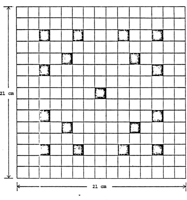
The PWR benchmark problem was designated CC3. A layout is shown on Fig. 1. The assemblies used (rodded or unrodded) are shown on Fig. 2. _{Two fuel enrichments (1 and 2) are present and one of the} assemblies contains a partially inserted control rod (shaded area in

Fig. 1, composed of 16 shaded regions - not the central one - of Fig. 2).

The other assemblies (non-fuel composition - 3) contain 17 water holes. The flux boundary conditions are as indicated.

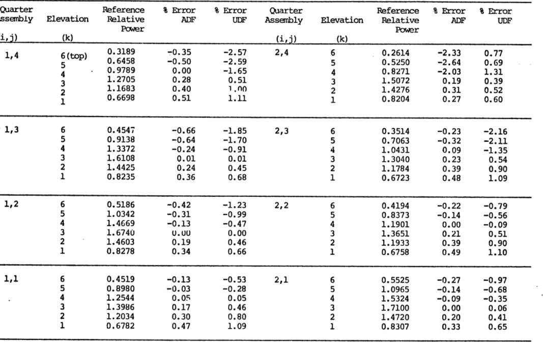
A 3D PDQ reference for this problem was provided by Northeast Utilities. _{Table 1 shows errors in nodal power as compared with this} reference. _{All axial discontinuity factors were taken as unity and radial} discontinuity factors were taken as either unity (UDF) or as those provided

-7-(LY) '2.0 3:L 4 r, I -J O 3j

10o.S

k

V5

20.0

0.0

21 cm

dimensions of each cell = 1.4 cm by 1.4 cm

Fig. 2 Heterogeneous PWR assembly geometry.

21 cm

--

I

I

Table 1: Nodal Pcwer Results for the Three-Dimensional CC3 Problem

Quarter Reference % Error % Error Quarter Reference % Error % Error

Assembly Elevation Relative ADF UDF Assembly Elevation Relative ADF UDF

Power Power (i,j) (k) (i,j) (k) 0.3189 -0.35 -2.57 2,4 6 0.2614 -2.33 0.77 1,4 6t) 0.6458 -0.50 -2.59 5 0.5250 -2.64 0.69 4 0.9789 0.00 -1.65 4 0.8271 -2.03 1.31 3 1.2705 0.28 0.51 3 1.5072 0.19 0.39 2 1.1683 0.40 1.n00 2 1.4276 0.31 0.52 1 0.6698 0.51 1.11 1 0.8204 0.27 0.60 1,3 6 0.4547 -0.66 -1.85 2,3 6 0.3514 -0.23 -2.16 5 0.9138 -0.64 -1.70 5 0.7063 -0.32 -2.11 4 1.3372 -0.24 -0.91 4 1.0431 0.09 -1.35 3 1.6108 0.01 0.01 3 1.3040 0.23 0.54 2 1.4425 0.24 0.45 2 1.1784 0.39 0.90 1 0.8235 0.36 0.68 1 0.6723 0.48 1.09 1,2 6 0.5186 -0.42 -1.23 2,2 6 0.4194 -0.22 -0.79 5 1.0342 -0.31 -0.99 5 0.8373 -0.14 -0.56 4 1.4669 -0.13 -0.47 4 1.1901 0.00 -0.09 3 1.6740 U.00 0.00 3 1.3651 0.21 0.51 2 1.4603 0.19 0.46 2 1.1933 0.39 0.90 1 0.8278 0.34 0.66 1 0.6758 0.49 1.10 1,1 6 0.4519 -0.13 -0.53 2,1 6 0.5525 -0.27 -0.97 5 0.8980 -0.03 -0.28 5 1.0965 -0.14 -0.68 4 1.2544 0.05 0.05 4 1.5324 -0.09 -0.35 3 1.3986 0.17 0.46 3 1.7100 0.00 0.06 2 1.2034 0.30 0.80 2 1.4720 0.20 0.41 1 0.6782 0.47 1.09 1 0.8307 0.33 0.65 __ ___ _. ___ ____~_ ~ii_ _~___C~_ __

by a 2D fine-mesh calculation run for the assembly with zero-current boundary conditions imposed (ADF). The ADF results are superior

everywhere except in the rodded portion. This result is consistent with previous 2D results, which show that color set determinations of discon-tinuity factors are superior to assembly calculations for rodded nodes. In any event the use of unity factors for the axial direction seems satis-factory.

The BWR benchmark problem (TRD) is shown on Fig. 3, the

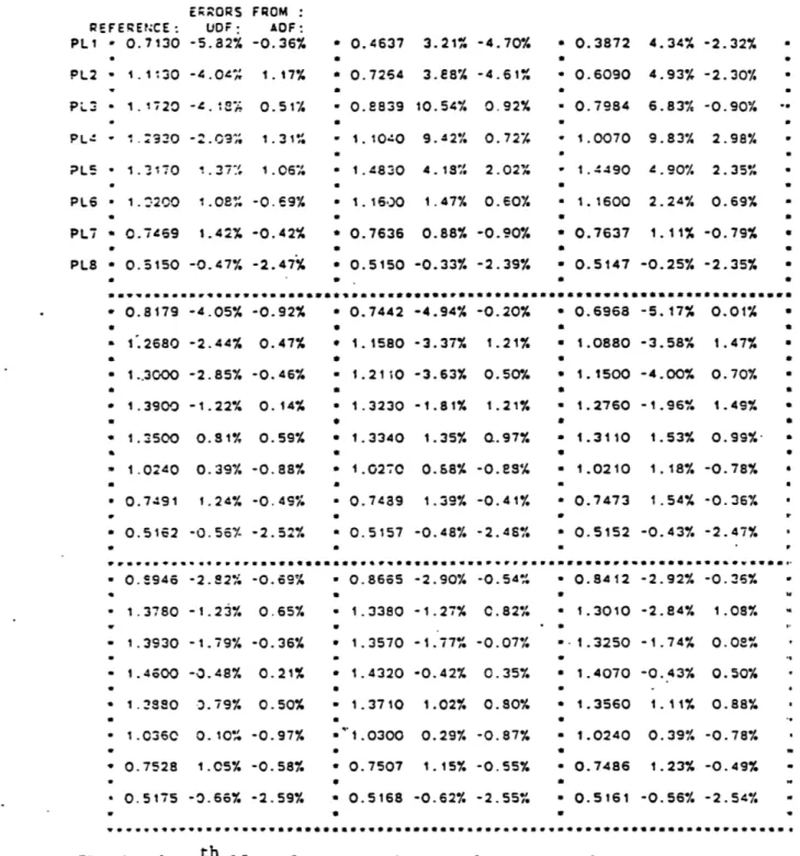
assembly geometry and assumed void distribution being shown on Figs. 4 and 5. Nodal powers (as edited from a fine-mesh, 3D, PDQ calculation provided by Northeast Utilities) and QUANDRY errors arising from the use of UDF's and ADF's are given by Table 2. Unity axial discontinuity factors were used in both cases.

Again the ADF's provide superior results except in the rodded nodes and adjacent to the top reflector. Since 2D results have shown this same behavior, we conclude again that the use of unity discontinuity factors for the axial direction is a legitimate approximation.

Both the CC3 and TRD benchmarks involve reflecting boundary

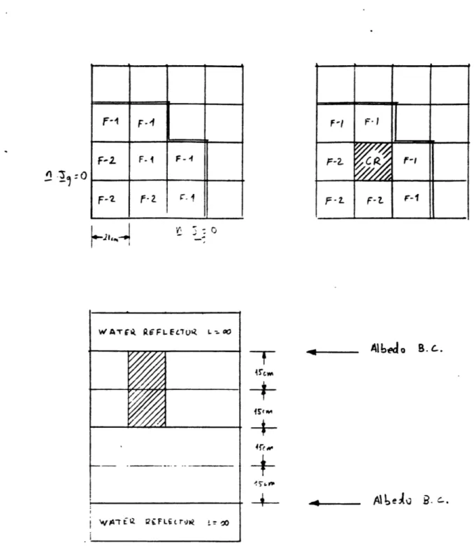
conditions in the radial plane. In order to determine whether the presence of a radial reflector invalidates the use of unity discontinuity factors for axial interfaces, we have analysed a small 3D benchmark problem which incorporates features of a PWR. The geometric characteristics of this benchmark (called the EPRI-9-3D problem) are shown on Fig. 6. The assemblies making up the reactor are of two enrichments (F-1 and F-2) and are geometrically those shown on Fig. 2. The sixteen control rod fingers (the shaded areas of Fig. 2, excluding the central one) are

-11-JN=0

15.31

I.

J, N=0

Figure 8: Radial Core Layout for the TRD BWR Benchmark Problem

REFLECTOR REGION 4

REGION

3

REGION 2

REGION 1

Axial Core Layout for the TRD BVR Benchmark Problem

20,00

30.00

15,00

15.00

30,00

30,00

20.00

77~

L~I

---~Xi""-- i -- I_- __ -~--a~_-- i .- .__1._- - -;...-;--- ; _---...r^-__---- __~a-m---~;i^_._~~_;--r ---_~

,,,,, ~ I.

-Figure 3:

I

II

Figure 4: Assembly Description for the TRD BWR Benchmark Problem 12.45

c

L

-13-REGION

1

REGION

2

REGION 3

4

Void Fractions for the TRD BWR Benchmark

V=70% V=40%

V=40%

V=70%

V=70%

V=70%

V=70% V=70% V=70%

V=70 % V=70% V=70%

V=70% V=70% V=70%

V=70% V=70% V=70%

E.RORS REFERENCE: UDF : PL1 " 0.7130 -5.a2% PL2 - 1.1130 -4.04%" PL3 1.17T20 -4. 1 . PL 0.2930 -2.09%; PL5 * 1.3170 1.37: PL6 * 1.2200 1.08% PL7 * 0.7469 1.42% PL8 * 0.5150 -0.47% * 0.8179 -4.05% a 1.2680 -2.44% * 1..3000 -2.85% * 1.3900 -1.22%. * 1.3500 0.81% - 1.0240 0.39% * 0.7491 1.24% • 0.5162 -0.56%-0.8946 1.3780 1.3930 1.4600 1.3880 1.0360 0.7528 0.5175 FROM : AOF: -0.36% 1. 17% 0.51% 1.31: 1.06,% -0.69% -0.42% -2.47% -0.92% 0.47% -0.46% 0.14% 0.59% -0.88% -0.49% -2.52% Q***w********* -2.82% -0.69% -1.23% 0.65% -1.79% -0.36% -0.48% 0.21% 3.79% 0.50% 0.10% -0.97% 1.05% -0.58% -0.66% -2.59% 0.4637 3.21% -4.70% 0.7264 3.E8% -4.61% 0.8839 10.54% 0.92% 1.1040 9.42% 0.72%, 1.4830 4.18% 2.02% 1.1600 1.47% 0.60% 0.7636 0.88% -0.90% 0.5150 -0.33% -2.39%

•** ago:* I**at* a**a

0.7442 -4.94% -0.20% 1.1580 -3.37% 1.21% 1.2110 -3.63% 0.50% 1.3230 -1.81% 1.21% 1.3340 1.35% 0.97% 1.0270 0.68% -0.88% 0.7489 1.39% -0.41% 0.5157 -0.48% -2.48% 0.8665 1.3380 1.3570 1.4320 1.3710 "1.0300 0.7507 0.5168 -2.90% -0.54% -1.27% 0.82% -1.77% -0.07% -0.42% 0.35% 1.02% 0.80% 0.29% -0.87% 1.15% -0.55% -0.62% -2.55% * 0.3872 * 0.6090 * 0.7984 * 1.0070 - 1.4490 a 1.1600 a 0.7637 S0.5147 *****ew** * 0.6968 a 1.0880 * 1.1500 * * 1.2760 a 1.3110 a 1.0210 a 0.7473 a 0.5152 * 0.8412 * 1.3010 8-1.3250 a 1.4070 * 1.3560 a 1.0240 * 0.7486 a 0.5161 4.34% -2.32% 4.93% -2.30% 6.83% -0.90% 9.83% 2.98% 4.90% 2.35% 2.24% 0.69% 1.11% -0.79% -0.25% -2.35% -5.17% 0.01% -3.58% 1.47% -4.00% 0.70% -1.96% 1.49% 1.53% 0.99%-1.18% -0.78% 1.54% -0.36% -0.43% -2.47% -2.92% -0.36% -2.84% 1.08% -1.74% 0.08% -0.43% 0.50% 1.11% 0.88% 0.39% -0.78% 1.23% -0.49% -0.56% -2.54% th

PLn is the th 15cm plane grouping. n=l1 corresponds to the bottom fueled slice of the core.

WATGik REFLETOU L-.0

I

-

E

2_FLi

cro

19

Fig. 6 The EPRI-9 3D Benchmark Problem.

EMWI Mlii -15-A 3:o0 Al

6edo

-+--F

±r_.

We have already mentioned that, for rodded nodes, radial discon-tinuity factors based on 2D fine-mesh assembly calculations with zero-current boundary conditions lead to errors in nodal power of several percent. Figures 7, 8 and 9 illustrate this situation. Figure 7 shows comparisons of QUANDRY and PDQ for the 2D unrodded slice of the EPRI-9-3D problem. All homogenized group cross sections and discon-tinuity factors for the fuel nodes (4 nodes per assembly) were computed from assembly calculations (indicated by "A" on the lower figure). Color set calculations involving quarter assembly nodes and neighboring baffle-. reflector nodes were used to determine homogenized cross sections and discontinuity factors for the nodes on the reflector side of the core-baffle interface (indicated by "C3" on the lower figure). The errors in nodal power are quite acceptable (< 0. 5%).

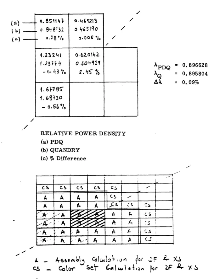
Figure 8 shows the results when the same procedure is applied to a rodded radial slice of the 3D benchmark. The error of 2. 45% in power for the rodded node is probably acceptable, but it is much greater than that in the unrodded nodes.

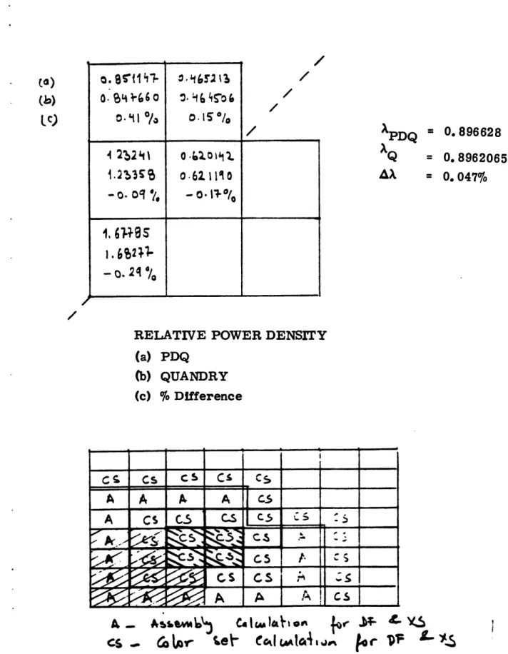
Figure 9 illustrates what happens if color set calculations are used to determine homogenized cross sections and discontinuity factors for the rodded slice. Errors in nodal power predictions as compared with PDQ are again < 0. 5%. Accordingly, in order to obscure as little as possible! errors due to use of unity-valued axial discontinuity factors,we have used for the 3D analysis radial parameters based on color set calculations for the rodded nodes.

On Fig. 10 the 3D QUANDRY predictions of nodal power are

com-pared with those edited from a two-group, fine-mesh (" 130, 000 mesh

-17-Fig. 7 _{EPRI-9 Problem - (D) (60 x 60 PDQ) No} (8 x 8) QUANDRY) - 1. -3J

Control Rod

RELATIVE POWER DENSITY (a) PDQ (b) QUANDRY (c) % Difference XPDQ

Q

J.

A * Assembly Calculation for DF & XS

CS Color Set Calculation for DF & XS

(.)

(c)

(C)

Fig. 8 EPRI-9 Problem - 2D - _{(60 x 60 PDQ) with Control Rod.}

(8 x 8 QUANDRY)

(Color Sets obtained with 1.4 cm mesh int.)

S'i8Bf32 o. 2

8 .1

S"

I. 6 -'8S

-

o.S6

%

RELATIVE POWER DENSITY

(a) PDQ (b) QUANDRY (c) % Difference >PDQ

SQ

Ax

4ssemot%

Cotor

X.Sg)I

-19-Fig. 9 EPRI-9 Problem - 2D - _{(60 x 60 PDQ Reference Solution)} (8 x 8 QUANDRY)

(Color Sets obtained with 1. 4 cm mesh int.)

Btl

r3

249

s

AX

C4 Igo\

)AV 1,,

C L-o t

et

vr-

-20-Fig. 10 EPRI-9 Problem - 3D - _{(61 x 61 x 35 PDQ)Relative Power Density} (8 x 8 QUANDRY) (a) (b) (c) PDQ QUANDRY % Difference 0. 10 (, 0o. 70q o. fo% 0. Sal f3% 4, O000 Q 45006 4, oo 54 0oq."61

-o.

2f

/

-

%.

olo

o.6G 6Soo.67- 68o 0.6"-46 O.Si%% PLAE" #* 3 0.84 4'3 PLANE # &X,=

O.

6/

/

> 9J4 =

(to ED)

-21-encouraging. The difference in eigenvalue is 0. 031%, and the maximum difference in nodal powers is 0. 71%.

These differences are less than those which occur if the PDQ mesh size in the radial plane is cut in half. This fact is illustrated in Fig. 11 which shows the 2D PDQ and QUANDRY results for the rodded plane when the radial mesh interval is taken to be 0. 7 cm rather than the 1. 4 cm used (for both PDQ and assembly-color-set calculations) to produce Figs. 7 to 10. Comparing the quarter-core PDQ results given in Figs. 9 and 11 shows that the difference in eigenvalue (due to mesh size alone) is 0. 075%, and the corresponding maximum difference in nodal power is 4. 6%. Presumably, roughly the same difference would be observed if a finer mesh 3D PDQ were run. However, Northeast Utilities could not get this larger problem (~ 500, 000 mesh points) to run on their IBM 3033 computer.

At present the preparation of the QUANDRY input must be done by hand; thus the manpower requirements to obtain the QUANDRY solution

are substantial. Machine CPU time expended is, however, small: about 20 seconds to run the required fine-mesh assembly and color set PDQ's, another 5 seconds to obtain discontinuity factors from the output and 8 seconds to run the final 3D QUANDRY solution. The CPU time for the PDQ was - 97 minutes. (All times are on an IBM 3033.)

IV. The Treatment of Partially Rodded Nodes

The test cases described in the previous section suggest that use of unity-valued discontinuity factors in the axial direction yields acceptably accurate results, provided there is a nodal interface at any location where there is a significant change in assembly characteristics, for example at the tip of a control rod. If a control rod is partially inserted in a node,

Fig. 11 EPRI-9 - 2D - (120 x 120 PDQ) with Control Rod Relative Power Density

(8 x 8 QUANDRY) n/ / / / o.9l3q'1 o. 417O86

o...

36

////

//

22?.

6502S'

(a) PDQ - Reference Solution (120 x 120) (b) QUANDRY Solution 8 x 3 Problem. (c) Relative Error in %.

XPDQ

xQ

= 0. 897297 % Error = 0.054%

= 0. 8968136

Shadowed area indicates where the control rod is inserted.

AXS and ADF have been obtained through color set calculations for nodes near the baffle and neighboring the control rod.

Assembly calculations have been performed for the other inner nodes.

(a)

(6)

(C)

i

i II O

-23-the radially homogenized cross sections for that node will change in a step fashion at the axial location of the tip of the rod, and it is quite unlikely that unity discontinuity factors at the axial faces of the node and simple volume weighted cross sections in its interior will lead to

accurate predictions of reactivity and nodal power distribution.

It is of course possible to circumvent this difficulty by requiring that there be a nodal interface plane positioned at every control rod tip. But if one is dealing with part-length or stuck rods or is performing a

search for the control rod bank position corresponding to the critical

condition, this procedure can become complicated - particularly if

power-dependent feedback effects (due to Xe, Sm, thermal-hydraulics, etc.) are

being accounted for. For reactor transients during which control rods

are moving, complications become even more severe. Thus there is

considerable motivation for locating axial nodal interfaces at fixed planes and dealing with the intra-node axial discontinuities associated with

partially inserted control rods by using some combination of non-unity axial discontinuity factors and/or axially flux weighted homogenized cross sections.

The September-April progress report showed that the use of discon-tinuity factors can get rid of the control rod cusping problem in QUANDRY

computations. The possibility of making use of tabulation-interpolation

methods was examined. However, the results of the investigation showed

that these methods are problem-dependent, require complete global

calculations, and demand considerable machine memory space - all

unattractive features.

Since that time we have found a simple systematic, problem-independent way to solve the cusping problem in QUANDRY using data

internal to the code. Results obtained using the new method have been compared with those of both the volume-weighted-cross section approxi-mation method and the quadratic axial flux shape approxiapproxi-mation currently programmed into QUANDRY. In view of the results described in the previous section, radially homogenized cross sections and discontinuity factors were assumed to have been found already, and reference solutions were finer mesh QUANDRY solutions.

For estimation of correct homogenized cross sections (XS) and axial discontinuity factors (DF) of a partially rodded node (PRN), an axial flux reconstruction method has been introduced. The purpose of the flux reconstruction is to predict (in a step called "Predictor") the axial flux shape within a PRN of the system of interest using information already

available from the same system and collected in another step called

"Collector". If predicted correctly, the XS and DF of a PRN thus obtained will yield the correct reactor solution for both static and transient

situations.

Actually two such methods have been examined. The first is relatively simple but, for some situations, somewhat inaccurate. The

second is more complicated but is capable of performing more accurate predictions adequate for transient calculations.

Method 1

This method makes use of the nodal flux shape information implicit in the QUANDRY solution for the case of the control rod tip positioned exactly at an axial nodal interface. Two adjacent nodes, one fully rodded (r) and the other completely unrodded (u) (see Fig. 12(A) are

solved for the one-dimensional axial flux shapes within them, with

-25-A.

M

ETHOD

_

TRWJ

- . METHOD

Z

C

PRw

Fig. 12 The Collector-Predictor Methods. I _ _ I

the global QUANDRY solution. Transverse leakage terms can be approxi-mated as quadratic in shape. Then the axial flux shapes for the two nodes are displaced (see Fig. 12(A)) to construct an approximate flux shape within the partially rodded node (PRN). With this new flux shape, one can calculate

FWC. These homogenized cross sections and the surface currents at the axial faces of the PRN region (lower portion of Fig. 12(A)) can be used to calculate hom, surface Thus the discontinuity factors f for the PRN can be found.

In addition to homogenized cross sections and axial discontinuity factors for the PRN, one needs to know radial discontinuity factors.

Fortunately, without any supplemental calculation, the radial DF's can be estimated by making use of the volume-averaged fluxes r, PRN and

u PRNC)

(huPRN for the two regions of a PRN (A' and B' in Fig. 12). Derivation of

(h) +

this approximation is sketched on Fig. 13 for the surface x . Many test results have shown that this approximation is acceptable (accuracy greater than 99. 0% for most radial D. F. estimations of a PRN).

The basic assumption of this first method is that the axial flux

shapes around the control rod tip do not vary significantly when the control rod travels the distance of one axial node.

Method 2

To improve Method 1, we make use of the flux shape already constructed for a previous partially rodded condition. Thus the shape between the dotted lines in the upper portion of Fig. 12(B) is translated and assumed to be valid in the lower PRN region. Thus we solve (analytically) a one-dimensional, three-region problem for axial flux shapes throughout regions U, A, and B. Then we edit out the axial flux shape appropriate to the altered control rod tip position (lower portion of

- - ~- --- -- --- III~u

-27-rfi (+;

W,

*h

WEv

---

,4

4) X'

I rw

_V+

r,

T's 4x4

9,I4

kr,

u, PQI

v

crPR

Pbrt

Fig. 13 _{Radial Discontinuity Factors for the Partially Rodded Node.}

+rwo

kc~

Fig. 12(B)). For a displacement shorter than the axial node size, this second method will predict more accurate homogenization parameters than Method 1. It is particularly useful for transient rod withdrawal problems.

The Collector-Predictor methods, along with the conventional

volume weighted cross section (VWC) and quadratic axial flux approxima-tion methods were tested and the results were compared for the CC3-PWR

and TRD-BWR bench mark problems described in section III of this report. However, to avoid the errors discussed earlier arising from use of

isolated assembly calculations to compute radially homogenized cross sections and discontinuity factors, two-dimensional calculations for full planes were done to obtain the radial AXS and DF's for nodes in different kinds of planes. Thus, errors due to the use of AXS and ADF from single, isolated assembly calculations were not present in the test problems.

For the CC3-PWR model (see Fig. 1 ) static tests were performed for the tip of the control rod located at 11 positions ranging from the 85 cm to the 138 cm axial location (see Fig. 1 ). As mentioned above, radially homogenized nodal cross sections and discontinuity factors were found from full planar, fine-mesh calculations with all water hole and control rod heterogeneities represented explicitly. Three-dimensional QUANDRY

problems making use of the resultant AXS's and DF's, and with an extra axial plane inserted at the location of the tip of the control rod in the PRN, were taken as numerical standards (unity valued axial discontinuity factors were assumed for these standard calculations). Eigenvalues and power distributions as computed by Method 1 and by the conventional volume weighted cross section method (VWC-axial discontinuity factors unity and

v V

PRN homogenized cross sections given by P" RN Vr r + u u

v +v v +v

r u r U

-29-Table 3 and Fig. 14. Clearly Method 1 is far superior to the VWC scheme. The rod cusping effect can be seen to be present for the VWC results but absent when Method 1 is used. The same CC3-PWR model was used for transient tests. The control rod was withdrawn for 0. 1 sec from the 100 cm to the 120 cm position. The withdrawal was accomplished in ten time steps. The results are shown in Table 4 and Figs. 15 and 16. The predictions of both Method 1 and Method 2, along with VWC and the quadratic axial flux method programmed into QUANDRY (axial f's = 1; axial flux shape in the PRN a quadratic fit to the average flux levels in that node and its two axial neighbors), were compared with the standard, which used unity axial discontinuity factors but had a sufficient number of axial planes that the control rod tip was on an axial plane at each time step.

The results show that both Methods 1 and 2 are much more accurate than the VWC or quadratic axial flux schemes. Since the cost is only marginally greater, Method 2 (the most accurate) is favored.

A similar study was performed for the TRD-BWR model specified by Figs. 3 to 5. Static results for the rod fixed at various locations

in an internal axial node and in an axial node next to the reflector are displayed in Figs. 17 and 18. Table 5 provides the numerical data. The

acceptability of Method 1 as well as its superiority to the convensional VWC method is again demonstrated.

Figures 19 and 20 display the results of a rod withdrawal transient for the TRD-BWR. The withdrawal rate from the initial critical position

was taken to be 300 cm/sec, and the transient was followed for 0.04

seconds. The inadequacy of the VWC model and the remarkable accuracy of the two new methods - particularly Method 2 - is again evident.

We believe that these results demonstrate that Method 2 provides a

Table 3

Comparison of keff and Max. Nodal Power Error of CC3-PWR Model (Static Problem)

ME-O

PDL

c.R.

TiP

PD

TI

C.,?'

~,5.

f

0.

L9.

L

/00.1

*

I

//0.

///.

/2.

/3S.

/ 38.

RFECRUCE

;I x 4x'

0.

q~yq3

o,

qSorz

o.

9 336

vW ..

- o. o6S

%

-.

# ly

S-o.

039

---.

M0

o

81

-o.

o S-r

yo%

:

-o. os/

-o.

-3.

₃

0.

95 3

_--

-o.o

_S'S,

_{_%}

.

_{-o.o. .}

a7

o

--

0

,

,0

--

-I. ?

-O.2'

4~

-o.qoo?

-

0.0027

-1, A7 a

-0.'9%

II

i1

I

-o. o#

fo

.3

i

4

o0 .

1

S9

-31-REFEReJCE , 2 X XA

nodes

CI

TmoD,

A

2 X 4

nodes

VWC

, 24)(1 nodes

CORE

CONTRoL RVOP -nP

FUL

rIP-POINT

POSI

lIP-PO'IAT

P&sITIPN (C)

TOP

Fig. 14 Comparisons of keff and Nodal Power for CC3-PWR. ' ~'IIIIIIYYI~ ~~II i

Table 4

CC3-PWR Transient Due to C. R. Withdrawal (Total reactor power in watts, and

%o

METH0P

REFCEUECE

VWC

fUAUPhATIC

_METHOD

_METODA

mll

IMt

I L

F 4Aj

TIP

Xsm

x4xlq

xt

.8

'x 2.Xx4A

AxL4xjt

57ITS AT /00 -cr 00 W /O0 V /00 I /0o 0 /0 .w

lo3,

76

o

e

1y6

od

0d4. 6

/,.

7

// /. 66

/

t. '2

1 d

17._u .

" --.

",

/./5

% ,-o.

S

%

8

9

I1.

/l;.

1

/o..

Y

_,

/_.o

/.,(

9

_-.

_-

_/

_q

_{/ .}

/.2'.

2

/.o-

/

I;A

1 1 %3 1

3/

.

_.

₃

-q./

%

-/ 9,

--

i3.1

-oA' 7,

S/2

1. 71

_-/3.

₄

_-'..

_%

_,-3.6

_.

_L

_-

_,7

/Ao.

3

03z

2.

73

_/.6

_:/.

/ /

4.

// /? 29.

2$-. ff

0

_logO,

_Om

_{/). X, 0.32}

_OP/

i

_.2.

_/

_,236

6

?-73 Yo

-.

377, --z,

7

o3

23.

o

76

i

I

- ~II U I1h -33-SMETOD / Total / • Power tC At/ /

WC

.X,

//X

8

I/

c.

ait

//0.

/

P77

2.

C'ONT'DrL RD TiP posl0/74J

Fig. 15 Total Power Transition of CC3-PWR.

--2P.

VWC

.x

jXg

/A///

CowRtOL

O

/P

PsmNo4

,---*

to en

Fig. 16 Total Power Error in Transition of CC3-PWR.

Table 5

Comparison of k pf and Max. Nodal Power for Static TRD-BWR Problems

I

I

iaLbu'

oW

0, 40 Y

_0,

4'oX

So.o

o(V

VOD TPlACTIO) OF cooLA

T

w* DIlRECMOW OF ROp MOVEMENT

o.176

VWWC- ,

3xxblo

. -

-

M

X.

COaTRo.. 0 AD&E

TIP-POITIONIV

(Cm)

Fig. 17 Configuration and Comparisons of keff and Nodal Power Error for Rod at Various Axial Positions in a Central Node.

121F. 110. 95. l.

_,s~

so.

Itor

. 9qt

J

,= 0.,

r7 9

S ,-a

O.,

4D

0

o.4979

-*-REZeR-JCE

,

gA( A3

*TT ,

3A 3( 10

MIN.

A*VVL

POWE- eWOR

(%)

ev

S= P)IRNECTIOW

OF ROP mcVEMEOt

r

5Ac.

CONTROL 1O9DE TIP

POSTIOv

( C-rr)

Fig. 18 Configuration and Comparisons of keff and Nodal Power Error for Rod at Various Axial Positions in a Node Adjacent to the Bottom Reflector.

4,

da r

_65'.

3S&

*

a

o 4,

0

VOID FMATPlo,

oF coOL ,AT

.-

) = DIRECTIO

_{OF RDE MDPVEP)rET.}

Fig. 19 Axial Layout and Numerical Results for the TRD-BWR Rod Withdrawal Transient.

PDITIo 3

x

3

-

6SCii

100. /

10oo.

100.

/

(oo.

W

14.

02

.

7-

/.2##23.

72.

-

-2o, 7 g

.87%

,o. 13 %

______

-/,A.%

-o.4

4,

-o.

d

.394/

.

o3 .

3o3

J. ISr

435$. 3

.

666. 6/ -7/.

3/

- 33s

-323

d

t/ A/

i/O.

~0o

69.

o4J

A0T'T//~

-39-pp- REFERJECE . 3X3x1if --- -- METHOD

a

-

VW.

, 3x 3Xto

6o0.

3oo.

300.

.oo.

6.O

i..

s

s.

3.

Control Blade Tip Position (cm) (rod moves 3 cm every 10 ms)

Fig. 20 Total Power vs Control Rod Position During Transient.

f0o.

o0.

satisfactory resolution of the rod cusping problem for the QUANDRY code. The scheme can be applied simply and automatically entirely within the framework of the QUANDRY equations using data already

generated during normal operation of the code. It is cheap to implement and appears to yield, consistently, very accurate results.

V. Reconstruction of Fine Mesh 3D Flux Shapes from Nodal Solutions

In the September-April progress report we summarized tests of methods for reconstructing local fuel pin power from two-dimensional nodal solutions. The tests were for two-dimensional PWR and BWR benchmark problems depleted up to the beginning of a third fuel cycle with fuel shuffling and assembly rotation taking place between cycles. The basic assumption underlying this reconstruction is that the flux within a given heterogeneous node or on the nodal surfaces can be

expressed as the product of a biquadratic polynomial (a "form function") multiplied by a fine-mesh "assembly" flux shape which reflects the detailed heterogeneous nature of the fuel assembly. For the PWR test case, assembly shapes using zero-current boundary conditions were sufficient to give maximum pin power errors of less than 5% for all the depletion steps. (Maximum error in the "hot" pin was 1. 02%.)

For BWR's this simple approach led to fuel assembly power errors as great as 5. 19%, and it was necessary to use an iterative response matrix approach to obtain accurate assembly powers and then an extended assembly scheme to obtain maximum fuel pin powers of under 5%.

This response matrix approach, while successful, is expensive (chiefly because of the cost of generating response matrices) and looks foreboding if extended to three dimensions. However, the PWR scheme

-41-is relatively straightforward and appears to be acceptably accurate. Accordingly we have extended it to the 3D-PWR benchmark shown in Fig. 6.

Determining the quadratic form function from the nodal solution is necessary for both the PWR and BWR reconstruction procedures. Both require that corner point flux values be inferred from the nodal results. In two dimensions the assumption that the form function is quadratic on the mesh lines connecting corner points along with values of the average fluxes along these lines found from the nodal solution is sufficient to determine the corner point values. However, in 3D, the line-averaged fluxes must themselves be inferred from the nodal solution. Accordingly, before presenting numerical results we shall sketch the overall theory of reconstructing detailed flux shapes using the output of nodal calculations along with fine-mesh fluxes found from zero-current assembly (or color set) calculations for the heterogeneous node of interest.

The basic assumption we make in order to perform a 3D fine-mesh flux reconstruction is that for each group, g, and within any node (i, j, k)

ijk

the reconstructed flux, _gk (x, y, z), can be expressed as the product of an assembly function, O j (x, y), and a triquadratic polynomial function,

g

k (x, Y,z) = (x, y) Pijk (x,y,z) (g= 1,2) (1)

g g g

where

(x, y, z) is a point in node (ijk);

0k (x, y, z) = unknown reconstructed flux; g

Oj (x, y) = known assembly flux; g

pijk (x, y, z): tri-quadratic polynomial in x, y, and z g

with 27 unknown coefficients.

The assembly flux $~ (x,y) is obtained by performing a fine-mesh, g

2D flux calculation (a PDQ zero-current assembly or color set calculation). The polynomial function can be written as:

pijk (x,y,z) = l m n (g = 1,2)

P (xz)m _{1=0 m=0 n=}n ag; , m,n *y z

(2) Note that separability is not assumed for this function. Thus there are 27 independent polynomial coefficients.

Once these "a" coefficients are found, and auxiliary color set cal-culations have been performed, one can compute the flux in any point within node (ijk). Thus the major problem consists of finding such

poly-nomial coefficients. In order to find the polynomial coefficients it is first required that the reconstructed flux, (R' when integrated over the nodal

surfaces and the nodal volume, shall reproduce the nodal averaged values, which are obtained through a 3-D QUANDRY solution.

Thus, so far, we have a system of 27 unknowns (for each group and node) and a set of 7 equations (6 for the nodal surfaces and 1 for the node volume). To determine the "a" coefficients we need to find an additional set of 20 equations. This additional set of equations can be

obtained by forcing the reconstructed flux gijk (x, z) to satisfy the 2-group Rg

Neutron Diffusion equations about nodal corner points, and by forcing the reconstructed flux to satisfy, in an integral sense, the 2-group Neutron Diffusion equations along nodal lines.

Thus we get one independent equation for each nodal corner point and one independent equation for each nodal line. Since there are 8 nodal

-43-corner points and 12 nodal lines, the number of balance equations per node is 20.

Thus we have (per group and node) a system of 27 equations: 7 obtained matching the nodal solution and 20 derived by satisfying the two-group neutron diffusion equations about corner points and along nodal lines. We can solve this system for the 27 unknown polynomial

coefficients, and thus reconstruct the flux by using Equation (1).

By rewriting the polynomial function, p, appearing in Equation (2), and introducing a proper set of known "integral coefficients", which depend on the node geometry and assembly flux, it is possible to express this polynomial explicitly in terms of the 8 unknown corner point fluxes and 12 unknown line averaged fluxes, and in terms of the known surface averaged and volume averaged nodal values.

By doing this, we transform a general tri-quadratic polynomial, P, with 27 unknown coefficients into an equivalent polynomial, Q, with only 20 unknown coefficients (the surface averaged and volume averaged fluxes being known from the QUANDRY solution).

The reconstructed flux, expressed in terms of Q, becomes:

k (x, y, z) = 1ij (x,y) - Qijk (x,y,z) (3)

Rg g g

where the coefficients of Qijk are such that _{g Rg}jk will reproduce the (still unknown) corner point fluxes, c' and line averaged fluxes, (L as well as the (known) face averaged and volume averaged nodal fluxes.

The polynomial function Q k is an analytical function and thus continuous and differentiable within the node. However, the assembly function

41

equation by a finite difference approach. Thus it is neither continuous nor differentiable within the node.

In order to be consistent mathematically, it is convenient to treat the polynomial function as piecewise flat within mesh cubes, rather than as an analytical function, and then to solve the two-group finite difference neutron diffusion equations, rather than the two-group partial differential equations.

With this understanding we force the reconstructed flux to satisfy the two-group neutron balance equation about node corner points and along node lines in a finite different fashion.

First, the 3D reactor is divided into large nodes; then at any corner point (ijk) one can set the following system of equations:

1. Balance equation around corner point (i, j, k). 2. Balance equation along the node line parallel to x. 3. Balance equation along the node line parallel to y. 4. Balance equation along the node line parallel to z.

Since the reconstructed flux is expressed in terms of the unknown corner point fluxes and averaged fluxes along lines, then, the implementation of these equations at all node corner points will result in a system of

coupled linear equations relating all corner point fluxes and averaged line fluxes. Since the coupling is very strong, and since both groups are coupled, one needs to solve the system of linear equations simultaneously by an iterative scheme.

In order to express a mesh point balance condition about corner point I, J, K we first note that, for mesh-point-centered difference

equations (those used by PDQ), there will be a number of fine-mesh points between one corner point and the next, and the finite difference balance condition about that corner point will relate the group-g flux QI J, K at

gthat corner point to the group-g fluxes of its six nearest "fine-mesh"

-45-neighbors and to the other group flux at (I, J, K). But the nearest "fine-mesh" neighbors all lie on lines connecting (I,J, K) to its six

nearest "corner-point" neighbors I±1, J, K), (I, J±l, K) and (I, J, IKl), and the flux shape along the line connecting, for example, corner point I, J, K to corner point I+1,J,K is being expressed as a product of the (known) assembly shape and a quadratic form function shape, which in turn is specified by g, J, K, +1,J, K and +1, J, K , the average group-g flux

eg cg gx

along the line connecting I, J, K to I+1, J, K. Thus the "fine-mesh" flux

nearest to I, J, K can be expressed as a linear function of eI, J, K

g

I+1, J, K, and +1, J, K _{Analogous expressions can be found for the}

cg gx

other five "fine-mesh" fluxes nearest to I, J, K. Thus the finite difference balance condition for the mesh boxes surrounding a corner point connects

I, J, K to its six nearest neighboring corner-point fluxes, the six line-cg

averaged fluxes between I, J, K and the nearest "corner-point" neighbor, and the flux for the other group at I, J, K.

In an analogous fashion the unknown line-averaged flux +1,J,K gx between I, J, K and I+1, J,K can be coupled to its four nearest parallel, line-averaged, "fine-mesh" fluxes, and these in turn (because of the

assumed form of Equation (5)) can be expressed algebraically in terms of the four nearest (unknown) parallel "node-line-averaged fluxes"

+1, J+-il, K i+l, J, Ktl

SI+,J1K +1 , the (known) face-averaged fluxes on the four

gx gx

planes connecting the node-line I, J, K - I+1, J, K to its nearest parallel neighboring node-lines and the ten corner point fluxes I, J, K + 1,J,K

I, Jl, K I+1, Jil, K I+1, J,I and , J,gc

gc gc gc gc

Thus there are equations coupling each corner point flux and each line-averaged flux between corner points to other nearest neighbor corner

point and line-averaged fluosE and to the (known) face averaged and volume averaged nodal fluxes.

A computer program solving for all these unknowns has been written and found to be very fast-running. We have applied it to finding corner point fluxes for the EPRI-9 3D benchmark problem shown in Fig. 6. Recall that the assemblies comprising this benchmark have the

geometry shown in Fig. 2. It is the pin power at any location in these assemblies which we wish to reconstruct. The fluxes which give rise to that local power will be those specified by Eq. (3), where the iJ (x, y)

are known, two-dimensional fine-mesh shapes determined by assembly or color set calculations. Figures 8 and 9 show for the unrodded and

rodded radial slices of Fig. 6 whether the 4 ix, y) for particular nodes were taken from an assembly or a color set calculation. Recall that we use four nodes per assembly in the radial plane for these calculations. Also note that we have extended color set calculations into the baffle-reflector regions, although we have not used the information generated by such calculations for the core region.

Since the "fine-structure" shapes $1 (x, y) of Eq. (3) are taken g

from two-dimensional assembly or color set calculations, all reconstructed spatial shapes in the z-direction must be accounted for by the tri-quadratic functions Qijk(x, y, z). Thus at any fixed radial location (fixed x and y) the

z-dependence of c (x, y, z) will be represented as quadratic. However,

Rg

because albedoe boundary conditions imposed at the axial surfaces of the reactor were taken to represent an infinite water reflector, the thermal flux inside the reactor near these axial surfaces falls off exponentially. As a result, representing the z-shape of the thermal flux as quadratic in

the upper and lower 15 cm-sized nodes of Fig. 6 leads to severe (, 19%) errors in reconstructed corner point fluxes in the axial surfaces of the reactor core. (Note, however, that since QUANDRY implicitly accounts

-47-for the exponential behavior, the average nodal powers - see Fig. 10 -are in excellent agreement with the fine-mesh 3D PDQ result.)

Using a zero-flux boundary condition at the core-reflector inter-face would probably get rid of this difficulty. However, since an albedoe boundary condition is more realistic and since the reference 3D PDQ has been run subject to such a condition, we chose to overcome the difficulty by adding extra nodes, two-centimeters thick, on the core-side of the axial core-reflector interfaces. Thus for reconstruction purposes we reran QUANDRY maintaining the radial mesh layouts of Figs. 7 and 9, but with the axial mesh spacings shown on Fig. 21. Assuming that the

axial mesh shape can be represented by a quadratic in the 2 cm intervals next to the top and bottom reflectors and then by another quadratic in the 13 cm thick adjacent mesh intervals is far more accurate than assuming a single quadratic shape throughout the entire 15 cm intervals.

Previous calculations for two-dimensional cases have shown that the maximum error in the detailed, heterogeneous fluxes reconstructed throughout a node according to the two-dimensional counterpoint of

Eq. (3) always occurs at the corner points. Accordingly, a good measure of the accuracy of our reconstruction procedure are the errors in

predicted fluxes incurred at corner points. These errors are shown for the 3D EPRI-9 problem in Figs. 22 and 23. As can be seen, the

maxi-mum errors ( 7. 5%) occur on the radial periphery of the top and bottom planes where the fluxes are quite low. For all interior corner points

(including those on the top and bottom axial interfaces) errors are less than one per cent. At the corner points of the highest-power node (the

central node between planes 4 and 51 the corner point fluxes match the fine mesh PDQ results to better than 0. 3%. Such agreement with a full