HAL Id: hal-01878242
https://hal.archives-ouvertes.fr/hal-01878242
Submitted on 20 Sep 2018
HAL is a multi-disciplinary open access
archive for the deposit and dissemination of
sci-entific research documents, whether they are
pub-lished or not. The documents may come from
teaching and research institutions in France or
abroad, or from public or private research centers.
L’archive ouverte pluridisciplinaire HAL, est
destinée au dépôt et à la diffusion de documents
scientifiques de niveau recherche, publiés ou non,
émanant des établissements d’enseignement et de
recherche français ou étrangers, des laboratoires
publics ou privés.
Experimental validation of transient source term in
porosity-based shallow water models
Vincent Guinot, Sandra Soares-Frazão, Carole Delenne
To cite this version:
Vincent Guinot, Sandra Soares-Frazão, Carole Delenne. Experimental validation of transient source
term in porosity-based shallow water models. River Flow 2018 - Ninth International Conference on
Fluvial Hydraulics, Sep 2018, Villeurbanne, France. �hal-01878242�
Experimental validation of transient source term
in porosity-based shallow water models
Vincent Guinot1,2, Sandra Soares-Frazão3, and Carole Delenne1,2 1HydroSciences Montpellier, Univ. Montpellier, CNRS, IRD, Montpellier, France 2Inria Lemon, Inria, Montpellier, France
3Institute of Mechanics, Materials and Civil Engineering, Université catholique de Louvain, Belgium
Abstract. Porosity-based shallow water models for the simulation of urban
floods incorporate additional energy dissipation terms compared to the usual two-dimensional shallow water equations. These terms account for head losses stemming from building drag. They are usually modelled using turbulence-based equations of state (drag proportional to the squared velocity). However, refined numerical simulations of wave propagation in periodic urban layouts indicate that such drag models do not suffice to reproduce energy dissipation properly. Correct wave propagation speeds, energy dissipation rates and flow fields are obtained by incorporating a new type of source term, active only under transient situations involving positive waves. This source term does not take the form of an equation of state. It can be modelled as an artificial increase in water inertia. In this communication, an experimental validation of this source term model is presented by means of new dam-break flow experiments in idealized, periodic urban layouts. The experimental results validate both the existence and the proposed formulation of this new source term.
1. Introduction
Shallow water models with porosity for modelling shallow flows over complex topography and within complex geometry have become increasingly popular. Since the inception of the porosity approach [1, 2], a number of versions of porosity-based shallow water models have been derived and applied to urban flood modelling. The most widely used approaches to date are the Single Porosity (SP) model [3, 4] and the Integral Porosity (IP) / Dual Integral Porosity (DIP) model [5–7]. For both the SP and IP approaches, substantial effort has been devoted over the past years to the development of accurate momentum source term models. In the field of urban flood modelling, a key issue is the development of models for the drag forces induced by buildings. Anisotropy is a salient feature of the urban environment, with main streets and building alignment inducing preferential directions from both a geometric and hydraulic point of view. Such anisotropy should be reflected in the drag model.
So far, although many different models have been proposed in the literature [5, 7–9], discriminating between them has proved not to be an easy task. Most validations consist of either comparisons with laboratory experiments or validation of a numerical/analytical solution against refined flow simulations [4, 8–12]. The former often have the drawback that the domain under investigation is too small to offer meaningful and accurate statistics. The latter have the inconvenience that the refined flow solution has not been compared to real-world flows. Therefore, while the numerical approach allows one to assess the validity of the porosity model as an upscaled version of a refined model, it does not provide any information as to whether both models provide a faithful picture of reality. The present communication
aims to bridge the gap between these two approaches, by providing a coupled analysis of refined flow simulations and the simulation results of the DIP model. The DIP model is retained for several reasons. Firstly, it has proved noticeably more accurate than the SP and IP models in reproducing transients in idealized building layouts [7, 11, 12]. Secondly, the DIP model uses a novel momentum source term model, that yields unusual wave propagation properties [7]. This model has not been validated experimentally to date. The DIP transient source term model allows the self-similar character of the flow solution to be preserved when applied to Riemann problems such as the urban dam-break problem, while usual momentum source term models do not. While the self-similar nature of the solution of the Riemann problem is known from pore scale-averaged refined flow simulations [7, 12, 13], no experimental evidence is available for it. Confirming the self-similar nature of the flow solution of the urban dam-break problem experimentally is thus of salient importance to discriminate between the various source term models proposed in the literature.
The present paper is organized as follows. Section 2 recalls briefly the governing equations of the DIP model. The experimental setup used for the validation is described in Section 3. The results are presented and discussed in Section 4. Section 5 is devoted to concluding remarks.
2. Dual Integral Porosity (DIP) model
The one-dimensional restrictions of the shallow water model and the DIP model [7] have a common differential vector writing in conservation form
tu
I M
xf u s (1a)
,
, , 2 2 2 , 0, 2 T T T x g h hu hu hu h s u f s (1b)
0
x f D s g h S S C h u u (1c) 0 if 0 0 0 , 1 if 0 0 t t h h M (1d)where u, f and s are respectively the conserved variable, flux and source term vectors, I and
M are respectively the identity and momentum dissipation matrices, CD is the building drag coefficient per unit depth, g is the gravitational acceleration, h is the water depth, S0 and Sf are respectively the bottom slope and bottom friction slope, u is the x-flow velocity, and are respectively the storage and connectivity porosity, and is a dimensionless coefficient between 0 and 1 accounting for momentum dissipation. The shallow water equations are obtained as a particular case of the DIP model by setting = = 1 and CD = = 0 in equations (1a-b).
Drag coefficient-based models of building drag were introduced in the IP model [5]. Originally, the approach used an isotropic coefficient CD. More refined drag models have been introduced since then to account for anisotropy effects stemming from building alignment: in the DIP model, a 2×2 tensor formulation for CD is used [7], an approach generalized in [9], with the tensor formulation as a particular case. A more complex and general, fourth-order tensor formulation had been proposed in [8]. However, in one dimension of space, all these approaches simplify to the same formula, with a single drag coefficient, hence equation (1c).
A rather unusual term in the governing equations is introduced by the momentum dissipation operator M in equation (1a). As indicated by the multiplier in equation (1d), the momentum dissipation mechanism is active only when the water level is rising. This
particular behaviour stems directly from the underlying assumptions of the momentum dissipation model introduced in [7]. Momentum dissipation is assumed to stem from the multiple reflections of positive waves onto the building walls. Positive waves are present only when the flow domain is filling, hence the condition on the time derivative of the water depth for in equation (1d). Compared to more usual momentum source terms, the momentum dissipation operator (1a, 1d) induces a number of differences in terms of model behaviour. To start with, M modifies the flux vector, while classical momentum source terms do not. As a consequence, the hyperbolic character of the model is preserved. When active, the momentum dissipation coefficient acts directly on the wave propagation speeds of the solutions, while usual friction or drag terms have only an indirect action [14]. A third feature is that the wave propagation speeds depend on the flow dynamics, in that rising and falling water levels do not yield the same propagation speeds. In other words, the wave propagation properties of the model do not obey an equation of state. A fourth key feature of this model is that it preserves the self-similar nature of the flow solutions when Riemann, Initial Value Problems (IVPs) are solved, while drag-based models do not.
The momentum dissipation operator has been shown to be much more efficient than usual drag models in reproducing refined shallow water simulations of transient propagation in periodic building layouts [7, 12]. However, while this model has been validated in [7, 12] against refined numerical simulations using the standard shallow water equations, no experimental evidence has been provided so far for its validity.
3. Experimental setup and results
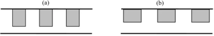
A scale model of an idealized street network was built at the Hydraulics Laboratory of iMMC. A series of periodic secondary streets making straight angles with a main street was obtained by placing 50 cm×75 cm rectangular blocks into a 20 m long and 1 m wide rectangular channel (Figure 1). The blocks were placed against the left-hand wall of the channel, the right-hand wall of the channel representing the symmetry axis of the main street. Changing the orientation and spacing of the blocks allowed different storage and connectivity porosities to be obtained. Configuration 1 (Fig. 1a), with a main street width of 25 cm and a longitudinal spacing of 50 cm, yields storage and connectivity porosities (f, f) = (5/8, 1/4). Configuration 2 (Fig. 1b), with a main street width of 50 cm and a block spacing of 50 cm, gives (, ) = (7/10, 1/2). An urban dam-break problem [13] was simulated by setting the water level to a predefined value hL on the upstream side of a gate, that was released within less than 0.5 s to simulate the instantaneous disappearance of the dam. For Configuration 1, there are respectively 9 and 12 block periods on the upstream and downstream sides of the dam. For Configuration 2, the number of upstream and downstream periods are 7 and 8 respectively.
Fig. 1. Bird’s eye view of the scale model of periodic, orthogonal street network. (a) Configuration 1:
longer block axis perpendicular to main street . (b) Configuration 2: longer block axis parallel to main street.
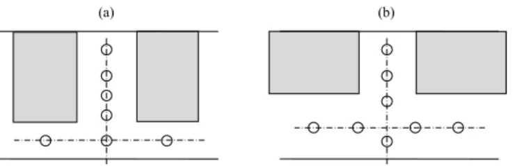
The water levels were measured in each of the block periods using ultrasonic probes, with an acquisition period of 0.2s. Figure 2 shows the locations of the probes for the two
configurations. Note that the interblock space where the gate is located was not measured because no room was available for the probes there. The water levels measured by the probes were averaged over every block period in view of the comparison with the porosity model simulation results. It is stressed that the water levels were not measured simultaneously over the entire scale model. Since only three probes could be operated simultaneously along a given transect, collecting the water level time series over a given block period required two to three replicates of the dam-break experiment. Moreover, in order to assess experimental uncertainty, each dam-break was replicated. In total, more than 300 experimental runs were needed to cover the entire scale model. Considering that each replicate requires 5 to 10 minutes to settle the initial conditions and carry out the transient experiment, approximately 10 working days involving two to four persons were necessary.
Fig. 2. Probe locations within each block period. Definition sketch for Configuration 1 (a) and
Configuration 2 (b).
The upstream water level hL was set to 0.35m. The transient phase was recorded over 30 s, which is beyond the time needed by the dam-break wave to cover the entire length of the scale model. In treating the experimental results, an experimental uncertainty t = ± 0.2 s and h = ± 1 cm was assumed from the water level time series recorded by the probes. Indeed, some of the probes recorded and initial depth of –1.5 cm at points where the bed was known to be dry. Moreover, oscillations with an amplitude up to 1.5 cm were observed in the upstream part of the experimental device during the filling phase.
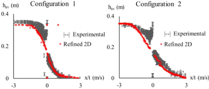
Figure 3 shows the block-averaged water depth hav as a function of x/t for Configurations 1 (left) and 2 (right).
Fig. 3. Experimental results. Block-averaged water depths for the two configurations. 0 0.2 0.4 -3 0 3 hav(m) x/t (m/s) Configuration 1 0 0.2 0.4 -3 0 3 hav(m) x/t (m/s) Configuration 2 (a) (b)
Clearly, the experimental values gather around an S-shaped curve. The few exceptions around x/t = 0 concern the closest probes to the moving gates. They may be attributed to wrong measurements resulting from water splashing onto the probes, thus yielding artificial, abnormally high water levels. However, in the absence of certainty concerning the cause for such deviations from the rest of the measurements, it was decided to report them and consider them as part of the experimental data set. Overall, the self-similar character of the block-average of the water depth is confirmed by the experiments.
4. Transient source term validation
Prior to validating the transient source term (1a, d) in the DIP model, the self-similar character of the flow solution was checked for refined, two-dimensional shallow water simulations. The IVP was solved for Configurations 1 and 2 using a finite volume implementation of the two-dimensional shallow water equations [15]. The experimental geometry was meshed using a 1cm×1cm square grid (approximately 140,000 computational cells). The refined 2D numerical results were averaged over the block periods and compared with the experimental results. Figure 4 illustrates this comparison for the two configurations.
Fig. 4. Block-averaged water depths as functions of x/t for the two configurations. Comparison of the
experimental results and the refined 2D shallow water solution.
Overall, the averaged refined 2D simulation results agree well with the block-averaged experimental measurements. However, the agreement is better for large x/t values. Significant discrepancies are observed for small absolute values of x/t. Inspecting the experimental results indicates that the stronger discrepancies between the experiment and the simulation are observed for small x values, in the two blocks in the immediate neighbourhood of the gates. This should not come as a surprise in that this is the region in the scale model where the transient is the sharpest. In this region, the assumption of negligible vertical accelerations may not hold, resulting in a non-hydrostatic pressure field over the vertical. This may explain why the water depth field computed by the refined 2D shallow water model is smoother than the experimental one within this region. For Configuration 1, the propagation speed of the shock is slightly underestimated by the refined 2D shallow water model.
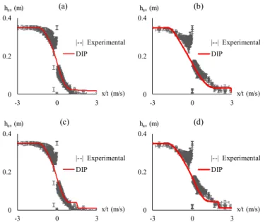
The DIP model and the transient momentum dissipation model are validated against the experiments as follows. The first validation stage consists in running the DIP model using = 0 in equation (1d). The results are shown in Figure 5a-b for Configurations 1 and 2 respectively. The second stage consists in adjusting so as to achieve the best fit between the block-averaged experimental data and the DIP simulation results. The corresponding
0 0.2 0.4 -3 0 3 hav(m) x/t (m/s) Configuration 1 |--| Experimental Refined 2D 0 0.2 0.4 -3 0 3 hav(m) x/t (m/s) Configuration 2 |--| Experimental Refined 2D
simulation results are shown on Figure 5c-d. Introducing a non-zero momentum dissipation coefficient contributes to reduce the shock speed. Bearing in mind the jump relationship for the continuity equation, a slower shock necessarily yields an increased water depth behind the shock. This explains the post-shock water depth in Figures 5c-d compared to Figs. 5a-b.
Fig. 5. Block-averaged, experimental water depths and water depths simulated using the DIP model.
(a) Configuration 1, DIP with = 0. (b) Configuration 2, DIP with = 0. (c) Configuration 1, DIP with = 0.475. (d) Configuration 2, DIP with = 0.4.
Comparing Figures 5a-b and 5c-d shows that the transient momentum dissipation model allows for a better reconstruction of the wave propagation speed of the positive wave. This is particularly visible for Configuration 1, where = 0 clearly yields a strongly overestimated shock speed. Using = 0.475 allows for an improved representation of the shock speed and height in the DIP solution. Similarly, for Configuration 2 (Figs. 5b, d), using = 0 in the DIP model leads to an overestimated shock speed by a factor approximately 3. The best fit with the experimental profile is obtained for = 0.4.
5. Conclusion
The development of accurate flux functions and upscaled momentum source terms remains a key issue to the improvement of porosity-based shallow water models. In the field of urban flood simulation, Riemann IVPs are instrumental to the validation of porosity models in that they allow the wave propagation properties of the solutions to be identified very easily. A salient feature of the urban dam-break problem reported in the present
0 0.2 0.4 -3 0 3 hav(m) x/t (m/s) (a) |--| Experimental DIP 0 0.2 0.4 -3 0 3 hav(m) x/t (m/s) (b) |--| Experimental DIP 0 0.2 0.4 -3 0 3 hav(m) x/t (m/s) (c) |--| Experimental DIP 0 0.2 0.4 -3 0 3 hav(m) x/t (m/s) (d) |--| Experimental DIP
communication is that the pore scale-averaged water depth is shown experimentally to be similar in the (x, t) space. To our best knowledge, experimental evidence for the self-similar behaviour of the solution had never been reported before. Solution self-self-similarity implies that usual, head loss models based on turbulent dissipation (with a head loss proportional to the square of the flow velocity) cannot reproduce the momentum dissipation stemming from the propagation of sharp transients through idealized building layouts. The transient momentum dissipation model proposed in the DIP model, in contrast, allows such self-similarity to be preserved and the accuracy of the solution of the model to be improved. Since the first series of experiments reported in the present paper seem to validate the model, the next issue consists in the parameterization of the momentum dissipation coefficient as a function of the urban geometry and flow variables. Obviously, the experiments reported here will have to be extended to a broader range of configurations in order to provide sufficient information to derive an empirical law for . Given the time-consuming character of urban dam-break experiments, it is expected that a full experimental parameterization of should involve a coupled operation of scale models and numerical simulations.
Acknowledgements
The authors wish to acknowledge the contribution of Fabiola Gangi, Gennaro Pileggi and Samuel Laurent in performing the laboratory experiments. The financial support of Inria-LEMON for researcher mobility funding is gratefully acknowledged.
References
1. A. Defina. Two-dimensional shallow flow equations for partially dry areas. Water Resour. Res. 36, 3251–64 (2000)
2. J.M. Hervouët, R. Samie, B. Moreau Modelling urban areas in dam-break floodwave numerical simulations. In: Proceedings of the international seminar and workshop on rescue actions based on dambreak flow analysis, pp. 1–6 . Seinâjoki, Finland (2000) 3. V. Guinot, S. Soares-Frazão. Flux and source term discretisation in two–dimensional
shallow water models with porosity on unstructured grids. Int. J. Numer. Meth. Fluids
50, 309–345 (2006)
4. S. Soares–Frazão, J. Lhomme, V. Guinot, Y. Zech. Two–dimensional shallow water models with porosity for urban flood modelling. J. Hydraul. Res. 46, 45-64 (2008) 5. B.F. Sanders, J.E. Schubert, H.A. Gallegos. Integral formulation of shallow water
equations with anisotropic porosity for urban flood modelling. J. Hydrol. 362, 19–38 (2008)
6. Schubert, J.E., Sanders, B.F. Building treatments for urban flood inundation models and implications for predictive skill and modeling efficiency. Adv. Water Resour. 41, 49-64 (2012).
7. V. Guinot, B.F. Sanders, J.E. Schubert. Dual integral porosity shallow water model for urban flood modelling. Adv. Water Resour. 103, 16-31 (2017)
8. M. Velickovic. Macroscopic modeling of urban flood with a porosity model. PhD thesis, Université catholique de Louvain, Louvain-la-Neuve (2012)
9. M. Velickovic, S. Soares-Frazão, Y. Zech. Steady-flow experiments in urban areas and anisotropic porosity model. Journal Hydraul. Res. 55, 85-100 (2017)
10. B. Kim, B.F. Sanders, J.S. Famiglietti, V. Guinot. Urban flood modeling with porous shallow-water equations: a case study of model errors in the presence of anisotropic porosity. J. Hydrol. 523, 680–692 (2015)
11. I. Özgen, J. Zhao, D. Liang, R. Hinkelmann. Urban flood modeling using shallow water equations with depth-dependent anisotropic porosity. J. Hydrol. 541, 1165-1184 (2016) 12. V. Guinot. A critical assessment of flux and source term closures in shallow water models with porosity for urban flood simulations. Adv. Water Resour. 109, 133-157 (2017)
13. V. Guinot. Multiple porosity shallow water models for macroscopic modelling of urban floods. Adv. Water Resour. 37, 40–72 (2012)
14. J.A. Cunge, F.M. Holly Jr, A. Verwey. Practical aspects of river computational hydraulics (Pitman Publ., 1980)
15. S. Soares-Frazão, V. Guinot. An eigenvector-based linear reconstruction scheme for the shallow water equations on two-dimensional unstructured meshes. Int. J. Numer. Meth. Fluids 53, 23–55 (2007).