A formal approach to the mapping of tasks on an heterogenous multicore, energy-aware architecture

HAL Id: hal-01412790

https://hal.inria.fr/hal-01412790

Submitted on 8 Dec 2016

HAL is a multi-disciplinary open access

archive for the deposit and dissemination of

sci-entific research documents, whether they are

pub-lished or not. The documents may come from

teaching and research institutions in France or

abroad, or from public or private research centers.

L’archive ouverte pluridisciplinaire HAL, est

destinée au dépôt et à la diffusion de documents

scientifiques de niveau recherche, publiés ou non,

émanant des établissements d’enseignement et de

recherche français ou étrangers, des laboratoires

publics ou privés.

A formal approach to the mapping of tasks on an

heterogenous multicore, energy-aware architecture

Emilien Kofman, Robert de Simone

To cite this version:

Emilien Kofman, Robert de Simone. A formal approach to the mapping of tasks on an heterogenous

multicore, energy-aware architecture. MEMOCODE’16 - 14th ACM-IEEE International Conference

on Formal Methods and Models for System Design, Nov 2016, Kanpur, India. �hal-01412790�

A formal approach to the mapping of tasks on an

heterogenous multicore, energy-aware architecture

Emilien Kofman

Université Côte d’Azur, Inria, CNRS UMR 7248

Robert de Simone

Abstract—The search for optimal mapping of application (tasks) onto processor architecture (resources) is always an acute issue, as new types of heterogeneous multicore architectures are being proposed constantly. The physical allocation and temporal scheduling can be attempted at a number of levels, from abstract mathematical models and operational research solvers, to practical simulation and run-time emulation.

This work belongs to the first category. As often in the embedded domain we take as optimality metrics a combination of power consumption (to be minimized) and performance (to be maintained). One specificity is that we consider a dedicated architecture, namely the big.LITTLE ARM-based platform style that is found in recent Android smartphones. So now tasks can be executed either on fast, energy-costly cores, or slower energy-sober ones. The problem is even more complex since each processor may switch its running frequency, which is a natural trade-off between performance and power consumption. We consider also energy bonus when a full block (big or LITTLE) can be powered down. This dictates in the end a specific set of requirements and constraints, expressed with equations and inequations of a certain size, which must be fed to an appropriate solver (SMT solver in our case). Our original aim was (and still is) to consider whether these techniques would scale up in this case. We conducted experiments on several examples, and we describe more thoroughly a task graph application based on the tiled Cholesky decomposition algorithm, for its relevant size complexity. We comment on our findings and the modeling issues involved.

I. INTRODUCTION

The multiprocessor scheduling problem is a vast and still open topic. Diverse refinements of this problem exist, and most of them are NP-Hard. However the many and recent improvements in SAT and SMT solvers allow to solve medium size instances of such complexity especially since realistic problems rarely reach the worst case complexity. The demand for more computing power in consumer electronics raises again with the new high definition applications. Increasing the frequency in order to run sequential implementations such as video decoding at an acceptable frame rate is no more a valid option. Using parallel implementations and offloading tasks to low-power resources allows to keep our devices warm and smooth. In this work we show a practical approach of multiprocessor scheduling with an SMT solver under realistic hypothesis. This allows us to actually compile and run an application that benefits from this scheduling and check with

This work was partly funded by the French Government (National Research Agency, ANR) through the “Investments for the Future” Program reference #ANR-11-LABX-0031-01.

this implementation whether our modeling assumptions are correct or not.

Not every program is a suitable candidate for this method-ology. Section III motivates the approach and explains the hypothesis that we need to validate. We then explain the energy model that is used in this approach: given a simple CPU energy model, the instant power of a CPU raises linearly with frequency and with the square of the voltage. Even if those non-linearities introduce yet more practical complexity into the already NP-Hard scheduling problem, we are still able to solve non trivial instances, and find sub-optimal but optimized solutions for the most complex instances. Section IV explains how to encode a sequential pseudo code program description and an architecture description to a set of constraints that an SMT solver can handle. Because the result is a simple Gantt timing diagram, we also detail how to transform back this diagram into an executable binary given the technical limitations of the shared memory heterogeneous platform. Section V presents the obtained experimental benefits, the limits of this approach and how to further stretch this limit with better modeling.

We use the running example of a tiled Cholesky algorithm (3x3 to 5x5 tiles) that is built on top of Basic Linear Algebra Subprograms (BLAS). We characterize those Subprograms on each available type of computing resource both in terms of performance and predictability.

II. RELATED WORK

Automatic and assisted parallelization as well as energy optimization are very wide research areas. With the advent of complex computing platforms, carefully modeling the hard-ware is now a mandatory step. Allocating and scheduling a set of jobs on a set of resources can take different forms in the literature, from very theoretical to very applied. However the three steps of ‘characterization, solving, and implementation’ can often be identified.

The current practice in consumer electronic devices in order to save energy is to give the user the ability to setup a “policy” or “governor”. The default policy is often to set every core to the maximum frequency when a new process is submitted to the device (which is the well known “on-demand” power governor). When the program stops all the cores go back to a low performance (and low energy) state. Because consumer electronic devices must support dynamic task appearance, this is a good approach for a best-effort behavior regarding energy

optimization. Embedded signal processing on the contrary often involves a limited set of tasks that must run within a given time budget (such as in a radar processing application), hence the need for static scheduling approaches.

Because every engineer has long been manipulating sequen-tial code in various languages, it is now a difficult problem to extract potential parallelism from this code, and thus previous research has extensively investigated automatic parallelization [15], [2]. Although we give a very naive example of loop nest to graph transformation in order to show the parallelism in the example application, we believe that the reasoning on models in which potential parallelism is less obfuscated (such as graphs and formal models) is also an interesting approach. Pseudo-code or code annotations is also often used for this analysis [4] and can be interpreted as a first step towards formal models.

Reasoning on formal descriptions of the application (and the architecture) allows to guarantee properties on a system, and is an important trend of the current research. The purpose of those formal models is often to ensure properties of the final design such as safety (absence of deadlocks). Because using the model of a Directed Acyclic Graph of task and messages allows to generate the topological sorts (all the valid sequences), the transformations from the studied formal models to this description is often necessary. Synchronous Dataflow graphs [13] and all its variants give a concise description of parallel applications which allow to validate for safety (absence of deadlocks) and is sometimes used as an input model for those scheduling problems [11]. Model-ing hardware features (such as synchronization or message passing) in the same formal description than the application allows to obtain guarantees on the whole system [14], and not only on the application. In recent work, timed events are also considered in order to check throughput properties of cyclic application graphs mapped on multiple resources [17], [18]. Other scheduling techniques include identifying specific task patterns such as fork join, sets of periodic tasks, or pipelines and apply specific heuristics to those patterns [16]. Those heuristics sometimes target specific hardware resource organizations such as network on chips [19], [6].

Finally, another well known set of techniques involves DES (Discrete Event Simulators) and allows to check the result of a scheduling and mapping strategy when studying a scheduling problem. SystemC is an example of DES that has been used that way, including some of its extensions (TLM) that allow to give a coarse description of the hardware and software models when a RTL or functional implementation is not desired. Some tools are built on top of those DES for fast prototyping (Synopsys MCO Platform Architect [9]). Those DES often come with verification tools, which allow the creation of testbenches to check specific cases, sometimes including randomization of the inputs. Those tools thus allow estimation but no optimization [12], [8], unless a model checker is used in place of the DES.

Energy modeling is not often the main purpose of automatic and assisted parallelization [4], [16], [15] although there is a

renewed attention for low-power designs. It requires to add non linear expressions in the model and thus raises greatly the complexity for model checking, although simulation is still an option [9]. Moreover, power modeling involves multiple mechanisms such as frequency scaling and power gating that make both the modeling and the implementation very complex, yet necessary to obtain insightful results [11].

III. THEALGORITHMARCHITECTUREADEQUATION ISSUE

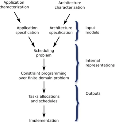
In this section we show the preliminary work of exhibiting the potential parallelism of the input application model with a pseudo-code to DAG transformation. Then, according to the workflow (Figure 1) we encapsulate the results of the characterization experiments into an application model and an architecture model. In this section we describe what we measure, how, and we give evidence that those models are trustworthy. Because a model is always slightly wrong, we quantify the error that they may introduce. Finally, we describe the energy models that allow us to relate the resources speed and their energy consumption.

Scheduling problem

Constraint programming over finite domain problem Application specification Architecture specification Tasks allocations and schedules input models Internal representations Outputs Implementation Application

characterization characterizationArchitecture

Fig. 1: Workflow of our approach

A. Application tasks and task graphs

Various input models would fit our needs, as long as there exist a transformation to a graph-like model with a finite number of task and messages. Synchronous dataflow graphs, with the well known Homogeneous SDF transformations is also an eligible candidate, as well as periodic task systems. We achieve this transformation from a pseudo code description of the tiled Cholesky algorithm such as described in the literature [4], [5].

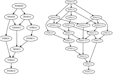
1) Pseudo-code to task graph model: Given a number of tiles T of matrix A we use the tiled Cholesky algorithm (Figure 1) to compute the graph of dependencies between the BLAS level-3 functions (GEMM, TRSM, POTRF and SYRK). We obtain the graphs in Figure 2.

Algorithm 1 Pseudo-code for the tiled Cholesky algorithm Require: number of tiles: T

Require: tiled matrix: A for k=0...T do

A[k][k] = POTRF(A[k][k]) for m=k+1...T do

A[m][k] = TRSM(A[k][k], A[m][k]) end for

for n=k+1...T do

A[i][i] = SYRK(A[n][k], A[n][n]) for m=n+1...T do

A[n][m] = GEMM(A[m][k],A[n][k],A[m][n]) end for

end for end for

Figure 2 shows the data-dependency graph of the tiled Cholesky algorithm for a matrix of 3x3 and 4x4 tiles. We identify separately each function call depending on which tile it reads or writes, hence the numbering in the resulting graph. We add a dependency to the graph for each corresponding read and write. In this model we consider that a task can start only when all its inputs are available.

POTRF00 TRSM20 TRSM10 SYRK10 POTRF11 TRSM21 GEMM12 SYRK20 SYRK21 POTRF22 TRSM(3,1) GEMM(1,2,3) SYRK(3,1) POTRF(2,2) TRSM(3,2) POTRF(1,1) TRSM(2,1) TRSM(3,0) SYRK(3,0) GEMM(0,1,3) GEMM(0,2,3) POTRF(3,3) TRSM(2,0) GEMM(0,1,2) SYRK(2,0) TRSM(1,0) SYRK(1,0) SYRK(2,1) POTRF(0,0) SYRK(3,2)

Fig. 2: Data-dependencies of the tiled Cholesky algorithm for 3x3 and 4x4 tiled matrices (the numbers identify the tile)

B. Architectures, Operating Systems and variability

Multi-programming introduces a lot of variability in the execution of data-independent jobs, due for instance to pre-emption and interrupts. Using a standard environment also comes with some benefits and tools that we can use to check how much variability multi-programming introduces, and even try to avoid it. For instance we expect that thread pinning

(force a thread to run and stay on a specific core) will reduce this variability. In this section we describe why variability can be introduced in this setup, and how to keep it low.

WCET (Worst Case Estimation Time) is a difficult topic that we don’t fully tackle here. We address the case where the tasks costs do not have much variability which we carefully check in section III-C. We consider the case of an embedded system, where the resources are not shared to multiple users. In that case the variability is mainly due to different behaviors of the tasks depending on their input data. The most flagrant example of “data-dependent” tasks are the sparse matrix operation algorithms, where their dense counterpart are however “data-independent”. For instance we expect a matrix multiplication routine to execute the same number of instructions for fixed matrix sizes whatever values contained in those matrices. This hypothesis does not hold in the case of a sparse matrix multiplication algorithm, because then the algorithm behaves differently depending on the sparsity of the matrices. In that case we could also over-approximate the cost of the matrix multiplication task, which is why the WCET metric is sometimes used. An important part of the characterization step consists in determining the Average Case Estimation Time (ACET), and verifying that its standard deviation has a reasonable value. This reasoning does not apply in the case of an already parallel implementation of a matrix multiplication algorithm, or would require some implementation effort in order to be predictable (which is also what we try to achieve with this methodology).

Our experimental setup allows us to control thread pinning and core frequencies. Because the scheduler of the operating system may decide to switch context or preempt our tasks, we also use a high scheduling priority to further reduce the variability of the task costs. We used the OpenBLAS kernels (implementations of the BLAS level 3 kernels) and carefully check that they run as single threaded kernels, since we aim at building a multithreaded application on top of them. As expected, their multithreaded implementations are much less predictable, with according to our measurements one order of magnitude difference in variability of number of cycles for the matrix multiplication multithreaded implementation without task pinning. This approach distinguishes every sub-program as a sequential execution such that the application that uses it can be both parallel and predictable. A distributed memory architecture such as scratch-pad memories would certainly allow much more predictability, since the implementation would be allowed to control the message passing as well, but because it is not a widespread architecture and because we need also energy saving mechanisms we study this problem on a shared memory architecture, and we try to limit the memory conflicts. The example architecture is a big.LITTLE ARM implementation with frequency scaling illustrated Figure 3. The experiments of sections III-C are conducted with the same experimental setup than the one described in section V-A.

A15

A7

A15

A7

Fig. 3: bigLITTLE ARM architecture

C. Variability of ground level tasks

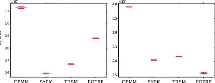
We estimate the cost of the task with their number of cycles when executed on the target Odroid-XU3 system. In this section we examine and challenge the low-variability hypothesis. Figure 4 shows the number of cycles when a single threaded BLAS (from the openBLAS benchmark) is executed on the target, along with the Violin error plot and the extreme values. We observe a very stable execution for each of the BLAS we use. We use the coefficient of variation as the variability metric (standard deviation over mean), the results are presented Table I and Figure 4. We perform those measurements by reading the hardware counters through the “perf_events” Linux kernel interface [7]. We use the costs defined in Table I in the next sections in order to obtain parallel schedules for this heterogeneous architecture. In this experiment, the costs of the BLAS kernels are in the same order of magnitude. When the problem combines very small costs with very large costs, the approach may require either to omit the small tasks or to merge them such that the costs of the jobs remain in the same order of magnitudes.

0.6 0.7 0.8 0.9 1.0 1.1 ×107 1.5 2.0 2.5 3.0 3.5 4.0×10 7 Cycles

GEMM SYRK TRSM POTRF GEMM SYRK TRSM POTRF

Fig. 4: Predictability of BLAS lvl3 kernels on A7 and A15 architectures (in number of cycles), for 200x200 samples tiles

D. Energy vs performance modeling

This section details the energy saving mechanisms and validates their use with this model. Then we show how

TABLE I: Costs of the BLAS kernels (106 cycles)

GEMM SYRK TRSM POTRF

A15 mean 11 6 7 9

cv (%) 0.29 0.21 0.19 0.08

A7 mean 39 20 21 16

cv (%) 0.11 0.23 0.11 0.64

we found realistic values for Cr and activity factor on the

big.LITTLE Exynos5422 target.

1) Dynamic Voltage and Frequency Scaling: Given the Operating Point (OPP) o = (V, f ) of a resource r, we know from previous work [3] that we can model its instant power with the following:

P (r, o) = Cr· V2· f · A (1)

We define the variables of Equation 1 and we give their dimension:

• Cr[Farads]: the model capacitance of the CPU (roughly

proportional to the number of the switching devices, i.e. the number of transistors)

• V [Volts]: the voltage of the current operating point • f [Hertz]: the frequency of the current operating point • A [dimensionless]: An activity factor that models the

average number of bit flips that the task will cause on the resource. Although it is specific to each pair of task and resource and often approximated to 1.

Then for a task t running on the resource r at OPP o, given that the task costs Cycycles when running on this resource, the

task will last Cy

fo, thus we can model the consumed energy with

the expression 2. We observe in this expression that E(t) does not depend on fo, but only on Vo (which usually raises with

fo). This means that running a task at a low frequency actually

consumes less energy than running it at high frequency, even though it lasts longer. This is the purpose of frequency scaling. Power models sometimes include static power consumptions, which is the amount of power that leaks through the gates as long as the chip is powered. This means that running a task at a very low frequency could actually consume more energy because of static power. Given the measured power levels of Figure 5 we do not consider static power in our approach.

E(t) = Cy fo

· P (r, o) = Cr· Cy· Vo2· A (2)

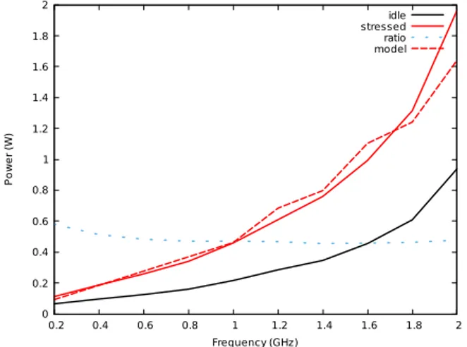
Figure 5 shows the instant power of the A15 Big resource when it is computing. We used the stress task (from the linux utility “stress”, which simply does square root computations) to apply a computation intensive workload. Because for each OPP we know the frequency and the voltage (we set it), and the power sensor allows to sample the instant power, we are able to find realistic values for the capacitance of A7 and A15 cores (resp. 500pF and 100pF). We also sample the instant power when the resource is idle, depending on its running frequency which suggests that the activity factor of the idle state Aidleis Aactive/2. We consider Aactive= 1 even though

this activity factor actually depends on the task which runs and thus might vary depending on the BLAS kernel. We observed small but non negligible variations depending on the task, but the very limited power sensor sampling rate and resolution does not allow to conduct a full characterization. With a proper electronic setting, this value could be integrated into our models with no additional complexity regarding the scheduling problem. 0 0.2 0.4 0.6 0.8 1 1.2 1.4 1.6 1.8 2 0.2 0.4 0.6 0.8 1 1.2 1.4 1.6 1.8 2 P o w e r (W ) Frequency (GHz) idle stressed ratio model

Fig. 5: Instant powers of the tasks vs frequency

2) Power gating: We consider the static power of the resources but we do not consider that the resources are able to turn on and off during a run. If at least one task has to execute on one resource, then this resource is always on in the steady state system. Then it will be idle in its spare time, at its lowest power OPP but it will still consume power. Thus it is interesting to know if a scheduling problem can be solved by powering ON only a subset of the resources in a machine. The instant power of the system depends on time because the resources are allowed to change their operating point in time. Given the instant power P (R), the energy with a dimension of W atts · seconds = J oules is thus calculated for each resource r over the duration of the schedule (which means from zero to makespan M ).

Ea(r) = Z t=M t=0 P (r) dt (3) = Cr· Z t=M t=0 V2· f · A dt (4)

Let tobe the opp for task t, this means that each resources

r running at opp o consumes:

E(r, o) = Cr· X t∈T asks|to=o ·Cy f · V 2 o · f E(r, o) = Cr· X t∈T asks|to=o Cy· Vo2

Let Orbe the set of OPPs of resource r, the energy consumed

by the tasks running on r is:

Ea(r) =

X

o∈Or

E(r, o)

We call that quantity “active” energy consumption.

Finally let Pidle be the idle instant power of the resource,

tpt the physical time duration of task t and tmap the resource

where t is mapped. The idle energy can also be expressed as a discrete sum:

Ei(r) = Pidle· (M −

X

t∈T asks|tmap=r

tpt) (5)

Thus, the consumed energy of the system is:

E = sum(Ei(r) + Ea(r) | r ∈ R) (6)

That E is what we try to minimize. Figure 13 gives a simple example where the consumed energy can be optimized without performance penalty.

3) Motivating example: Lowering the frequency of a task does not always mean that the optimization criteria is de-graded. For instance if we want to optimize makespan, we can find very simple application descriptions of tasks and depen-dencies which give evidences that energy can be optimized with a preserved makespan. Figure 6 is a typical problem instance with a split/join of unbalanced tasks, where slack time can be used to save energy. Generally speaking, this applies to each non critical path. This also gives evidence that the solver will be able to optimize energy if we allow more slack time from the optimal makespan schedule.

CPU1 CPU0 0 0.5 1 1.5 2 2.5 3 3.5 4 A B sp lit jo in time (ms) CPU1 CPU0 0 0.5 1 1.5 2 2.5 3 3.5 4 jo in B A sp lit time (ms)

Fig. 6: Non energy optimized vs optimized split join pattern (red tasks run with high instant power)

When the application graph is not a simple unbalanced two workers split/join, it is (computationally speaking) much harder to decide the allocation and the operating point in order to obtain an optimized schedule. For a few tasks with precedences it might even be hard for a human to optimize for makespan, considering only high frequency operating points. Then, the more slack time, the higher possible energy optimization, and the larger state space to explore. Thereafter we explain how to encode those problems into a solver in order to address them automatically. Then we use this constraint programming encoding to schedule the tiles of the tiled matrix Cholesky factorization running on an heterogeneous multicore.

IV. ENCODING INTOCONSTRAINTS OVER FINITE DOMAINS

The metrics that we use to characterize the tasks and the platform actually belong to discrete sets even when some mathematical property is used to define a new variable. For instance the time that a task will last depends on the resource that runs it, and the frequency at which the task runs. This means that the task duration variable is within the set of resources × OPPs. The problem is thus defined as a Constraint Logic Programming over finite domains CLP(fd).

A. Linear Programming

Since the problem mostly includes inequalities and linear equalities such as tstop = tstart + tduration, it is a natural

idea to model it using linear programming. In heterogeneous scheduling problems, tdurationdepends on tmap, and if

mul-tiple operating points exist, it also depends on topp: we need

to introduce a zero-one “decision variable” in both cases. It is easy to encode such constraints using an if-then-else construct, which does not exist in LP most solvers. Another example is the “exclusive OR” constraints of non-overlapping two tasks that use the same resource (see Section IV-C). Some tricks exist but require to introduce artificial variables and quantities that must be chosen carefully. Recent solvers (such as CPLEX) introduce specific constructs that translate to other theories (such as Mixed Integer Programming). Because combining theories is the purpose of “SAT Modulo Theories” solvers, we try to use an SMT solver instead.

B. Costs to finite sets

Let us define the simplest version of the heterogeneous scheduling problem, which is a set of tasks T and a set of resources R. Each resource is associated with a micro-architecture µ ∈ A. The cost of a task in number of cycles is associated to a microarchitecture Cy(t, µ) which is an input of the problem. This means that we can enumerate the possible task costs by iterating the combinations in T × A. Given the obtained Average Case Execution Time estimations of the costs and given the admissible frequencies, the elements of those new set are rationals. Because not every solver have support for the rational type (for instance the SMTLib language [1] does not define the rational type), we explain how to reduce the set to a set of integers.

For example, given the objective of makespan optimization for the three tasks A,B,C of cost 4MCy, 2MCy, 3MCy on two homogeneous cores (C0 and C1) with different speed 1GHz and 2Ghz: we can bound the problem in time by evaluating one possible schedule, for instance the slowest schedule of 9ms. Then, we know that A is either 4 or 2ms, B: 1 or 2, C: 1.5 or 3. Because we are interested in the solutions where the tasks starts and stops are “aligned”, a 1/2 ms which is the Greatest Common Divisor looks like as a very suitable time step. We generalize this by collecting the possible durations of timed events, finding their common divisor and using it as a time step. By construction, this allows to transform every physical time duration into an integer, as well as the time bound. This allows to transform our problem to an Integer Programming

problem. Because there exists a finite set of admissible instant powers, the same is conducted for the energy model.

C. Constraints

In this section we list the constraints that we use in order to generate the schedules. Let T be the set of tasks, let R be the set of resources and O be the set of operating points, tmap∈ R

and topp∈ O. Let M be the set of messages (or precedences),

with sender and receiver two functions from M to T . The integer table costs is calculated according to the previous sections. A timebudget is specified, and the makespan is a variable of the problem that may be optimized. Let rip be

the idle power of the resource r, and op the instant power of

opp o. We first define application and allocation scheduling constraints (Algorithm 2), and if the problem requires the power model we add the constraints defined in Algorithm 3.

Algorithm 2 Constraints

Require: costs table: T × R × O Require: timebudget

for t ∈ T do

tstart, tstop, tduration∈ N

tstop= tstart+ tduration

tstop≤ makespan

makespan ≤ timebudget tduration= costs[t][tmap][topp]

end for

for (v, u) ∈ T2_{| v! = u do}

umap== vmap =⇒ ustart≥ vstop⊕ ustop≥ vstart

end for for m ∈ M do

receiver(m)start≥ sender(m)stop

end for

Algorithm 3 Energy related variables and constraints for o ∈ O do

ouptime=Pt∈T(tduration| tmap== r, topp== o)

oenergy= op∗ ouptime

end for for r ∈ R do

ruptime=Po∈O(ouptime)

rdowntime= makespan − ruptime

if ruptime == 0 then

renergy = 0

else

renergy =P_o∈O(oenergy) + rip× rdowntime

end if end for

D. Back from model to code

Our optimized versions of the tiled Cholesky algorithm use many tools and libraries in order to better control the platform. For the BLAS kernel implementations, the Gnu Scientific Library with OpenBLAS linking was used. libcpufreq allows

to change the frequency of a core, libpthread allows to fork and join threads, as well as pinning them to specific cores with the functions defined in sched.h. The result of the SMT solver allows us to build a schedule for each resource, including the data dependencies across resources that we transform to syn-chronization (because the memory is shared). The functional aspect of the code is tested with assertions that can be removed by the preprocessor with proper symbol definition.

1) Minimal energy schedules: Since the A7 little core can run at the lowest instant power available on the platform, the schedule that minimizes energy is the one that uses only the A7 little core, whatever the resulting makespan. For instance for a 3x3 tiled Cholesky algorithm with minimized energy consumption we obtain the schedule of Figure 7 which is simply one of the many valid topological ordering of the graph presented in Figure 2

POTRF(0,0)->TRSM(1,0)->SYRK(1,0)-> TRSM(2,0)->POTRF(1,1)->GEMM(0,1,2)->

TRSM(2,1)->SYRK(2,0)->SYRK(2,1)->POTRF(2,2)

Fig. 7: Topological order of the 3x3 tiled Cholesky task graph

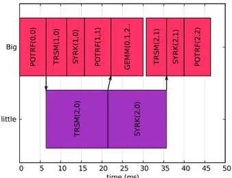
2) Minimal makespan schedules: We now study the sched-ule obtained when minimizing makespan. Its transformation to a shared memory multithreading environment allows to transform the messages into synchronizations. The highest frequencies (hence the fastest but also the highest instant powers) are selected in order to minimize the makespan, but there is no straightforward solution. The solver outputs a solu-tion (schedule in Figure 8) from which we generate the code skeleton to implement it in the shared memory environment. The messages (arrows in Figure 9) are transformed to POSIX semaphores. little Big 0 5 10 15 20 25 30 35 40 45 50 S Y R K (2 ,1 ) G E M M (0 ,1 ,2 .. P O T R F( 1 ,1 ) P O T R F( 2 ,2 ) S Y R K (1 ,0 ) S Y R K (2 ,0 ) T R S M (2 ,1 ) T R S M (2 ,0 ) T R S M (1 ,0 ) P O T R F( 0 ,0 ) time (ms)

Fig. 8: Makespan optimal schedule for 3x3 tiled Cholesky algorithm on a 1+1 bigLITTLE architecture (red means high instant power)

3) Multiobjective optimization schedules: Finally, the schedules obtained when minimizing energy and bounding

Thread #0 pin to big core

set frequency start Thread #1 POTRF(0,0) WRITE(0) TRSM(1,0) SYRK(1,0) READ(2) GEMM(0,1,2) POTRF(1,1) TRSM(2,1) READ(1) SYRK(2,1) POTRF(2,2) Thread #1

pin to LITTLE core set frequency READ(0) TRSM(2,0) WRITE(2) SYRK(2,0) WRITE(1)

Fig. 9: 3x3 Makespan optimal multithreaded pseudo code

makespan may contain both synchronizations and frequency changes. We implement the frequency changes with the cpufreq library. This library is the one that implements the energy governors in the linux kernel, and allows to set the governor for each core (userspace, powersave, conservative, ondemand, performance, ...). The typical setup uses either powersave/ondemand/performance. The userspace behavior as its name suggests allows to change the current frequency from a userspace program.

V. RESULTS

In this last section we give the obtained schedules and objective values for different optimization requests and we show how much energy savings one could expect when giving the makespan a bit of slack compared to its optimal value obtained in the previous experiments. Finally, we translate the schedules to executable parallel implementations. Then, we run the obtained binaries on the Exynos5422 platform and we try to evaluate how faithful is the generated implementation.

A. Experimental setup

We run all the experiments on an embedded development board (Odroid XU3) featuring a Samsung Exynos5422 ARM bigLITTLE processor of four A7 cores and four A15 cores such as the one described in Figure 3. The bigLITTLE technology is an heterogeneous MP-SoC architecture designed by ARM. Samsung implemented it in the Exynos5422 Chip, which was used by the Corean company “Hardkernel” to build the Odroid board. The platform runs a Linux Ubuntu 15.10 operating system with a 3.10 kernel that was patched in order to enable hardware cycle counters. In the experiments described in section V we sometimes consider 1,2 or 4 cores of each (big and LITTLE). The platform is equipped with instant power sensors that allow us to sample instant power of each cluster (of big or LITTLE cores) and a performance monitoring unit (PMU) that allows to access relevant metrics such as cycle counts through the perf Linux API [7].

TABLE II: Results obtained with the modeling and solving (time in milliseconds)

3x3 4x4 5x5

N.of tasks (and messages) 10 (12) 20 (30) 35 (60)

Optimal makespan 46 39 ≤ 38

Sequential makespan 55 51 49

ASAP makespan 55 45 44

Energy optimal makespan 350 349 343

B. Makespan optimization

As expected when the number of tiles grows, the number of tasks and task dependencies also grows. The overall number of samples is constant, thus the number of samples per tile de-creases when the number of tiles inde-creases. The costs obtained in Table I have been updated with the corresponding values for the tiles of different sizes corresponding to our experiments. We were able to solve the non trivial examples of 3x3 and 4x4 tiled Cholesky algorithm running on two heterogeneous cores optimally, and we got a sub-optimal (but still optimized) result for the 5x5 tiled Cholesky algorithm. Because the solver is very efficient at finding satisfiable solutions when there is a lot of slack time [10], even with a much larger number of tasks and messages (resp. 35 tasks and 60 messages in the 5x5 example), it is able to find a solution, and to get an optimal or optimized solution. We experiment different problems with higher theoretical complexity and we report their practical complexity in section V-D.

Because the solver approach also allows to implement heuristics by doing successive calls to the solver and changing the objective function, we can compare the obtained schedules to one of the greedy “As Soon As Possible” (ASAP) sched-ules. In order to obtain this schedule we sort the tasks by topological order and we add them in this order to the set of constraints, asking for makespan minimization: the strategy becomes greedy, hence sub-optimal but allows as expected to obtain schedules for large instances. We also compare our results to the naive sequential implementation with all tasks running on the fastest resource, at the highest frequency. In either case we obtained significant improvement. For the 5x5 tiled Cholesky algorithm graph, we obtained an optimized but sub-optimal result, still better than naive and ASAP implementations. The results also suggest that the divide and conquer strategy actually works, since the makespan decreases when the number of tiles increases (for the same matrix size). The exhaustive results are presented in Table II.

The synthesized implementation is compared to those pre-dicted values and its predictability is evaluated with the same coefficient of variation used in section III. The results are presented in Table III. Of course running those programs requires a high level of privileges since it requires access to critical hardware features, such as modifying frequencies. This is acceptable on an embedded system since there is probably only one user (sometimes there is even no operating system) but it is probably not acceptable on a shared server with no

proper isolation. When the tiles are too large, input data of the BLAS kernels do not fit in the data caches. This can increase variability and lower performance, as the result for the 3x3 case suggests. Adapting tile sizes to cache size such that the generated schedule restricts as much as possible the access to shared levels of the memory would be an interesting addition. The 4x4 and 5x5 results do not suffer from this issue because they compute on smaller tiles. The results in those latter cases are very close to the predicted results, which suggests a very faithful model.

TABLE III: Execution time and variability of the generated implementations

3x3 4x4 5x5 Time (ms) 53.2 40.5 39.6 cv (%) 0.89 0.53 0.77

C. Energy optimization

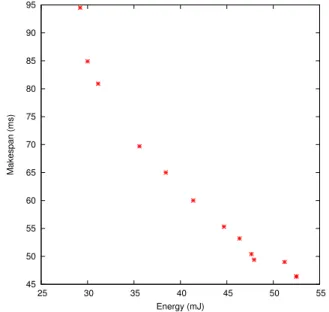
As well as for makespan optimization, the obtained makespans when optimizing for energy are very close to the predicted values (for instance the implementation of Figure 11 lasts 76ms). We now generated Pareto fronts for those models and examine the corresponding implementations. Figure 10 shows a subset of the schedules that are on the Pareto front for the 3x3 algorithm. The power sensor that was used in the section III-D in an on-board device that is connected to the big.LITTLE through an I2C Bus. It is not very precise and allows sampling at a slow rate (not at the 1kHz rate that we would need). However, we can at least check the instant power when running different implementations, and the very precise timings allow to calculate the consumed energy.

45 50 55 60 65 70 75 80 85 90 95 25 30 35 40 45 50 55 Makespan (ms) Energy (mJ)

Fig. 10: Pareto front for the 3x3 algorithm

The fastest theoretical schedules for 3 and 4 tiles report a 52.5mJ and 45.1mJ energy consumption. The instant power is

sampled when the implementations run and we obtain 1.24W and 1.27W, which corresponds (according to the obtained exe-cution times of Table III) to energy consumption of 66mJ and 51mJ. We do the same for the schedules where the time budget is twice the optimal makespan (Figure 11), those schedules report (resp.) and 30.0 and 30.5mJ, and the implementations report 45.4 mJ and 46.3 mJ. Although the model is not correct, we obtained valid implementations within a given time budget, with a significant energy optimization.

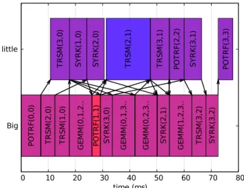
Big little 0 10 20 30 40 50 60 70 80 S Y R K (1 ,0 ) T R S M (3 ,2 ) P O T R F( 0 ,0 ) T R S M (3 ,1 ) G E M M (1 ,2 ,3 .. S Y R K (3 ,0 ) P O T R F( 3 ,3 ) P O T R F( 2 ,2 ) S Y R K (3 ,1 ) S Y R K (2 ,0 ) T R S M (2 ,1 ) T R S M (3 ,0 ) T R S M (2 ,0 ) T R S M (1 ,0 ) G E M M (0 ,2 ,3 .. S Y R K (2 ,1 ) P O T R F( 1 ,1 ) G E M M (0 ,1 ,2 .. S Y R K (3 ,2 ) G E M M (0 ,1 ,3 .. time (ms)

Fig. 11: 4x4 tiled Cholesky schedule optimized (sub-optimal) for energy, with a time budget of twice the optimal

D. Further scalability results

There are a number of direct extensions one can apply to the previous modeling and encoding effort, with in mind the idea of checking how the method can be pushed to its limits in terms of complexity regarding solver efficiency. Already the parametric aspect of Cholesky algorithm allows to scale up a range of applications. Modeling the multiplicity of process frequencies, or multiple cores in each compute block also increases the demand on solvers. We experiment with such extensions now, looking for limitations as they occur. As the Figure 3 suggests, our experimental setup allows to run up to 4 big and 4 little cores. In the previous experiments we have been using only 1+1 cores. We synthesize the results related to scalability in Table III.

TABLE IV: Solver time vs number of cores and number of tiles #cores (big+LITTLE) 1+1 2+2 4+4 #tiles 3x3 2s 2s 3s 4x4 1min48s 8s 11s 5x5 >1h 10s 28s

From the numbers of Table III it appears that, although the scheduling complexity is on the whole related to the size of the problem (the system of constraints to solve), this connection is not as regular as it may seem, and the impact of whether regular or irregular solutions emerge can dominate the size complexity. So certainly much more remains to be done on predicting when (and how) relative dimensioning may favor regularity, and so solver efficiency, in the universe of solutions. Moreover, although in the makespan optimization problem the highest frequencies alone can achieve the optimal results, some of the optimal results can include low frequency tasks (as figure 13 suggests). We observed for instance an impact of the number of operating points on the solver time in the “4 tiles running on 2 little and 2 big cores” problem. 6x6 tiled problems timed out after one hour. The irregularities in the scalability suggest that the constraint programming models can be further improved.

E. Improved modeling for scalability

In the case of the Cholesky matrix factorization, the task graph is not a simple structure. Other applications include more structured patterns such as “split/join” graphs. For in-stance radars perform multidimensional Fast Fourier Trans-forms to identify shapes. We experimented with the 2D radar application described in Figure 12. The former approach would consist in instantiating one FFT occurrence for each worker of both “split/join”. Another approach consists in instantiating one tasks for each resource, and allow them to have a variable duration as long as their sum complete the total work. The whole problem must also include relevant constraints from Algorithm 2. In that case of an heterogeneous architecture, the latter approach also allows a better load balancing.

Input Capture FFT0 FFTi FFTn Image Transpose FFT0 Detection FFTi FFTn

...

...

Fig. 12: 2D radar application

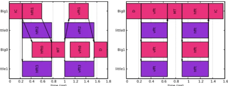
In the case of four resources (two big and two little cores), the solver returns the optimal solution for up to 6 tasks (n = 6 on Figure 12)for each split/join in a matter of seconds. More complex instances of this naive mode (n > 6) timed out at 10 minutes of search. In this case the naive approach does not

scale enough to operate on an image (where usually n > 210_).

By defining only two tasks of variable duration, we are able to balance the work of the split/join patterns.

little1 Big0 little0 Big1 0 0.2 0.4 0.6 0.8 1 1.2 1.4 1.6 1.8 IC _hfft1 v ff t2 h ff t0 h ff t3 v ff t1 D h ff t2 v ff t3 M T v ff t0 time (ms) little1 Big1 little0 Big0 0 0.2 0.4 0.6 0.8 1 1.2 1.4 1.6 v ff t D h ff t v ff t h ff t h ff t IC h ff t v ff t v ff t M T time (ms)

Fig. 13: Results for the former (4 tasks for each split join) and latter approach on the radar application

VI. CONCLUSION

Because shared memory architectures do not allow explicit message passing, the cost of moving data from memory to the L1 caches is not explicitely studied here, it is included in the characterization step of Section III. The constraint pro-gramming approach provides a composable environment, thus including message costs for a distributed memory accelerator would be a feasible and interesting addition. It would also be easier to characterize and control the variability in such case. Unfortunately, distributed memory embedded systems such as scratchpad architectures are not widespread.

We do not address the temperature issue in this work. Adding a temperature model would probably require reason-ing over a much larger timescale. However, because power consumption raises with temperature this might be an inter-esting and tricky addition. Future work also includes other model refinement such as introducing other timed events (or penalties) in order to have better modeling which might be necessary for smaller datasets. It is worth noting that refining the models does not always mean that the state space will be larger, for instance introducing a penalty for frequency change actually reduces the state space.

Static scheduling is applicable to other signal or image pro-cessing application that admit a divide and conquer algorithm, assuming the ground level tasks are not data-dependent. It is for instance applicable to the Fast Fourier Transform which can be divided into smaller Fast Fourier Transforms, as well as LU and QR matrix factorization and generally speaking any application built on top of the BLAS kernels. In this paper we show with a realistic running example how to use a SMT solver for static scheduling, how to model energy aware architectures and how to trade time for energy with this modeling technique. We investigated the scalability of this approach and applied the same workflow to other examples, including synthetic and realistic applications (FFT, Platooning application). Our results also show that solving realistic struc-tured problems may require more modeling effort. Producing optimized and energy efficient code is a great challenge for the new upcoming battery powered devices.

REFERENCES

[1] C. Barrett, P. Fontaine, and C. Tinelli. The smt-lib standard version 2.6. 2010.

[2] C. Bastoul, A. Cohen, S. Girbal, S. Sharma, and O. Temam. Putting polyhedral loop transformations to work. In Languages and Compilers for Parallel Computing, pages 209–225. Springer, 2003.

[3] P. Bose, M. Martonosi, and D. Brooks. Modeling and analyzing cpu power and performance: Metrics, methods, and abstractions. Tutorial, ACM SIGMETRICS, 2001.

[4] G. Bosilca, A. Bouteiller, A. Danalis, T. Herault, P. Lemarinier, and J. Dongarra. Dague: A generic distributed dag engine for high perfor-mance computing. Parallel Computing, 38(1):37–51, 2012.

[5] A. Buttari, J. Langou, J. Kurzak, and J. Dongarra. A class of parallel tiled linear algebra algorithms for multicore architectures. Parallel Computing, 35(1):38–53, 2009.

[6] B. D. de Dinechin, P. G. de Massas, G. Lager, C. Léger, B. Orgogozo, J. Reybert, and T. Strudel. A distributed run-time environment for the kalray mppa®-256 integrated manycore processor. Procedia Computer Science, 18:1654–1663, 2013.

[7] A. C. de Melo. The new linux’perf’tools. In Slides from Linux Kongress, 2010.

[8] N. Dhanwada, I.-C. Lin, and V. Narayanan. A power estimation methodology for systemc transaction level models. In Proceedings of the 3rd IEEE/ACM/IFIP international conference on Hardware/software codesign and system synthesis, pages 142–147. ACM, 2005.

[9] B. Fischer, C. Cech, and H. Muhr. Power modeling and analysis in early design phases. In Proceedings of the conference on Design, Au-tomation & Test in Europe, page 197. European Design and AuAu-tomation Association, 2014.

[10] R. Gorcitz, E. Kofman, T. Carle, D. Potop-Butucaru, and R. De Simone. On the scalability of constraint solving for static/off-line real-time scheduling. In Formal Modeling and Analysis of Timed Systems, pages 108–123. Springer, 2015.

[11] S. Holmbacka, E. Nogues, M. Pelcat, S. Lafond, and J. Lilius. Energy efficiency and performance management of parallel dataflow applica-tions. In Design and Architectures for Signal and Image Processing (DASIP), 2014 Conference on, pages 1–8. IEEE, 2014.

[12] H. Lebreton and P. Vivet. Power modeling in systemc at transaction level, application to a dvfs architecture. In Symposium on VLSI, 2008. ISVLSI’08. IEEE Computer Society Annual, pages 463–466. IEEE, 2008. [13] E. A. Lee and D. G. Messerschmitt. Synchronous data flow. Proceedings

of the IEEE, 75(9):1235–1245, 1987.

[14] J.-V. Millo, E. Kofman, and R. D. Simone. Modeling and analyzing dataflow applications on noc-based many-core architectures. ACM Transactions on Embedded Computing Systems (TECS), 14(3):46, 2015. [15] S. Pop, A. Cohen, C. Bastoul, S. Girbal, G.-A. Silber, and N. Vasilache. Graphite: Polyhedral analyses and optimizations for gcc. In Proceedings of the 2006 GCC Developers Summit, page 2006. Citeseer, 2006. [16] Y. Sorel. Syndex: System-level cad software for optimizing distributed

real-time embedded systems. Journal ERCIM News, 59(68-69):31, 2004. [17] S. Stuijk. Predictable mapping of streaming applications on

multipro-cessors, 2007.

[18] S. Stuijk, M. Geilen, and T. Basten. Sdfˆ 3: Sdf for free. In null, pages 276–278. IEEE, 2006.

[19] W. Thies, M. Karczmarek, and S. Amarasinghe. Streamit: A language for streaming applications. In Compiler Construction, pages 179–196. Springer, 2002.