Household Labour Supply and the Marriage Market in the UK, 1991-2008

(1)

HAL Id: halshs-01476509

https://halshs.archives-ouvertes.fr/halshs-01476509

Submitted on 3 Jun 2017

HAL is a multi-disciplinary open access archive for the deposit and dissemination of sci-entific research documents, whether they are pub-lished or not. The documents may come from teaching and research institutions in France or abroad, or from public or private research centers.

L’archive ouverte pluridisciplinaire HAL, est destinée au dépôt et à la diffusion de documents scientifiques de niveau recherche, publiés ou non, émanant des établissements d’enseignement et de recherche français ou étrangers, des laboratoires publics ou privés.

Household Labour Supply and the Marriage Market in

the UK, 1991-2008

Marion Goussé, Nicolas Jacquemet, Jean-Marc Robin

To cite this version:

Marion Goussé, Nicolas Jacquemet, Jean-Marc Robin. Household Labour Supply and the Mar-riage Market in the UK, 1991-2008 . Labour Economics, Elsevier, 2017, 46, pp.131-149. �10.1016/j.labeco.2017.02.005�. �halshs-01476509�

(2)

See discussions, stats, and author profiles for this publication at: https://www.researchgate.net/publication/313619294

Household Labour Supply and the Marriage

Market in the UK, 1991-2008

Article in Labour Economics · January 2017 CITATIONS

0

READS

10

3 authors, including: Some of the authors of this publication are also working on these related projects: Science popularization

View project truth telling under oath

View project Nicolas Jacquemet Ecole d'économie de Paris 62 PUBLICATIONS 246 CITATIONS SEE PROFILE

(3)

Household Labour Supply and the Marriage Market

in the UK, 1991-2008

⇤

Marion Goussé† _{Nicolas Jacquemet}‡ _{Jean-Marc Robin}§

January 2017

Abstract

We document changes in labour supply, wage and education by gender and marital status using the British Household Panel Survey, 1991-2008, and seek to disentangle the main channels behind these changes. To this end, we use a version of Goussé, Jacquemet, and Robin (2016)’s search-matching model of the marriage market with labour supply, which does not use information on home production time inputs. We derive conditions under which the model is identified. We estimate diﬀerent parameters for each year. This allows us to quantify how much of the changes in labour supply, wage and education by gender and marital status depends on changes in the preferences for leisure of men and women and how much depends on changes in homophily.

Keywords: Search-matching, sorting, assortative matching, collective labour supply, structural estimation.

JEL classification: C78, D83, J12, J22.

⇤_{This paper is a revised and augmented version of CeMMAP Working Paper n}o_{07-13, entitled “Assortative}

Matching and Search with Labor Supply and Home Production, which Jean-Marc Robin presented during the Adam Smith lecture in the joint EALE/SOLE congress in Montreal in May 2015. We gratefully acknowledge financial support from ANR-GINDHILA. Jacquemet acknowledges financial support from the Institut

Universi-taire de Franceas well as ANR-10-LABX-93-01. Part of this work has been completed while he was at Université

de Lorraine (BETA). Robin acknowledges financial support from the Economic and Social Research Council through the ESRC Centre for Microdata Methods and Practice grant RES-589-28-0001, and from the European Research Council (ERC) grant ERC-2010-AdG-269693-WASP.

†_{Université Laval; kmailto:marion.gousse@ecn.ulaval.ca; BDepartment of Economics, Pavillon De Sève,}

G1V0A6 Québec (QC), Canada.

‡_{Paris School of Economics and University Paris 1 Panthéon-Sorbonne; knicolas.jacquemet@univ-paris1.fr;}

BCentre d’Economie de la Sorbonne, MSE, 106 Bd. de l’hôpital, 75013 Paris, France.

§_{Sciences Po, Paris and University College of London; kjeanmarc.robin@sciences-po.fr; BSciences-Po,}

(4)

1 Introduction

One of the key issues in understanding how tax policies aﬀect labour supply is the intra-household allocation of time and consumption. This is in particular the case of welfare benefits, such as the Working Family Tax Credit program in the UK and the Earned Income Tax Credit in the US, aimed at providing work incentives and a safety net against poverty at the same time. The models used to address these issues typically take the household as a unit with unitary preferences (from Eissa and Hoynes, 2004, to the recent work of Blundell, Dias, Meghir, and Shaw, 2016), and while the collective models of the family (Chiappori, 1988, 1992) oﬀer a solution for improvement by modeling intra-household resource allocation, the interest of this framework for policy evaluation is hampered by its inability to predict the impact of welfare policies on the sharing rule.1 _{The evaluation of welfare policies for the family thus ultimately requires an} equilibrium model of match formation and intra-household resource allocation.

Goussé, Jacquemet, and Robin (2016), hereafter GJR, develop a search-matching and bar-gaining model of the marriage market, à la Shimer and Smith (2000), in which they add labour supply and household production. In this model, individuals marry because of returns-to-scale in home production and because of complementarities between spouses’ characteristics in pref-erences (homophily), in the Beckerian tradition (Becker, 1981, Grossbard-Shechtman, 1993). At the same time, it incorporates resource sharing and labour supply as in collective models.

Modeling both marriage and consumption allows to endogenize the sharing rule, i.e. how resources are split between spouses. As in collective models, spouses’ labour supplies are chosen eﬃciently along the Pareto frontier of the achievable set. The outside option is the value of remaining single, which is equal to the instantaneous utility of the wage plus the option value of a potential future marriage. Couples are formed if an excess of public good is produced in the association. The resulting surplus is split between spouses by Nash bargaining. Divorce is endogenous and occurs when the idiosyncratic, match-specific public good quality becomes too low for the match to remain mutually beneficial. As a result, the model generalizes both the collective labour supply literature, to which we add an explicit mechanism for the sharing rule, and marriage market models, to which we add search frictions.

This paper develops a version of GJR’s model without home production time uses. This considerably widens the scope of possible applications, given the scarcity of precise data on individual inputs to domestic production over time. We first derive conditions under which the model remains identified. Second we repeat GJR’s analysis of time changes in the labour supplies of men and women and in the distributions of wages and education by gender and marital status, with one diﬀerence. We estimate a new set of preference parameters for each year of observation. This gives a high degree of flexibility to fit labour supply changes over time, and allows us to study in greater details the channels behind the observed dynamics in labour supply and marriage decisions over the period.

We find that the preference for leisure, in particular for men, should change over time in order for the model to precisely fit the observed changes in labour supply over the period. In

1_{Yet, the factors influencing the sharing rule, such as sex ratios or rules about divorce, are now well understood,}

and they can be influenced by policy. See Grossbard-Shechtman (1984, 1993), Brien (1997), Lundberg, Pollak, and Wales (1997), Chiappori, Fortin, and Lacroix (2002), Del Boca and Flinn (2005), Amuedo-Dorantes and Grossbard (2007), Seitz (2009).

(5)

spite of a high degree of flexibility in estimated preferences, such changes are not enough to fully recover observed changes in assortative matching. We also need to allow for changes in the strength of homophily (in particular with respect to spouses’ education) in order to explain the observed changes in sorting (e.g. mean wages by marital status).

Many studies have looked at the link between marriage and earnings. For example, the well-documented increase in assortative mating by education is expected to impact income inequality both within households and between individuals. Most studies however find almost no eﬀect (Greenwood, Guner, Kocharkov, and Santos, 2014b,a, Breen and Salazar, 2011, Eika, Mogstad, and Zafar, 2014). Now, as Breen and Salazar (2011) emphasizes, it could be that educational sorting among partners is a poor proxy for sorting on earnings. In that case, an equilibrium model of marriage and labour supply is needed to relate education and earnings at the family level. Chiappori, Iyigun, and Weiss (2009) and Fernandez, Guner, and Knowles (2005) develop models for jointly analysing marriage decisions and the investment in schooling and skills. Our approach rather focuses on the interrelation between marriage and labour supply, with exogenous distributions of wages and education. This amounts to take the changes in wage inequality as given and study its impact on marriage and labour supply decisions.

We present the data and some facts about labour supply and sorting in the next section. Section 3 presents the model. Section 4 deals with identification and estimation.

2 The Data

The data are drawn from the British Household Panel Survey (BHPS) from 1991 to 2008.2 _This panel is representative of the British population over the period excluding Northern Ireland and North of the Caledonian Canal. We select individuals who are between 22 and 50 years old at the time of interview and who are either single or living with a diﬀerent-sex partner (married or cohabiting). The same individuals are re-interviewed in successive annual waves. We use information on usual gross pay per month for the current job and the number of hours normally worked per week (including paid and unpaid overtime hours). Hourly wage is the usual gross pay per month divided by the number of hours normally worked per month (without overtime). Wages are computed in 2008 pounds.

Many individual-year observations on wages are missing because zero hours worked are re-ported. The overall labour market participation rate is 69% for men and 65% for women, with some variations by education and marital status. The participation rate is 73% for high edu-cated, married women and 59% for low eduedu-cated, single women (respectively, 83% and 66% for men). In order to reduce the number of zero market hours and missing wages, we replace current observations on wages and market hours by a (kernel-weighted) moving average of past, present and future observations.3 _{The participation rate consequently jumps to 87% for men and 88%} for women. Then we trim the 1% top and bottom tails of wage and market work variables.

GJR construct a Family Values Index (FVI) based on individuals’ responses (1: strongly agree; 2: agree; 3: neither agree nor disagree; 4: disagree; 5: strongly disagree) to various

2_{For a more detailed description, see GJR.}

3_{We use a Gaussian kernel weighting function yielding weights 1, 0.882, 0.607, 0.325, 0.135, 0.044, 0.011 for}

(6)

statements about children, marriage, cohabitation and divorce. The signs of factor loadings are chosen so that our family values index is a measure of conservativeness.4 _{GJR show that} family values play an important role in home production, less so in the private preferences for consumption and leisure. Moreover, the FVI changes very little over time. We will use the family values index as a control, but we could omit it in this particular application.

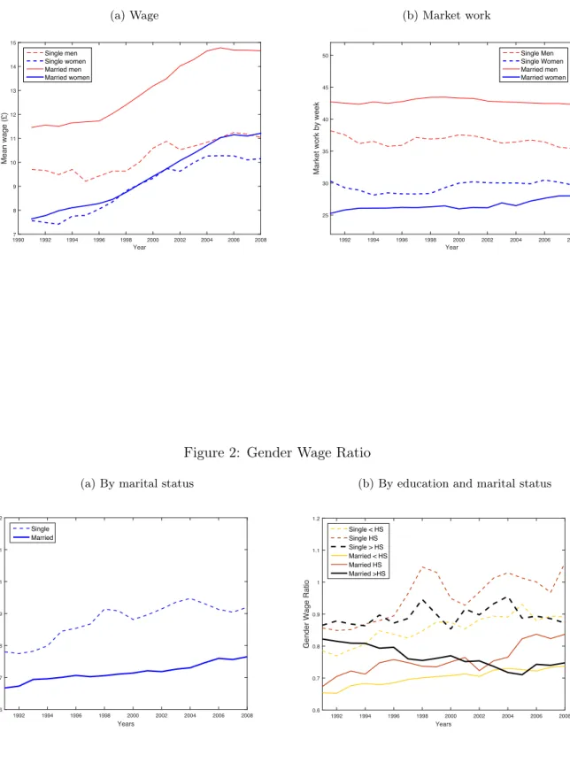
Figure 1 summarizes the main trends in labour market outcomes by gender and marital status over the 1991-2008 period. Figure 1a shows that men earn more than women, and that married individuals earn more than singles. Wages increase in the decade following 1995, and this increase is steeper for married people than for singles. By the end of the period, married women have caught up with single men but the gap between married men and women remains unchanged. Figure 1b shows that these wage changes have had little eﬀect on aggregate labour supply. The ordering in hours worked between married and single men and women remains very stable. Married males work more than single males, who work much more than single and married females. Nevertheless, by the end of the period, married women have increased labour supply by almost three hours per week, while single men have decreased labour supply by two hours.

Figure 2 shows that the female-male wage ratio has increased over those years, from 0.78 to 0.92 for singles and from 0.67 to 0.76 for married individuals. The decomposition by education in Figure 2b shows that this increase mainly concerns lower education levels. For high educated individuals, the gender wage gap has remained stable for singles and has slightly increased for married people.

Figure 3 plots the distributions of log wages among couples in 1991-92 and in 2007-2008. Wage dispersion has increased over the period, particularly for married women. The shift to the right of the distribution of married women’s wages is accompanied by an increase in the correlation of wages among couples (0.27 in 1991 and 0.35 in 2007).

Figure 4 documents the repartition of wages within couples. It plots the distributions of the female share of total household labour income (i.e. the aggregate wage) across married couples, separately for 1991-1992 and 2007-2008. The left panel displays the density and the right panel the cumulative distribution. The 2007-2008 distribution stochastically dominates the 1991-1992 distribution but not by a large extent. A slow transition toward a reduction of the gender wage gap within couples yet seems to be at work.

Finally we note that the strong increase in wages previously documented, particularly for women and married individuals, is paralleled by an increase in education for women and couples (Figure 5). Figure 6 shows the repartition of couples by both spouses’ education in 1991-92 and in 2007-08. The fraction of couples where both spouses are high-school dropouts has been divided by two. Simultaneously, the fraction of couples where both spouses have higher education has doubled during the period.

4_{We estimate a diﬀerent FVI for each year. However, between two consecutive years with no change in marital}

status, the FVI changes by less than 15% for more than 80% of individuals. This change has no clear direction and is centred around 0.

(7)

Figure 1: Wages and labour supply by gender and marital status (a) Wage Year 1990 1992 1994 1996 1998 2000 2002 2004 2006 2008 Mean wage (£) 7 8 9 10 11 12 13 14 15 Single men Single women Married men Married women (b) Market work Year 1992 1994 1996 1998 2000 2002 2004 2006 2008

Market work by week

25 30 35 40 45 50 Single Men Single Women Married men Married women

Figure 2: Gender Wage Ratio

(a) By marital status

1992 1994 1996 1998 2000 2002 2004 2006 2008 Years 0.6 0.7 0.8 0.9 1 1.1 1.2

Gender Wage Ratio

Single Married

(b) By education and marital status

1992 1994 1996 1998 2000 2002 2004 2006 2008 Years 0.6 0.7 0.8 0.9 1 1.1 1.2

Gender Wage Ratio

Single < HS Single HS Single > HS Married < HS Married HS Married >HS

(8)

Figure 3: Distribution of wages in the population (a) 1991-1992 (b) 2007-2008 Log wage 1 1.5 2 2.5 3 3.5 Density 0 0.05 0.1 0.15 Married females Single females Married males Single males Log wage 1 1.5 2 2.5 3 3.5 Density 0 0.05 0.1 0.15 Married females Single females Married males Single males Log wage 1 1.5 2 2.5 3 3.5

Cumulative Distribution Function

0 0.1 0.2 0.3 0.4 0.5 0.6 0.7 0.8 0.9 1 Married females Single females Married males Single males Log wage 1 1.5 2 2.5 3 3.5

Cumulative Distribution Function

0 0.1 0.2 0.3 0.4 0.5 0.6 0.7 0.8 0.9 1 Married females Single females Married males Single males

Figure 4: Distribution of female wage share of aggregate wage within couples ( wf

wf+wm) (a) pdf

Wife share of aggregate wage

0 0.1 0.2 0.3 0.4 0.5 0.6 0.7 0.8 0.9 1 Fraction of couples 0 0.02 0.04 0.06 0.08 0.1 0.12 0.14 0.16 0.18 0.2 1991-92 2007-08 (b) cdf

0 0.1 0.2 0.3 0.4 0.5 0.6 0.7 0.8 0.9 1

Cumulative distribution of couples

0 0.1 0.2 0.3 0.4 0.5 0.6 0.7 0.8 0.9 1 1991-92 2007-08

(9)

Figure 5: Changes in education by gender and marital status 1995 2000 2005 0 0.2 0.4 0.6 0.8 1 Single Men 1995 2000 2005 0 0.2 0.4 0.6 0.8 1 Married Men 1995 2000 2005 0 0.2 0.4 0.6 0.8 1 Single Women 1995 2000 2005 0 0.2 0.4 0.6 0.8 1 Married Women

No diploma/Middle School/ Vocational track High School Graduation Higher Education

Figure 6: Distribution of education within couples

> HS Female Education HS < HS 1991-92 > HS Male Education HS < HS 0 0.2 0.3 0.4 0.5 0.1 > HS Female Education HS < HS 2007-08 > HS Male Education HS < HS 0 0.2 0.3 0.4 0.5 0.1

(10)

3 Theoretical Framework

The aim of this paper is to perform a decomposition of the observed dynamics of household labour supply and matching patterns. We want to quantify how much of these changes results from composition changes (e.g. from a higher proportion of educated and high wage women), and how much results from changes in preferences and/or home production. To carry out this exercise we need a model. This section provides a presentation of a simplified version of the structural search and matching model of marriage with labour supply first introduced by GJR.

3.1 Overview of the model

We consider a population of individuals segmented by gender. Men and women are heterogeneous in characteristics such as education, wages and family values, assumed observable and fixed. Each unique combination of characteristics defines a type.

Single individuals randomly meet in the marriage market. There is no search during marriage. Upon meeting, they must decide whether to accept the current match or wait for a better potential partner. The overall distribution of types by gender is exogenous, but the distributions of types by gender and marital status is endogenous.

The matching decision is modelled as follows. A fraction of household resources is used to produce a public good. If two potential partners home-produce more together than separately (through task specialization, so as to give birth to children, etc.) a surplus is produced that is shared between spouses by Nash bargaining, using the value of being single as the outside option. Matching occurs if the match surplus is positive. Through Nash bargaining partners determine optimal levels of income transfers between them and also how much to save, collectively, in order to finance home production.

In the real world there is no such thing as perfect homogamy. Empirical perfect assignment models of the marriage market account for such mismatch by assuming i.i.d measurement error in the marriage surplus (Choo and Siow, 2006, Galichon and Salanié, 2012, Dupuy and Galichon, 2014). We rather consider an idiosyncratic source of heterogeneity in the match surplus that aﬀects the level of the home-produced public good. In addition, the match-specific component is subject to shocks, which is a way of endogenizing divorce. If the couple does not separate as a result of the match-specific shock, transfers may yet be renegotiated to diﬀerent levels in the same way as before.

3.2 Meetings, marriages and divorces

Types are denoted i for males and j for females, and we use the subscripts m and f to index gender. The number of individuals of each type is given by the density functions `m(i)and `f(j), with Lm =´ `m(i) diand Lf =´ `f(j) dj. Let m(i, j) denote the number of couples of a given type in the population, resulting in M = ˜ m(i, j) di dj couples in the whole population. Let nm(i), nf(j), Nm, Nf denote the corresponding densities and number of individuals for singles. These quantities are related to each other by simple accounting restrictions,

`m(i) = nm(i) + ˆ

m(i, j) dj, `f(j) = nf(j) + ˆ

(11)

We denote as m and f the rates at which male and female singles meet other singles per unit of time. The number of males meeting a female ( mNm) is equal to the number of females meeting a male ( fNf). Let = m/Nf = f/Nm. Let ↵ij denote the equilibrium probability of marriage for a male of type i meeting a female of type j. Although this probability is type-specific (through the type-dependency of partners surplus from marriage) the meeting probabilities are assumed to be the same for all individuals of a given gender. In principle, we could allow for some amount of directed search whereby high educated males would have a higher probability of meeting high educated females for example. However, if we go too far in the direction of heterogeneous meeting rates, then, absent data on dating, the separate identification of meeting/divorce rates ( and ) and matching probabilities becomes diﬃcult if not simply impossible.

For a given value of ↵ij, the number of new marriages (or cohabitations) of type (i, j) per unit of time is MF (i, j) = nm(i) m nf(j) Nf ↵ij = nf(j) f nm(i) Nm ↵ij = nm(i) nf(j) ↵ij.

It has three components: a single male of type i, out of the nm(i) identical ones, meets a single female with probability m = Nf; this woman is of type j with probability nf(j)/Nf; the marriage is consummated with probability ↵ij.

The marriage probability ↵ij is a non-degenerate probability because there exists a match-specific utility component z that is drawn from a distribution G at the first meeting. This random utility component generates heterogeneity in the matching decisions. In addition, we allow the match-specific component to be updated infrequently through i.i.d. shocks from the same distribution G according to a Poisson process with parameter . Spouses’ decision to remain together results from the updated surplus of the current match: divorce occurs if the updated value of z does no longer satisfy the matching rule. This happens with probability 1 ↵ij. The flow of (i, j) divorces per unit of time is thus equal to

DF (i, j) = m(i, j) (1 ↵ij).

Thanks to this match dissolution mechanism, the observed flow of divorce DF (i, j), and the number of (i, j) couples, m(i, j), also contribute to the identification of the matching parameters (see GJR for details). Note that this mechanism explains why many matches will end relatively quickly, the divorce rate stabilizing at a low value after the first two years of marriage.

We shall assume that the population is approximately in a steady state. This is a more reasonable approximation than it may seem at first sight. Indeed, if the flow of new marriage were vastly superior to the flow of divorces (and not death since we focus on prime age individuals) then the number of couples would grow, which is not what we see in the data (see Figure 7).

The steady state restriction imposes that flows in and out of the stocks of married couples of each type exactly balance each other out: for all (i, j), DF (i, j) = MF (i, j), or

(1 ↵ij) m(i, j) = nm(i) nf(j) ↵ij. This defines the equilibrium number of (i, j) couples as m(i, j) = ↵(i,j)

(12)

Figure 7: Shares of married and unmarried by gender 1992 1994 1996 1998 2000 2002 2004 2006 2008 Year 0 0.1 0.2 0.3 0.4 0.5 0.6 0.7 0.8 0.9 1 Share Married men Single Men Married Women Single Women

accounting restrictions (3.1), the equilibrium measures of singles are solutions to the following fixed-point system:

nm(i) = `m(i)

1 + ´ nf(j)_{1 ↵(i,j)}↵(i,j) dj

, nf(j) =

`f(j)

1 + ´ nm(i)_{1 ↵(i,j)}↵(i,j) di

. (3.2)

3.3 Preferences and home production

The instantaneous flow of utility enjoyed either as a single or as a spouse is drawn from private consumption c0 (whose price is normalized to one), private leisure e, and a public good q that is produced in-house. We normalize to one the total amount of time available per week to any individual. So market hours is h ⌘ 1 e, and wi is both the wage rate and the total income available to the individual. For simplicity, wages are assumed perfectly observable and deterministic.

Since home production is not observed, we normalize it by setting his value equal to 1 for singles. And for married couples, we assume that home production only requires some amount of market good expenditure c, namely,

q = zF_ij1(c), F_ij1(c) = Zij(c Cij)K.

The scale shifter Zij is a deterministic source of externality that only depends on spouses’ types. For identification we shall introduce type complementarities (interactions) only in the match quality parameter Zij, and not in minimal expenditure Cij.

A single of type i has his/her entire total income wi free to allocate between consumption and leisure: c0+ wie = wi. For a married couple of male-female type (i, j), we have

c0m+ wiem= wi tm ⌘ Rm, c0f + wjef = wj tf ⌘ Rf,

(13)

transfers can be negative, but not both at the same time. Transfers are a way of redistributing resources to children as well as between spouses.

Individual with exogenous characteristics i draw utility Ui(c0, e, q) from privation consump-tion, leisure and the public good. Assuming corner solutions away, we will work with the corresponding indirect utility, assumed to be of the quasi-linear form:

i(R, q)⌘ max{Ui(c0, e, q) : c0 > 0, 1 > e > 0, c0+ wie R} = q

R Ai(wi) Bi(wi)

, (3.3)

where Ai and Bi are diﬀerentiable, non-decreasing and concave functions of the wage wi and other individual characteristics such as gender and education.5 _{This specification is standard} in the labour supply literature (linear demand systems). We also normalize the denominator as Bi(1) = 1. The demands for consumption and leisure follow from the indirect utility function by application of Roy’s identity.

3.4 Marriage contracts

Transfers and the quantity of public good produced are determined by the marriage contract that spouses sign upon meeting. We assume that individuals can walk away from the negotiation at any time. Marriage contracts must thus be mutually beneficial for their whole duration. Specifically, the contract between a male of type i and a female of type j, endowed with a given draw of the current match-specific shock z, specifies a per-period utility level for both spouses, um and uf (generated using the indirect utility previously described), and two promised continuation values, V1

m(z0) and Vf1(z0), for any realization z0 of the next match-specific shock. We index u and V1 _{by subscripts m and f instead of i and j because they are at this point variables that} remain to be determined. The equilibrium solutions will be functions of types i and j.

Let Wm and Wf denote the present value of a marriage contract for any given choice of (um, uf, Vm1, Vf1), and let Vi0 and Vj0 similarly denote the value of single-hood for type-i men and type-j women. Let r denote the discount rate. The marriage values are related to the values of remaining single by the following Bellman equation:

rWm= um+ ˆ ⇥

max V_i0, V_m1(z0) Wm ⇤

dG(z0), (3.4)

The flow value of marriage is the sum of the instantaneous utility and a term that values the event of a shock to the match-specific component. With probability there is a shock and a new value z0 _{is drawn from distribution G. If the new value of marriage V}1

m(z0) is less than the value of single-hood V0

i a divorce occurs; otherwise the match continues with a new way of sharing resources.

Marriage utilities um, uf depend on optimal choices of c, tm, tf as

um = i(wi tm, q), uf = j(wj tf, q), with q = zFij1(c).

The household first determines the optimal choice of c, tm, tf by maximizing the Nash bargaining

(14)

criterion max c,tm,tf Wm Vi0 Wf Vj0 1 , (3.5)

subject to the feasibility constraint c = tm+ tf, and where is a bargaining parameter. Without commitment, the promise-keeping constraint imposes that Wm = Vm1(z). Denoting x+ _{⌘ max{x, 0}, the equilibrium surplus from marriage follows as}

(r + )⇥V_m1(z) V_i0⇤= um+ ˆ ⇥

V_m1(z0) V_i0⇤+dG(z0) rV_i0, (3.6)

with a symmetric expression for V1

f(z). Note that the equilibrium value of a marriage contract between spouses is a function of types i, j and z. We shall use the notation V1

m(i, j, z), Vf1(i, j, z) whenever necessary to make precise the dependence on i, j.

The matching probability is the probability that the participation constraint holds at the current value of (i, j, z), that is

↵ij = Pr{Vm1(z) Vi0 0 and Vf1(z) Vj0 0}. The present value of single-hood follows as

rV_i0 = i(wi, 1) + ¨ ⇥

V_m1(i, j, z) V_i0⇤

⇥ 1{Vm1(z) Vi0 0 and Vf1(z) Vj0 0} dG(z) nf(j) dj, (3.7) The continuation value is the expected value of marriage. For this a meeting must occur and the contract that results from Nash bargaining must make marriage preferable to remaining single for both dating individuals.

3.5 Equilibrium solution with transferable utility

We show in GJR that the equilibrium of this economy satisfies two important properties. First, domestic production is determined independently of transfers and continuation values (separa-bility): public good expenditures only depends on individual characteristics and preferences. Secondly, there exists a function Sij(z) measuring the surplus from marriage of a male of type i and a female of type j whose match specific draw is z. This surplus is shared between spouses and matching requires positive surplus (transferability). We summarize below the main steps of the model solution, and highlight the relationships that allow to estimate the model from observed consumption and matching patterns.

3.5.1 Equilibrium households consumption

The first order conditions of the Nash bargaining problem (3.5) with respect to domestic pro-duction are @ ln F1 ij(c) @c = K c C_ij = 1 X,

where X ⌘ wi + wj Ai Aj c is the net total private expenditure, i.e. what is left of total income wi+ wj to be spent on private consumption and leisure after spending c on home

(15)

production above and beyond the minimal expenditures Ai + Aj. Optimal home production expenditure then follows as

c(i, j) = Cij + K(wi+ wj Ai Aj)

1 + K , (3.8)

and the equilibrium values of net private expenditure and domestic production is

Xij =

wi+ wj Ai Aj Cij

1 + K , F

1

ij = ZijKKXijK. (3.9) Thanks to the multiplicative nature of the public good provision rule, these equilibrium quanti-ties only depend on individual characteristics and not on the match specific shock.

3.5.2 Surplus sharing

The match surplus results from the first-order conditions of the Nash bargaining problem (3.5) with respect to transfers,

q Bi(r + )[Vm1(z) Vi0] = q(1 ) Bj(r + )[V_f1(z) V_j0] = q Sij(z) (3.10) where Sij(z)⌘ Bi(r + )[Vm1(z) Vi0] + Bj(r + )[Vf1(z) Vj0] defines the match surplus.

Denote Sij ⌘´ Sij(z0)+dG(z0) the integrated surplus. The promise keeping constraint (3.6) implies that the match surplus satisfies the following Bellman equation:6

Sij(z) = qXij BirVi0 BjrVj0+_{r +} Sij. (3.11) The equilibrium integrated surplus then solves the fixed-point equation:

Sij = Fij1 XijG BirV_i0+ BjrV_j0 _r+ Sij F1 ijXij ! , (3.12) where G(s) ⌘ ´ (z s)+_{dG(z) =}´+1 s z dG(z) s[1 G(s)].7

These equations allow to calculate the integrated surplus and the match surplus given the values of being/remaining single. The probability that a match (i, j, z) is consummated then follows as ↵ij = Pr{Sij(z) > 0} = 1 G " G 1 Sij F1 ijXij !# . (3.13)

Finally, the value of single-hood is the sum of the utility flow of being single plus the option

6_{See GJR, Appendix A for details on the algebra.}

7_{The function G is decreasing and invertible on the support of G, with G}0₌ ₍₁ _{G). It is thus a contracting}

(16)

value of marriage. The equilibrium rent-sharing equations (3.10) imply that BirVi0= Bi 0i +_{r +} ˆ Sijnf(j) dj, BjrVj0= Bj j0+ (1 ) r + ˆ Sijnm(i) di. (3.14)

Note that the equilibrium is fully characterized by BrV0

i , BjrVj0, nm(i), and nf(j). In practice, the equilibrium is computed by iterating on equations (3.2), (3.14) until convergence, making use of equations (3.12), (3.13) to compute ↵ij and with Nm = ´ nm(i) di and Nf = ´ nf(j) dj.

Lastly, some algebra shows that equilibrium transfers tm(i, j, z) and tf(i, j, z) are a way of sharing net total private expenditure Xij:

wi Ai tm= ij(z)Xij, wj Aj tf = [1 ij(z)]Xij. (3.15) The sharing rule ij(z)depends on the bargaining parameter and the outside option (single-hood) in the following way:

ij(z) = + 1 z (1 )BirVi0 BjrVj0 F_ij1 Xij . (3.16)

This equation shows how outside options (single-hood) can move the sharing rule above or below the exogenous bargaining power level .

4 Estimation and results

The model is estimated on BHPS data. We first describe how structural components of the model depend on observables, and discuss identification.

4.1 Parametric specification

We introduce exogenous variations in the structural components of the model through several dimensions of observable heterogeneity: gender gi, education Edi, wage wiand the family values index xi. We specify preference parameters as

Ai = a0g(Edi) bg + a1g 1 bg wi+ a2g 2 bg w_i2, ln Bi = bgln wi, gi= g2 {m, f},

with a0g(Edi) = a0gH or a0gL, depending on the education indicator Edi 2 {H, L}, where L refers to high school dropout or vocational and H to higher education (high school and higher). The demand for leisure, with given transfer ti (ti = 0 for singles), thus writes:

(17)

Domestic production depends on gender, education and family values but not on wages:

Cij ⌘ C + cmH1(Edi = H) + cf H1(Edj = H) + c1mxi+ c1fxj,

where C, cmH, cf H, c1m, c1f are 5 scalar parameters and 1(Edi = H) is equal to 1 if Edi = H and 0 otherwise. Public good quality Zij is a general function of spouses’ characteristics:

Zij ⌘ Z(Edi, wi, xi, Edj, wj, xj),

that will be estimated non-parametrically. We let Zij depend on wages and on interactions be-tween male and female factors. This will allow us to estimate the source of marriage externalities that is not already accounted for by resource sharing through common funding of the public good.

Lastly, the distribution of match-specific shocks z is log-normal: G(z) = (ln(z)/ z), where is the standard normal cdf and z is the standard deviation of z. We then have

G(s) = s ✓ ln s z ◆ + e 2 z 2 ✓ ln s z + z ◆ . 4.2 Identification

We prove identification without data on domestic production inputs under the preceding para-metric specification, assuming in particular that 1) Zij depends on interactions between spouses’ types but not Cij, and 2) Cij does not depend on wages.

First, matching parameters , , ↵ij are directly inferred from observed flows by type on the marriage market. Second, preference parameters are identified from labour supply as follows. For singles, equation (4.1) takes the form:

wie0 = a0g(Edi) + (a1g+ bg)wi+ a2gw2i. (4.2) Without separate variation in income and wages, a1g + bg is identified but not a1g and bg separately. This is the usual identification issue with labour supply models. Parameters a1g and bg are not separately identified unless a source of non-earned income is observed. For married couples, the leisure equation (4.1) together with equations (3.15), (3.16) for transfers imply that

wie1m = a1m 1 bm wi+ 2a2m 2 bm w2_i + bm ij(z)Xij, wje1f = a1f 1 bf wj+ 2a2f 2 bf w2_j + bf[1 ij(z)]Xij. (4.3)

The important empirical implication of this equation is that leisure demands e1

m and e1f exhibit variations that are independent of wages. These variations come not only from the match-specific component z, but also from the interactions betweens observable spouses’ characteristics. Moreover, under the assumption that complementarities (such as interactions between spouses’ education levels) aﬀect parameter Zij but not Cij, then the net private expenditure Xij =

wi+wj Cij Ai Aj

1+K does not depend on interactions terms while ij(z) does. This restriction on individual characteristics thus generates further independent variations in the leisure equations.

(18)

Denote ⇣ one such observable interaction term, assumed continuous for simplicity.8 Diﬀer-entiating equations (4.3), with @ ij(z)/@⇣ 6= 0, we obtain an identifying restriction for bm/bf:

@(wie1m)/@⇣ @(wje1_f)/@⇣

= bm bf

. (4.4)

Next, eliminating ij(z) from equations (4.3) yields

wi bm ✓ e1_m a1m 1 bm 2a2m 2 bm wi ◆ +wj bf ✓ e1_f a1f 1 bf 2a2f 2 bf wj ◆ = Xij = wi+ wj Cij Ai Aj 1 + K . (4.5)

Assuming further that Cij does not depend on wages, one can diﬀerentiate this equation with respect to wages wiand wj and obtain two additional restrictions involving bm, bf and K (given that the other preference parameters are already identified by the leisure equations for singles). That makes three equations for three parameters that generically suﬃce for identification.

Once preference parameters and elasticity K have been identified, equation (4.5) identifies Cij. The identification of bargaining power and of the variance of the match-specific component z finally follow as in GJR.

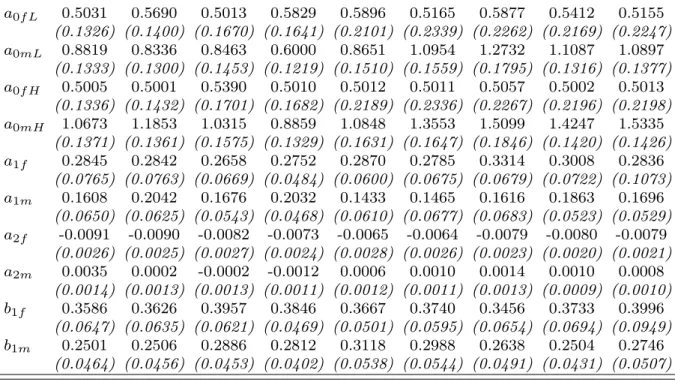
4.3 Parameter estimates

The model is separately estimated for every couple of years in the list 1991-92, 93-94, ..., 2007-08 by GMM as explained in the Appendix. The results are displayed in Table 1. The parameters driving the demand for leisure seem to increase overtime. The parameter a0strongly increases for men (particularly for educated men). There is no clear monotonic trend for the other parameters, but some slight tendency. For women, the parameter a1 slightly increases and the negative parameter a2 decreases in absolute value. Besides b1 increase for both genders. Domestic production constant cost (C) decreases overtime. On average, men’s education increases the domestic production cost whereas women’s education decreases the domestic production cost but less and less overtime. Finally, high family values decrease domestic production cost, particularly so for women, but this eﬀect seems to decrease overtime. The bargaining power coeﬃcient is estimated around 0.5, which implies that the balance of powers between spouses in the family is only function of the outside options.9

Our model delivers a non-parametric estimate of the match quality parameter Zij. This is a complex function of spouses’ wages, education and family values indices. In Table 2 we present the results of the least-square projection of ln Zij on indicators of the wage diﬀerential, and the education and family values of both spouses, including interactions. The match quality clearly and significantly decreases with the relative wage of the female spouse. At the same time, there is strong evidence of homophily in education. There are few obvious trends in the parameters. The only obvious one is for female education – educated women becoming more “attractive” over the years.

8_{Note that cross-wage interactions w}

i⇤ wjwill not work for ⇣ if they does not determine Zij.

9

z is not well estimated as we do not obtain convergence in each period (see appendix B, step 3). Instead,

(19)

Table 1: Estimated Parameters 1991 1993 1995 1997 1999 2001 2003 2005 2007 0.4806 0.4802 0.4927 0.4843 0.4815 0.4813 0.5025 0.4804 0.4847 (0.1595) (0.1722) (0.1600) (0.1453) (0.1863) (0.1621) (0.1079) (0.1147) (0.1370) Preferences a0f L 0.5031 0.5690 0.5013 0.5829 0.5896 0.5165 0.5877 0.5412 0.5155 (0.1326) (0.1400) (0.1670) (0.1641) (0.2101) (0.2339) (0.2262) (0.2169) (0.2247) a0mL 0.8819 0.8336 0.8463 0.6000 0.8651 1.0954 1.2732 1.1087 1.0897 (0.1333) (0.1300) (0.1453) (0.1219) (0.1510) (0.1559) (0.1795) (0.1316) (0.1377) a0f H 0.5005 0.5001 0.5390 0.5010 0.5012 0.5011 0.5057 0.5002 0.5013 (0.1336) (0.1432) (0.1701) (0.1682) (0.2189) (0.2336) (0.2267) (0.2196) (0.2198) a0mH 1.0673 1.1853 1.0315 0.8859 1.0848 1.3553 1.5099 1.4247 1.5335 (0.1371) (0.1361) (0.1575) (0.1329) (0.1631) (0.1647) (0.1846) (0.1420) (0.1426) a1f 0.2845 0.2842 0.2658 0.2752 0.2870 0.2785 0.3314 0.3008 0.2836 (0.0765) (0.0763) (0.0669) (0.0484) (0.0600) (0.0675) (0.0679) (0.0722) (0.1073) a1m 0.1608 0.2042 0.1676 0.2032 0.1433 0.1465 0.1616 0.1863 0.1696 (0.0650) (0.0625) (0.0543) (0.0468) (0.0610) (0.0677) (0.0683) (0.0523) (0.0529) a2f -0.0091 -0.0090 -0.0082 -0.0073 -0.0065 -0.0064 -0.0079 -0.0080 -0.0079 (0.0026) (0.0025) (0.0027) (0.0024) (0.0028) (0.0026) (0.0023) (0.0020) (0.0021) a2m 0.0035 0.0002 -0.0002 -0.0012 0.0006 0.0010 0.0014 0.0010 0.0008 (0.0014) (0.0013) (0.0013) (0.0011) (0.0012) (0.0011) (0.0013) (0.0009) (0.0010) b1f 0.3586 0.3626 0.3957 0.3846 0.3667 0.3740 0.3456 0.3733 0.3996 (0.0647) (0.0635) (0.0621) (0.0469) (0.0501) (0.0595) (0.0654) (0.0694) (0.0949) b1m 0.2501 0.2506 0.2886 0.2812 0.3118 0.2988 0.2638 0.2504 0.2746 (0.0464) (0.0456) (0.0453) (0.0402) (0.0538) (0.0544) (0.0491) (0.0431) (0.0507) Home production C 3.9363 3.7017 3.3038 4.4963 3.7167 4.1636 4.6001 4.2404 2.7159 (1.7211) (1.5909) (1.3347) (1.0997) (1.2157) (1.5382) (2.0061) (1.8102) (1.9418) c1f -0.5930 -0.6087 -0.5214 -0.7518 -0.5352 -0.5584 -0.5297 -0.5014 -0.5052 (0.2389) (0.2600) (0.2651) (0.2086) (0.2259) (0.2538) (0.2825) (0.2621) (0.2817) c1m -0.4969 -0.3636 -0.2974 -0.4311 -0.3728 -0.5189 -0.4091 -0.3754 0.1374 (0.2413) (0.2418) (0.2910) (0.2229) (0.2335) (0.2647) (0.3699) (0.3726) (0.3665) cf H -1.2049 -0.9055 -0.4120 -0.5015 -0.5362 -0.3395 -0.9060 -1.0889 -1.0400 (0.3544) (0.3250) (0.2828) (0.2528) (0.2555) (0.2651) (0.3606) (0.3350) (0.3380) cmH 0.5771 0.9064 0.1436 0.6296 0.2497 -0.0755 -0.6154 0.0579 0.6167 (0.3128) (0.3572) (0.3012) (0.2668) (0.2819) (0.3234) (0.3801) (0.3538) (0.3490) K 0.0142 0.0140 0.0214 0.0185 0.0093 0.0048 0.0080 0.0092 0.0080 (0.0691) (0.0639) (0.0561) (0.0489) (0.0446) (0.0478) (0.0614) (0.0532) (0.0601) Note. Preference parameters estimated separately for every couple of years. Standard errors in parentheses.

(20)

Table 2: Matching preferences 1991 1993 1995 1997 1999 2001 2003 2005 2007 Intercept 0.890 0.746 0.778 0.773 0.640 0.732 0.694 0.766 0.540 (0.024) (0.024) (0.020) (0.021) (0.021) (0.022) (0.024) (0.027) (0.026) h 0.25 < wf wf+wm  0.50 i -0.074 -0.022 -0.044 -0.054 -0.051 -0.054 -0.095 -0.115 -0.049 (0.007) (0.008) (0.008) (0.008) (0.008) (0.009) (0.009) (0.010) (0.011) h 0.50 < wf wf+wm  0.70 i -0.130 -0.068 -0.107 -0.114 -0.129 -0.139 -0.174 -0.173 -0.093 (0.009) (0.009) (0.009) (0.009) (0.009) (0.009) (0.010) (0.011) (0.011) h 0.70 < wf wf+wm i -0.251 -0.185 -0.270 -0.274 -0.295 -0.242 -0.287 -0.237 -0.196 (0.026) (0.021) (0.022) (0.020) (0.018) (0.020) (0.021) (0.027) (0.033) F V Im -0.156 -0.148 -0.163 -0.144 -0.134 -0.160 -0.147 -0.146 -0.072 (0.007) (0.008) (0.006) (0.006) (0.006) (0.007) (0.008) (0.009) (0.008) F V If -0.127 -0.123 -0.146 -0.133 -0.107 -0.142 -0.109 -0.113 -0.099 (0.008) (0.008) (0.007) (0.007) (0.007) (0.008) (0.008) (0.009) (0.009) F V Im⇤ F V If 0.041 0.043 0.053 0.047 0.048 0.056 0.053 0.050 0.040 (0.002) (0.002) (0.002) (0.002) (0.002) (0.002) (0.003) (0.003) (0.003) (Educm= HS) -0.095 -0.041 -0.085 -0.017 -0.024 -0.046 -0.052 -0.064 -0.013 (0.006) (0.006) (0.006) (0.006) (0.006) (0.006) (0.007) (0.008) (0.008) (Educf = HS) -0.191 -0.131 -0.074 -0.092 -0.064 0.012 0.040 0.009 -0.015 (0.009) (0.009) (0.007) (0.007) (0.007) (0.007) (0.007) (0.008) (0.009) (Educm> HS) -0.214 -0.200 -0.159 -0.152 -0.201 -0.203 -0.232 -0.216 -0.203 (0.008) (0.008) (0.007) (0.007) (0.007) (0.008) (0.009) (0.011) (0.012) (Educf > HS) -0.214 -0.181 -0.195 -0.223 -0.229 -0.189 -0.217 -0.192 -0.158 (0.012) (0.011) (0.010) (0.009) (0.009) (0.009) (0.010) (0.010) (0.010) (Educm= HS)⇤ (Educf = HS) 0.186 0.162 0.171 0.111 0.081 0.038 0.077 0.084 0.074 (0.014) (0.013) (0.011) (0.011) (0.011) (0.011) (0.012) (0.013) (0.014) (Educm> HS)⇤ (Educf > HS) 0.403 0.397 0.375 0.346 0.378 0.413 0.422 0.409 0.379 (0.016) (0.015) (0.013) (0.012) (0.012) (0.013) (0.014) (0.015) (0.016) (Educm> HS)⇤ (Educf = HS) 0.164 0.187 0.142 0.142 0.155 0.184 0.193 0.183 0.216 (0.018) (0.016) (0.013) (0.012) (0.012) (0.012) (0.013) (0.015) (0.016) (Educm= HS)⇤ (Educf > HS) 0.132 0.138 0.187 0.139 0.103 0.123 0.148 0.131 0.118 (0.018) (0.017) (0.015) (0.013) (0.013) (0.014) (0.014) (0.015) (0.015) R2 0.51 0.39 0.44 0.41 0.50 0.42 0.49 0.40 0.32

(21)

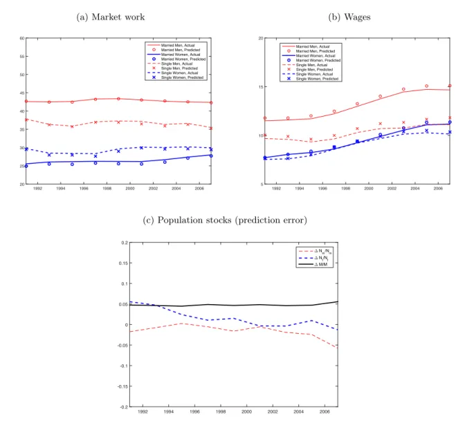
Figure 8: Fit of market work trends and wage trends

(a) Market work

1992 1994 1996 1998 2000 2002 2004 2006 20 25 30 35 40 45 50 55 60

Married Men, Actual Married Men, Predicted Married Women, Actual Married Women, Predicted Single Men, Actual Single Men, Predicted Single Women, Actual Single Women, Predicted

(b) Wages 1992 1994 1996 1998 2000 2002 2004 2006 5 10 15 20

(c) Population stocks (prediction error)

1992 1994 1996 1998 2000 2002 2004 2006 -0.2 -0.15 -0.1 -0.05 0 0.05 0.1 0.15 0.2 ∆ N m/Nm ∆ N f/Nf ∆ M/M 4.4 Model fit

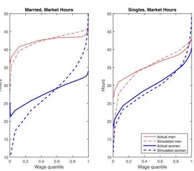
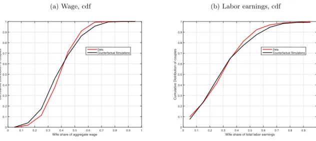
Starting from random initial distributions of single and couples in the population, we simulate the equilibrium and predict the distributions of characteristics among couples and singles and labour supplies. Our model performs well in predicting the average labour supplies of men and women by marital status over the period (Figure 8). The model also predicts the equilibrium number of singles and couples with less than 5% of error for each period. Finally the prediction of working hours conditionally on wages and education is also quite good (Figure 9), and so is the fit of the distribution of female relative earnings and wages (Figure 10).

4.5 Counterfactual analysis

We now turn to the main empirical question of the paper: what are the main components of the changes in labour supply and sorting shown in Section 2? Three main factors and their evolutions can explain these changes: the distributions of characteristics in the population of males and females (in particular, wages and education); preferences and home production; and

(22)

Figure 9: Market work simulations in 2007-08

(a) Conditional on wage quantile

Wage quantile 0 0.2 0.4 0.6 0.8 1 Hours 10 15 20 25 30 35 40 45

50 Married, Market Hours

50 Singles, Market Hours

Actual men Simulated men Actual women Simulated women

(b) Conditional on education level

Education level 1 1.5 2 2.5 3 Hours 10 15 20 25 30 35 40 45

(23)

Figure 10: Fit of distribution of female spouse’s share of total labour earnings and wages in 2007-08

(a) Wage, cdf

0 0.1 0.2 0.3 0.4 0.5 0.6 0.7 0.8 0.9 1

Cumulative Distribution of couples

0 0.1 0.2 0.3 0.4 0.5 0.6 0.7 0.8 0.9 1 Data Counterfactual Simulations (b) Labor earnings, cdf

Wife share of total labor earnings

0 0.1 0.2 0.3 0.4 0.5 0.6 0.7 0.8 0.9 1

Cumulative Distribution of couples

0 0.1 0.2 0.3 0.4 0.5 0.6 0.7 0.8 0.9 1 Data Counterfactual Simulations

public good quality.

To separately identify the specific contribution of each one of these factors, we run three counterfactual experiments. In the first experiment, we fix Zij at its estimated 1991 value and we simulate a new equilibrium for each two-year observation sample between 1991 and 2008 (the other parameters being set equal to their estimated values in all years). In the second counterfactual simulation, we let Zij vary according to its estimated value in each year and we keep all other parameters fixed at their 1991 values. In the last experiment, only composition eﬀects are allowed for (changes in the exogenous distributions of exogenous characteristics).

The remaining figures of the paper clearly show that preferences are responsible for the observed changes in labour supply, and public good quality accounts for the changes in marriage sorting. Without the estimated variation in Zij (Figures 11, 12) there are fewer marriages and the number of singles tends to be overestimated. Moreover, the wages of married men and women are well predicted, but the wages of singles are overestimated. This is because there is more education complementarity in 2007 than in 1991. So with the 1991 parameters we simulate fewer marriages between high educated individuals. Consequently, the wages of singles increase. Without the estimated variations in the preference parameters (Figures 13, 14), the labour market supply of women and single men would be much higher than observed. A look at Table 1 shows that the preference for leisure has increased over time for both men and women. Lastly, if we fix all parameters (preferences and public good quality), we obtain the worst of the two worlds (figures available upon request).

(24)

Figure 11: Counterfactual trends

(All parameters vary; but Zij stays at 1991 level)

(a) Market work

1992 1994 1996 1998 2000 2002 2004 2006 20 25 30 35 40 45 50 55 60

(b) Wage 1992 1994 1996 1998 2000 2002 2004 2006 5 10 15 20

(c) Population stocks 1992 1994 1996 1998 2000 2002 2004 2006 -0.2 -0.15 -0.1 -0.05 0 0.05 0.1 0.15 0.2 ∆ N_m/N_m ∆ N_f/N_f ∆ M/M

(25)

Figure 12: Counterfactual market hours in 2007-08 (All parameters vary; but Zij stays at 1991 level)

(a) Market work conditional on wage quantile

(b) Market work conditional on education level

(26)

Figure 13: Counterfactual trends

(Only Zij varies; all other parameters remain fixed at 1991 value)

(a) Market work

1992 1994 1996 1998 2000 2002 2004 2006 20 25 30 35 40 45 50 55 60

(b) Wages 1992 1994 1996 1998 2000 2002 2004 2006 5 10 15 20

(c) Population stocks 1992 1994 1996 1998 2000 2002 2004 2006 -0.2 -0.15 -0.1 -0.05 0 0.05 0.1 0.15 0.2 ∆ N_m/N_m ∆ N_f/N_f ∆ M/M

(27)

Figure 14: Counterfactual market hours in 2007-08

(Only Zij varies; all other parameters remain fixed at 1991 value)

(a) Market work conditional on wage quantile

(b) Market work conditional on education level

(28)

5 Conclusion

In this paper, we have developed a version of GJR’s search-matching model of the marriage market with labour supply but without home production time inputs. We derive conditions under which the marriage and household labour supply model remains identified. We estimate the model using GMM on data drawn from the British Household Panel Survey, 1991-2008, and we allow preference parameters to evolve over the observation period. We show that the preference for leisure of men should change over time in order to fit the observed dynamics in labour supply. We also need to allow for changes in the strength of homophily (in particular with respect to spouses’ education) in order to explain the observed changes in sorting. As GJR obtain a good fit of the data with time-invariant parameters, we conclude that it is important to model family labour supply in conjunction with time spent in home production.

Many labour market policies condition benefits on marital status and the number of children. This requires a non trivial extension of the model, but one that should be high on the agenda. Also, one critical assumption that we make in this paper is the time invariance of wages. However, it is likely that many interesting features of the marriage market could be better fitted with wages varying with age and subject to stochastic shocks. Such an extension is desirable yet also non trivial as it will make the model non stationary.

Appendix - Estimation algorithm

Let us consider one two-year cross-section of household data on time uses, gender, wages, family values and education. We use couples of years to increase sample size. In this section, the index i refers to an observation unit of the sample of male singles, j refers to female singles, and (i, j) refers to couples. For singles, we observe labour supply h0

i and education Edi 2 {L, H}, wages wi and family values indices

xi. For couples, the corresponding time use observations are h1mij and h1f ij. Leisure is e = 1 h. The

estimation procedure is iterative and goes through the following steps.

1. Estimate , , ↵ij from non-parametric estimates of stock densities nm(i), nf(j), m(i, j)and

corre-sponding flows as described in GJR.

2. Given a value for z, estimate the parameters of preferences and domestic productions, as well as

bargaining power , by two-stage GMM first with metric equal to the identity matrix and second with metric equal to the diagonal of the inverse of variance-covariance matrix of moments. GMM are based on the following residuals and instruments:

(a) For single men, the residuals are u0

i = e0i a0m(Edi)/wi a1m a2mwi bm,

with a similar expression for single women. The instruments are ⇠i= (1, 1(Edi= H), xi, wi, 1(Edi = H)/wi) .

(29)

(b) For couples, the residuals are u1ij = e1 mij 1 ba1mm 2a2m 2 bmwi bm ijXij/wi e1 f ij a1f 1 bf 2a2f 2 bfwj bf(1 ij)Xij/wj ! , with Xij= wi+ wj Cij Ai Aj 1 + K , ij= +E ✓₁ z|z G 1₍₁ _↵ ij) ◆₍₁ _)B irVi0 BjrVj0 F1 ijXij .

The instruments are ⇠i⌦ ⇠j. The leisure residuals follow from equations (4.3), (3.15), after

taking the expectation with respect to z. Note that the distribution of z ⇠ LN (0, 2

z)implies that E 1 z|z > s = e 2 z 2 ⇣ ln s z z ⌘

/ ⇣ ln s_z⌘and that marriage is consummated if z G 1₍₁ _↵

ij)for the marriage probability to be equal to ↵ij. We back out Sij, BirVi0, BjrVj0

and F1

ijXij from matching probabilities ↵ij, given type densities nm(i), nf(j)and the other

parameters, by solving a fixed-point system similar to the equilibrium system in Section 3.5. For a more detailed description of this step, see GJR.

3. Estimate z by fitting the variance-covariance matrix of market hours for couples. Then repeat

steps 2 and 3 until numerical convergence.

4. Lastly, estimate public good quality Zij from (3.9):

Zij = Fij1Xij⇥KKXij1+K

⇤ 1

.

Once the model has been estimated, an economy can be simulated by computing the equilibrium as indicated in Section 3.5. Specifically, for every two-year cross section, given estimated parameters and the observed distributions of male and female types in the population (i.e. `m(i), `f(j)), we use the

equilibrium fixed point to calculate conditional distributions nm(i), nf(j), m(i, j) together with values

Sij, BirVi0, BjrVj0. Note that individual types comprise one continuous variable, the wage, and the

family values index is approximately continuous as it is constructed by aggregation of many discrete variables. Hence, functions Sij, BirVi0, BjrVj0, nm(i), nf(j), m(i, j) have to be discretized and integrals

in equilibrium operators have to be approximated. We rely for that on Clenshaw-Curtis quadrature and Chebyshev polynomials.

References

Amuedo-Dorantes, C., and S. Grossbard (2007): “Cohort-level sex ratio eﬀects on women’s labor force participation,” Review of Economics of the Household, 5(3), 249–278.

Becker, G. S. (1981): A Treatise on the Family. Harvard University Press, Cambridge (MA).

Blundell, R., M. C. Dias, C. Meghir, and J. Shaw (2016): “Female labour supply, human capital and welfare reform,” Econometrica, 84(5), 1705–1753.

Breen, R., and L. Salazar (2011): “Educational Assortative Mating and Earnings Inequality in the United States,” American Journal of Sociology, 117(3), 808–843.

Brien, M. J. (1997): “Racial Diﬀerences in Marriage and the Role of Marriage Markets,” Journal of Human Resources, 32(4), 741–778.

Chiappori, P.-A. (1988): “Rational Household Labor Supply,” Econometrica, 56(1), 63–90.

(1992): “Collective Labor Supply and Welfare,” Journal of Political Economy, 100(3), 437–467. Chiappori, P.-A., B. Fortin, and G. Lacroix (2002): “Marriage market, divorce legislation, and

(30)

Chiappori, P.-A., M. Iyigun, and Y. Weiss (2009): “Investment in Schooling and the Marriage Market,” American Economic Review, 99(5), 1689–1713.

Choo, E., and A. Siow (2006): “Who Marries Whom and Why,” Journal of Political Economy, 114(1), 175–201.

Del Boca, D., and C. J. Flinn (2005): “Household Time Allocation and Modes of Behavior: A Theory of Sorts,” IZA DP, (1821).

Dupuy, A., and A. Galichon (2014): “Personality Traits and the Marriage Market,” Journal of Political Economy, 122(6), 1271–1319.

Eika, L., M. Mogstad, and B. Zafar (2014): “Educational Assortative Mating and Household Income Inequality,” National Bureau of Economic Research Working Paper Series, No. 20271.

Eissa, N., and H. W. Hoynes (2004): “Taxes and the labor market participation of married couples: the earned income tax credit,” Journal of Public Economics, 88(9-10), 1931–1958.

Fernandez, R., N. Guner, and J. Knowles (2005): “Love and Money: A Theoretical and Empirical Analysis of Household Sorting and Inequality,” Quarterly Journal of Economics, 120(1), 273–344. Galichon, A., and B. Salanié (2012): “Cupid’s Invisible Hand: Social Surplus and Identification in

Matching Models,” Sciences Po publications info:hdl:2441/5rkqqmvrn4t, Sciences Po.

Goussé, M., N. Jacquemet, and J.-M. Robin (2016): “Marriage, Labor Supply, and Home Produc-tion,” CIRPEE WP, 2015-68.

Greenwood, J., N. Guner, G. Kocharkov, and C. Santos (2014a): “Corrigendum to Marry Your Like: Assortative Mating and Income Inequality,” American Economic Review, 104(5).

(2014b): “Marry Your Like: Assortative Mating and Income Inequality,” American Economic Review, 104(5), 348–53.

Grossbard-Shechtman, S. (1993): On the Economics of Marriage: A Theory of Marriage, Labor, and Divorce. Westview Press.

Grossbard-Shechtman, S. A. (1984): “A Theory of Allocation of Time in Markets for Labour and Marriage,” Economic Journal, 94(376), 863–82.

Lundberg, S. J., R. A. Pollak, and T. J. Wales (1997): “Do Husbands and Wives Pool Their Resources? Evidence from the United Kingdom Child Benefit,” Journal of Human Resources, 32(3), 463–480.

Seitz, S. (2009): “Accounting for Racial Diﬀerences in Marriage and Employment,” Journal of Labor Economics, 27(3), 385–437.

Shimer, R., and L. Smith (2000): “Assortative Matching and Search,” Econometrica, 68(2), 343–369.