HAL Id: hal-01400883
https://hal.inria.fr/hal-01400883
Submitted on 22 Nov 2016
HAL is a multi-disciplinary open access
archive for the deposit and dissemination of
sci-entific research documents, whether they are
pub-lished or not. The documents may come from
teaching and research institutions in France or
abroad, or from public or private research centers.
L’archive ouverte pluridisciplinaire HAL, est
destinée au dépôt et à la diffusion de documents
scientifiques de niveau recherche, publiés ou non,
émanant des établissements d’enseignement et de
recherche français ou étrangers, des laboratoires
publics ou privés.
Infinitary Lambda Calculi from a Linear Perspective
Ugo Dal Lago
To cite this version:
Ugo Dal Lago. Infinitary Lambda Calculi from a Linear Perspective. Logic in Computer Science, Jul
2016, New York, United States. �10.1145/2933575.2934505�. �hal-01400883�
Infinitary Lambda Calculi from a Linear Perspective
(Long Version)
Ugo Dal Lago
∗Abstract
We introduce a linear infinitary λ-calculus, called `Λ∞, in which two exponential modalities
are available, the first one being the usual, finitary one, the other being the only construct interpreted coinductively. The obtained calculus embeds the infinitary applicative λ-calculus and is universal for computations over infinite strings. What is particularly interesting about `Λ∞, is that the refinement induced by linear logic allows to restrict both modalities so as to
get calculi which are terminating inductively and productive coinductively. We exemplify this idea by analysing a fragment of `Λ built around the principles of SLL and 4LL. Interestingly, it enjoys confluence, contrarily to what happens in ordinary infinitary λ-calculi.
1
Introduction
The λ-calculus is a widely accepted model of higher-order functional programs—it faithfully captures functions and their evaluation. Through the many extensions introduced in the last forty years, the λ-calculus has also been shown to be a model of imperative features, control [25], etc. Usually, this requires extending the class of terms with new operators, then adapting type systems in such a way that “good” properties (e.g., confluence, termination, etc.), and possibly new ones, hold.
This also happened when potentially infinite structures came into play. Streams and, more generally, coinductive data have found their place in the λ-calculus, following the advent of lazy data structures in functional programming languages like Haskell and ML. By adopting lazy data structures, the programmer has a way to represent infinity by finite means, relying on the fact that data are not completely evaluated, but accessed “on-demand”. In presence of infinite structures, the usual termination property takes the form of productivity [9]: even if evaluating a stream expression globally takes infinite time, looking for the next symbol in it takes finite time.
All this has indeed been modelled in a variety of ways by enriching λ-calculi and related type theories. One can cite, among the many different works in this area, the ones by Parigot [26], Raffalli [27], Hughes at al. [16], or Abel [1]. Terms are finite objects, and the infinite nature of streams is modelled through a staged inspection of so-called thunks. The key ingredient in obtaining productivity and termination is usually represented by sophisticated type systems.
There is also another way of modelling infinite structures in λ-calculi, namely infinitary rewriting, where both terms and reduction sequences are not necessarily finite, and as a consequence infinity is somehow internalised into the calculus. Infinitary rewriting has been studied in the context of various concrete rewrite systems, including first-order term rewriting [18], but also systems of higher-order rewriting [20]. In the case of λ-calculus [19], the obtained model is very powerful, but does not satisfy many of the nice properties its finite siblings enjoy, including confluence and finite developments, let alone termination and productivity (which are anyway unexpected in the absence of types).
In this paper, we take a fresh look at infinitary rewriting, through the lenses of linear logic [13]. More specifically, we define an untyped, linear, infinitary λ-calculus called `Λ∞, and study its basic
properties, how it relates to Λ∞ [19], and its expressive power. As expected, incepting linearity does not allow by itself to solve any of the issues described above: `Λ∞embeds Λ001, a subsystem of Λ∞, and as such does not enjoy confluence. On the other hand, linearity provides the right tools to control infinity: we delineate a simple fragment of `Λ∞which has all the good properties one can expect, including productivity and confluence. Remarkably, this is not achieved through types, but rather by purely structural constraints on the way copying is managed, which is responsible for its bad behaviour. Expressivity, on the other hand, is not sacrificed.
1.1
Linearity vs. Infinity
The crucial rˆole linearity has in this paper can be understood without any explicit reference to linear logic as a proof system, but through a series of observations about the usual, finitary, λ-calculus. In any λ-term M , the variable x can occur free more than once, or not at all. If the variable x occurs free exactly once in M whenever we form an abstraction λx.M , the λ-calculus becomes strongly normalising: at any rewrite step the size of the term strictly decreases. On the other hand, the obtained calculus has a poor expressive power and, in this form, is not the model of any reasonable programming language. Let duplication reappear, then, but in controlled form: besides a linear abstraction λx.M , (which is well formed only if x occurs free exactly once in M ) there is also a nonlinear abstraction λ!x.M , which poses no constraints on the number of times x occurs in M . Moreover, and this is the crucial step, interaction with a nonlinear abstraction is restricted: the argument to a nonlinear application must itself be marked as duplicable (and erasable) for β to fire. This is again implemented by enriching the category of terms with a new construct: given a term M , the box !M is a duplicable version of M . Summing up, the language at hand, call it `Λ, is built around applications, linear abstractions, nonlinear abstractions, and boxes. Moreover, β-reduction comes in two flavours:
(λx.M )N → M {x/N }; (λ!x.M )!N → M {x/N }.
What did we gain by rendering duplicating and erasing operations explicit? Not much, apparently, since pure λ-calculus can be embedded into `Λ in a very simple way following the so-called Girard’s translation [13]: abstractions become nonlinear abstractions, and any application M N is translated into M !N . In other words, all arguments can be erased and copied, and we are back to the world of wild, universal, computation. Not everything is lost, however: in any nonlinear abstraction λ!x.M , x can occur any number of times in M , but at different depths: there could be linear occurrences of x, which do not lie in the scope of any box, i.e., at depth 0, but also occurrences of x at greater depths. Restricting the depths at which the bound variable can occur in nonlinear abstractions gives rise to strongly normalising fragments of `Λ. Some of them can be seen, through the Curry-Howard correspondence, as subsystems of linear logic characterising complexity classes. This includes light linear logic [15], elementary linear logic [8] or soft linear logic [21]. As an example, the exponential discipline of elementary linear logic can be formulated as follows in `Λ: for every nonlinear abstraction λ!x.M all occurrences of x in M are at depth 1. Noticeably, this gives rise to a characterisation of elementary functions. Similarly, soft linear linear can be seen as the fragment of `Λ∞ in which all occurrences of x (if more than one) occur at depth 0 in any nonlinear abstraction λ!x.M .
But why could all this be useful when rewriting becomes infinitary? Infinitary λ-terms [19] are nothing more than infinite terms defined according to the grammar of the λ-calculus. In other words, one can have a term M such that M is syntactically equal to λx.xM . Evaluation can still be modelled through β-reduction. Now, however, reduction sequences of infinite length (sometime) make sense: take Y (λx.λy.yx), where Y is a fixed point combinator. It rewrites in infinitely many steps to the infinite term N such that N = λy.yN . Are all infinite reduction sequences acceptable? Not really: an infinite reduction sequence is said to converge to the term M only if, informally, any finite approximation to M can be reached along a finite prefix of the sequence. In other words, reduction should be applied deeper and deeper, i.e., the depth of the fired redex should tend to infinity. But how could one define the depth of a subterm’s occurrence in a given term? There are
many alternatives here, since, informally, one can choose to let the depth increase (or not) when entering the body of an abstraction or any of the two arguments of an application. Indeed, eight different calculi can be formed, each with different properties. For example, Λ001 is the calculus in which the depth only increases while entering the argument position in applications, while in Λ100 the same happens when crossing abstractions. The choice of where the depth increases is crucial not only when defining infinite reduction sequences, but also when defining terms, whose category is obtained by completing the set of finite terms with respect to a certain metric. So, not all infinite terms are well-formed. In Λ001, as an example, the term M = xM is well-formed, while M = λx.M is not. In Λ100, the opposite holds. In all the obtained calculi, however, many of the properties one expects are not true: the Complete Developments Theorem (i.e. the infinitary analogue of the Finite Complete Theorem [4]) does not hold and, moreover, confluence fails except if formulated in terms of so-called B¨ohm reduction [19]. The reason is that Λ∞is even wilder than Λ: various forms of infinite computations can happen, but only some of them are benign. Is it that linearity could help in taming all this complexity, similarly to what happens in the finitary case? This paper gives a first positive answer to this question.
1.2
Contributions
The system we will study in the rest of this paper, called `Λ∞, is obtained by incepting ideas from infinitary calculi into `Λ. Not one but two kinds of boxes are available in `Λ∞, and the depth increases only while crossing boxes of the second kind (called coinductive boxes), while boxes of the first kind (dubbed inductive) leave the depth unchanged. As a consequence, boxes are as usual the only terms which can be duplicated and erased, but they are also responsible for the infinitary nature of the calculus: any term not containing (coinductive) boxes is necessarily finite. Somehow, the depths in the sense of Λ∞ and of `Λ coincide.
Besides introducing `Λ∞ and proving its basic properties, this paper explores the expressive power of the obtained computational model, showing that it suffers from the same problems affecting Λ∞, but also that it has precisely the same expressive power as that of Type-2 Turing machines, the reference computational model of so-called computable analysis [31].
The most interesting result among those we give in this paper consists in showing that, indeed, a simple fragment of `Λ∞, called `Λ4S∞, is on the one hand flexible enough to encode streams and guarded recursion on them, and on the other guarantees productivity. Remarkably, confluence holds, contrary to what happens for `Λ∞. Actually, `Λ4S∞ is defined around the same principles which lead to the definition of light logics. Each kind of box, however, follows a distinct discipline: inductive boxes are handled as in Lafont’s SLL [21], while coinductive boxes follow the principles of 4LL [8], hence the name of the calculus. So far, the 4LL’s exponential discipline has not been shown to have any computational meaning: now we know that beyond it there is a form of guarded corecursion.
2
`Λ
∞and its Basic Properties
In this section, we introduce a linear infinitary λ-calculus called `Λ∞, which is the main object of study of this paper. Some of the dynamical properties of `Λ∞ will be investigated. Before defining `Λ∞, some preliminaries about formal systems with both inductive and coinductive rules will be given.
2.1
Mixing Induction and Coinduction in Formal Systems
A formal system over a set of judgments S is given by a finite set of rules, all of them having one conclusions and an arbitrary finite number of premises. The rules of a mixed formal system S are of two kinds: those which are to be interpreted inductively and those which are to be interpreted coinductively. To distinguish between the two, inductive rules will be denoted as usual, with a
single line, while coinductive rules will be indicated as follows:
` A1 . . . ` An
` B . Intuitively, any correct derivation in such a system is an infinite tree built following inductive and coinductive rules where, however, any infinite branch crosses coinductive rule instances infinitely often. In other words, there cannot be any infinite branch where, from a certain point on, only inductive rules occur.
Formally, the set CSof derivable assertions of a mixed formal system S over the set of judgments S can be seen as the greatest fixpoint of the function IS◦ CS where CS : P(S) → P(S) is the monotone function induced by the the application of a single coinductive rule, while IS is the function induced by the application of inductive rules an arbitrary but finite number of times. IS can itself be obtained as the least fixpoint of a monotone functional on the space of monotone functions on P(S). The existence of CS can be formally justified by Knaster-Tarski theorem, since all the involved spaces are complete lattices, and the involved functionals are monotone. This is, by the way, very close to the approach from [10]. Let P(S) P(S) be the set of monotone functions on the powerset P(S). A relation v on P(S) P(S) can be easily defined by stipulating that F v G iff for every X ⊆ S it holds that F (X) ⊆ G(X). The structure (P(S) P(S), v) is actually a complete lattice, because:
• The relation v is a partial order. In particular, antisymmetry is a consequence of function extensionality: if for every X, both F (X) ⊆ G(X) and G(X) ⊆ F (X), then F and G are the same function.
• Given a set of monotone functions X , its lub and sup exist and are the functions F, G : P(S) P(S) such that for every X ⊆ S,
F (X) = \ H∈X
H(X); G(X) = [ H∈X
H(X).
It is easy to verify that F is monotone, that it minorises X , and that it majorises any minoriser of X . Similarly for G.
The function IS is the least fixpoint of the monotone functional F on P(S) P(S) defined as follows: to every function F , F associates the function G obtained by feeding F with the argument set X, and then applying one additional instance of inductive rules from S. Since (P(S) P(S), v) is a complete lattice, IS is guaranteed to exist.
Formal systems in which all rules are either coinductively or inductively interpreted have been studied extensively (see, e.g. [22]). Our constructions, although relatively simple, do not seem to have appeared before at least in this form. The conceptually closest work is the one by Endrullis and coauthors [10].
How could we prove anything about CS? How should we proceed, as an example, when tyring to prove that a given subset X of S is included in CS? Fixed-point theory tells us that the correct way to proceed consists in showing that X is (IS◦ CS)-consistent, namely that X ⊆ IS(CS(X)). We will frequently apply this proof strategy in the following.
2.2
An Infinitary Linear Lambda Calculus
Preterms are potentially infinite terms built from the following grammar:
M, N ::= x
|
M M|
λx.M|
λ ↓ x.M|
λ ↑ x.M|
↓ M|
↑ M,where x ranges over a denumerable set V of variables. T is the set of preterms. The notion of capture-avoiding substitution of a preterm M for a variable x in anoter preterm N , denoted
↓ Θ, ↑ Ξ, x ` x (vl) ↓ Θ, ↑ Ξ, ↓ x ` x (vi) ↓ Θ, ↑ Ξ, ↑ x ` x (vc) Γ, ↓ Θ, ↑ Ξ ` M ∆, ↓ Θ, ↑ Ξ ` N Γ, ∆, ↓ Θ, ↑ Ξ ` M N (a) Γ, x ` M Γ ` λx.M (ll) Γ, ↓ x ` M Γ ` λ ↓ x.M (li) Γ, ↑ x ` M Γ ` λ ↑ x.M (lc) ↓ Θ, ↑ Ξ ` M ↓ Θ, ↑ Ξ `↓ M (mi) ↓ Θ, ↑ Ξ ` M ↓ Θ, ↑ Ξ `↑ M (mc)
Figure 1: `Λ∞: Well-Formation Rules.
↓ y ` y (vc) π . ↓ y ` M ↓ y `↑ M (mc) ↓ y ` M (a) ρ . ∅ ` N (λx.x) x ` x (vl) ∅ ` λx.x (ll) ∅ ` N (λx.x) (a)
Figure 2: `Λ∞: Example Derivation Trees π (left) and ρ (right).
N {x/M }, can be defined, this time by coinduction, on the structure of N : (x){x/M } = M ;
(y){x/M } = y;
(λx.L){y/M } = λx.L{y/M }; if x 6∈ FV (M ) (λ ↓ x.L){y/M } = λ ↓ x.L{y/M }; if x 6∈ FV (M ) (λ ↑ x.L){y/M } = λ ↑ x.L{y/M }; if x 6∈ FV (M )
(LP ){y/M } = (L{y/M })(P {y/M }); (↓ L){y/M } =↓ (L{y/M });
(↑ L){y/M } =↑ (L{y/M }).
Observe that all the equations above are guarded, so this is a well-posed definition. An inductive (respectively, coinductive) box is any preterm in the form ↓ M (respectively, ↑ M ).
Please notice that any (guarded) equation has a unique solution over preterms. As an example, M = λx.M , N = N (λx.x), and M = y ↑ M all have unique solutions. In other words, infinity is everywhere. Only certain preterms, however, will be the objects of this study. To define the class of “good” preterms, simply called terms, we now introduce a mixed formal system. An environment Γ
is simply a set of expressions (called patterns) in one the following three forms: p ::= x
|
↓ x|
↑ x,where any variable occurs in at most one pattern in Γ. If Γ and ∆ are two disjoint environments, then Γ, ∆ is their union. An environment is linear if it only contains variables. Linear environments are indicated with metavariables like Θ or Ξ. A term judgment is an expression in the form Γ ` M where Γ is an environment and M is a term. A term is any preterm M for which a judgment Γ ` M can be derived by the formal system `Λ∞, whose rules are in Figure 1. Please notice that (mc) is coinductive, while all the other rules are inductive. This means that on terms, differently from preterms, not all recursive equations have a solution, anymore. As an example M = y ↑ M is a term: a derivation π for ↓ y ` M can be found in Figure 2. π is indeed a well-defined derivation because although infinite, any infinite path in it contains infinitely many occurrences of (mc). If we try to proceed in the same way with the preterm N = N (λx.x), we immediately fail: the only candidate derivation ρ looks like the one in Figure 2 and is not well-defined (it contains a “loop” of
inductive rule instances). We write T`Λ∞(Γ) for the set of all preterms M such that Γ ` M . The
union of T`Λ∞(Γ) over all environments Γ is denoted simply as T`Λ∞.
Some observations about the rˆole of environments are now in order: If x, Γ ` M , then x necessarily occurs free in M , but exactly once and in linear position (i.e. not in the scope of any box). If, on the other hand, ↓ x, Γ ` M , then x can occur free any number of times, even infinitely often, in M . Similarly when ↑ x, Γ ` M . Observe, in this respect, that inductive and coinductive boxes are actually very permissive: if ↓ x, Γ ` M , x can even occur in the scope of coinductive boxes, while x can occur in the scope of inductive boxes if ↑ x, Γ ` M . We claim that this is source of the great expressive power of the calculus, but also of its main defects (e.g. the absence of confluence).
Sometimes it is useful to denote symbols ↓ and ↑ in a unified way. To that purpose, let B be the set {0, 1} of binary digits, which is ranged over by metavariables like a or b. l0stands for ↓, while l1 is ↑. For every s ∈ B∗, we can define s-contexts, ranged over by metavariables like Csand Ds, as follows, by induction on s:
Cε::= [·]; C0·s::=↓ Cs; C1·s::=↑ Cs; Cs::= CsM
|
M Cs|
λx.Cs|
λ ↓ x.Cs|
λ ↑ x.Cs.Given any subset X of B∗, an X-context, sometime denoted as CX is an s-context where s ∈ X. A context C is simply any s-context Cs. For every natural number n ∈ N, n• is the set of those strings in B∗ in which 1 occurs precisely n times. For every n, the language n• is regular.
2.3
Finitary and Infinitary Dynamics
In this section, notions of finitary and infinitary reduction for `Λ∞are given. Basic reduction is a binary relation 7→⊆ T × T defined by the following three rules (where, as usual, M 7→ N stands for (M, N ) ∈ 7→):
(λx.M )N 7→ M {x/N }; (λ ↓ x.M ) ↓ N 7→ M {x/N }; (λ ↑ x.M ) ↑ N 7→ M {x/N }.
Basic reduction can be applied in any s-context, giving rise to a ternary relation →⊆ T × B∗× T, simply called reduction. That is defined by stipulating that (M, s, N ) ∈→ iff there are a s-context Cs and two terms L and P such that L 7→ P , M = Cs[L], and N = Cs[P ]. In this case, the reduction step is said to occur at level s and we write M →sN and level (M →sN ) = s. We often employ the notation →X, i.e., →X is the union of the relations →s for all s ∈ X. If M →sN but we are not interested in the specific s, we simply write M → N . If M →n•N , then reduction is
said to occur at depth n.
Given X ⊆ B∗, a X-normal form is any term M such that whenever (M, s, N ), it holds that s 6∈ X. The set of all X-normal forms is denoted as NFs(X). In the just introduced notations, the singleton s is often used in place of {s} if this does not cause any ambiguity. A normal form is simply a B∗-normal form.
Depths and levels have a different nature: while the depth increases only when entering a coinductive box, the level changes while entering any kind of box, and this is the reason why levels are binary strings rather than natural numbers.
Since M {x/N } is well-defined whenever M and N are preterms, reduction is certainly closed as a relation on the space of preterms. That it is also closed on terms is not trivial. First of all, substitution lemmas need to be proved for the three kinds of patterns which possibly appear in environments. The first of these lemmas concerns linear variables:
Lemma 1 (Substitution Lemma, Linear Case). If Γ, x, ↓ Θ, ↑ Ξ ` M and ∆, ↓ Θ, ↑ Ξ ` N , then it holds that Γ, ∆, ↓ Θ, ↑ Ξ ` M {x/N }.
Proof. We can prove that the following subset X of judgments is consistent with `Λ∞: n
Γ, ∆, ↓ Θ, ↑ Ξ ` M {x/N }
|
Γ, x, ↓ Θ, ↑ Ξ ` M ∈ C`Λ∞∧ ∆, ↓ Θ, ↑ Ξ ` N ∈ C`Λ∞o
Suppose that J = Γ, ∆, ↓ Θ, ↑ Ξ ` M {x/N } is in X. If J ∈ C`Λ∞, then of course
J ∈ I`Λ∞(C`Λ∞(C`Λ∞)) ⊆ I`Λ∞(C`Λ∞(X)).
Otherwise, we know that H = Γ, x, ↓ Θ, ↑ Ξ ` M ∈ C`Λ∞and, by the fact C`Λ∞ = I`Λ∞(C`Λ∞(C`Λ∞))
we can infer that H ∈ I`Λ∞(C`Λ∞(C`Λ∞)), namely that H can be obtained by judgments in C`Λ∞
by applying coinductive rules once, followed by n inductive rules. We prove that J ∈ C`Λ∞ by
induction on n:
• If n = 0, then H can be obtained by means of the rule (mc), but this is impossible since the environment in any judgment obtained this way cannot contain any variable, and H actually contains one.
• If n > 0, then we distinguish a number of cases, depending on the last inductive rule applied to derive H:
• If it is (vl), then M = x, M {x/N } is simply N and Γ does not contain any variable. By the fact that
∆, ↓ Θ, ↑ Ξ ` N ∈ C`Λ∞
it follows, by a Weakening Lemma, that J ∈ C`Λ∞.
• It cannot be either (vi) or (vc) or (mi): in all these cases the underlying environment cannot contain variables;
• If it is either (ll) or (a), then the induction hypothesis yields the thesis immediately; • If it is either (li) or (lc), then a Weakening Lemma applied to the induction hypothesis leads
to the thesis.
From J ∈ C`Λ∞, it follows that
J ∈ I`Λ∞(C`Λ∞(C`Λ∞)) ⊆ I`Λ∞(C`Λ∞(X)),
which is the thesis. This concludes the proof.
A similar result can be given when the substituted variable occurs in the scope of an inductive box:
Lemma 2 (Substitution Lemma, Inductive Case). If Γ, ↓ x, ↓ Θ, ↑ Ξ ` M and ↓ Θ, ↑ Ξ ` N , then it holds that Γ, ↓ Θ, ↑ Ξ ` M {x/N }.
Proof. The structure of this proof is identical to the one of Lemma 1.
When the variable is in the scope of a coinductive box, almost nothing changes:
Lemma 3 (Substitution Lemma, Coinductive Case). If Γ, ↓ x, ↓ Θ, ↑ Ξ ` M and ↑ Θ, ↑ Ξ ` N , then it holds that Γ, ↓ Θ, ↑ Ξ ` M {x/N }.
Proof. The structure of this proof is identical to the one of Lemma 1.
The following is an analogue of the so-called Subject Reduction Theorem, and is an easy consequence of substitution lemmas:
Proposition 1 (Well-Formedness is Preseved by Reduction). If Γ ` M and M → N , then Γ ` N . Proof. Let us first of all prove that if M 7→ N , and Γ ` M , then Γ ` N . let us distinguish three cases:
• If M is (λx.L)P , then ∆, x, ↓ Θ, ↑ Ξ ` L and Σ, ↓ Θ, ↑ Ξ ` P , where Γ = ∆, Σ, ↓ Θ, ↑ Ξ. By Lemma 1, one gets that Γ ` L{x/P }, which is the thesis.
• If M is (λ ↓ x.L) ↓ P , then ∆, ↓ x, ↓ Θ, ↑ Ξ ` L and ↓ Θ, ↑ Ξ ` P , where Γ = ∆, ↓ Θ, ↑ Ξ. By Lemma 2, one gets that Γ ` L{x/P }, which is the thesis.
• If M is (λ ↑ x.L) ↑ P , then ∆, ↓ Θ, ↑ x, ↑ Ξ ` L and ↓ Θ, ↑ Ξ ` P , where Γ = ∆, ↓ Θ, ↑ Ξ. By Lemma 3, one gets that Γ ` L{x/P }, which is the thesis.
One can then prove that for every context C and for every pair of terms M and N such that M 7→ N , if Γ ` C[M ] then Γ ` C[N ]. This is an induction on the structure of C.
M →∗N ` N L ` M ⇒ L ` M N ` L P ` M L NP ` x x ` M N ` λx.M λx.N ` M N ` λ ↓ x.M λ ↓ x.N ` M N ` λ ↑ x.M λ ↑ x.N ` M N `↓ M ↓ N ` M ⇒ N `↑ M ↑ N
Figure 3: `Λ∞: Infinitary Dynamics.
Finitary reduction, as a consequence, is well-defined not only on preterms, but also on terms. How about infinite reduction? Actually, even defining what an infinite reduction sequence is requires some care. In this paper, following [10], we define infinitary reduction by way of a mixed formal system (see Section 2). The judgments of this formal system have two forms, namely ` M ⇒ N and ` M N , and its rules are in Figure 3. The relation ⇒ is the infinitary, coinductively defined, notion of reduction we are looking for. Informally, ` M ⇒ N is provable (and we write, simply, M ⇒ N ) iff there is a third term L such that M reduces to L in a finite amount of steps, and L itself reduces infinitarily to N where, however, infinitary reduction is applied at depths higher than one. The latter constraint is taken care of by .
An infinite reduction sequence, then, can be seen as being decomposed into a finite prefix and finitely many infinite suffixes, each involving subterm occurrences at higher depths. We claim that this corresponds to strongly convergent reduction sequences as defined in [19], although a formal comparison is outside the scope of this paper (see, however, [10]).
What are the main properties of ⇒? Is it a confluent notion of reduction? Is it that N is a normal form whenever M ⇒ N ? Actually, the latter question can be easily given a negative answer: take the unique preterm M such that M = ↑ (M (II)), where I = λx.x is the identity combinator. Of course, ∅ ` M . We can prove that both M ⇒ N and that M ⇒ L, where
N = ↑ (↑ (N (II))I); L = ↑ (↑ (LI)(II)).
(Infact, ⇒ is reflexive, see Lemma 22 below.) Neither N nor L is a normal form. It is easy to realise that there is P to which both N and L reduces to, namely P =↑ (↑ (P I)I). Confluence, however, does not hold in general, as can be easily shown by considering the following two terms M and N :
M = K ↑ N ↑ K; N = K ↑ M ↑ I;
where K = λ ↑ x.λ ↑ y.x and I = λ ↑ x.x. If we reduce M at even and at odd depths, we end up at two terms L and P which cannot be joined by ⇒, namely the following:
L = K ↑ L ↑ I; P = K ↑ P ↑ K.
The deep reason why this phenomenon happens is an interference between → and : there are Q and R such that M → Q and M R, but there is no S such that Q S and R → S.
2.4
Level-by-Level Reduction
One restriction of ⇒ that will be useful in the following is the so called level-by-level reduction, which is obtained by constraining reduction to occur at deeper levels only if no redex occurs at outer levels. Formally, let →lbl be the restriction of → obtained by stipulating that (M, s, N ) ∈→lbl iff there are a s-context Cs and two terms L and P such that L 7→ P , M = Cs[L], and N = Cs[P ], and moreover, M is t-normal for every prefix t of s. Then one can obtain lbl and ⇒lbl from →lbl as we did for and ⇒ in Section 2.3 (see Figure 4).
Clearly, if M ⇒lbl N , then M ⇒ N . Moreover, ⇒lbl, contrarily to ⇒, is confluent, simply because →lbl satisfies a diamond-property. This is not surprising, and has been already observed
M →∗lbl N ` N lblL N ∈ NFs(0•) ` M ⇒lbl L ` M lbl N ` L lbl P ` M L lblN P ` x lblx ` M lblN ` λx.M lblλx.N ` M lbl N ` λ ↓ x.M lbl λ ↓ x.N ` M lblN ` λ ↑ x.M lblλ ↑ x.N ` M lblN `↓ M lbl↓ N ` M ⇒lblN `↑ M lbl↑ N
Figure 4: `Λ∞: Level-by-Level Infinitary Dynamics.
Γ, x `abcx (v) Γ ` F abcM Γ ` A abcN Γ `abcM N (a) x, Γ ` L abcM Γ `abcλx.M (l) Γ `0bcM Γ `A0bcM (ai) Γ `1bcM Γ `A1bcM (ac) Γ `a0cM Γ `Fa0cM (fi) Γ `a1cM Γ `Fa1cM (fc) Γ `ab0M Γ `Lab0M (li) Γ `ab1M Γ `Lab1M (lc)
Figure 5: Λ∞: Well-Formation Rules.
in the realm of finitary rewriting [28]. Moreover, level-by-level is effective: only a finite portion of M needs to be inspected in order to check if a given redex occuring in M can be fired (or to find one if M contains one). Indeed, it will used to define what it means for a term in `Λ∞ to compute a function, which is the main topic of the following section.
3
On the Expressive Power of `Λ
∞The just introduced calculus `Λ∞can be seen as a refinement of Λ∞obtained by giving a first-order status to depths, i.e., by introducing a specific construct which makes the depth to increase when crossing it. In this section, we will give an interesting result about the absolute expressive power of the introduced calculus: not only functions on finite strings can be expressed, but also functions on infinite strings. Before doing that, we will investigate on the possibility to embed existing infinitary λ-calculi from the literature.
3.1
Embedding Λ
∞Some introductory words about Λ∞ are now in order (see [19] or [17] for more details). Originally Λ∞ has been defined based on completing the space of λ-terms with respect to a metric. Here we reformulate the calculus differently, based on coinduction.
In Λ∞, there are many choices as to where the underlying depth can increase. Indeed, eight different calculi can be defined. More specifically, for every a, b, c ∈ B, Λabcis obtained by stipulating that:
• the depth increases while crossing abstractions iff a = 1;
• the depth increases when going through the first argument of an application iff b = 1; • the depth increases when entering the second argument of an application iff c = 1.
Formally, one can define terms of Λabcas those (finite or infinite) λ-terms M such that Γ `abcM is derivable through the rules in Figure 5. Finite and infinite reduction sequences can be defined exactly as we have just done for `Λ∞. The obtained calculi have a very rich and elegant mathematical theory. Not much is known, however, about whether Λ∞ can be tailored as to guarantee key properties of programs working on streams, like productivity.
a, the map h·ia from the space of terms of Λ00a into the space of preterms is defined as follows: hxia = x;
hM N ia = hM ialahN ia; hλx.M ia = λ lax.hM ia;
where the expression laM is defined to be ↓ M if a = 0 and ↑ M if a = 1. Please observe that h·ia is defined by coinduction on the space of terms of Λ00a, which contains possibly infinite objects. By the way, h·ia can be seen as Girard’s embedding of intuitionistic logic into linear logic where, however, the kind of boxes and abstractions we use depends on a: we go inductive if a = 0 and coinductive otherwise.
First of all, preterms obtained via the embedding are actuall(depending on a) in the environment: Lemma 4. For every M ∈ Λ00a, it holds that laFV (M ) ` hM ia.
Proof. We proceed by showing that the following set of judgments X is consistent with `Λ∞: n
laFV (M ) ` hM ia
|
M ∈ Λ00a o.
Suppose that laFV (M ) ` hM ia, where M ∈ Λ00a. This implies that M = G[N1, . . . , Nn], where N1, . . . , Nn ∈ Λ00a. The fact that M ∈ I`Λ∞(C`Λ∞(X)) can be proved by induction on G, with different cases depending on the value of a.
From a dynamical point of view, this embedding is perfect : not only basic reduction in Λ∞ can be simulated in `Λ∞, but any reduction we do in hM ia can be traced back to a reduction happening in M .
Lemma 5 (Perfect Simulation). For every M ∈ Λ00a, if M →n N , then hM ia →n• hN ia.
Moreover, for every M ∈ Λ00a, if hM ia→n•N , then there is L such that M →n L and hLia≡ N .
Proof. Just consider how a redex (λx.M )N in Λ00ais translated: it becomes (λ lax.hM ia) lahN ia. As can be easily proved, for every a and for every M, N ∈ Λ00a,
(hM ia){x/hN ia} = hM {x/N }ia.
This means `Λ∞correctly simulates Λ00a. For the converse, just observe that the only redexes in hM ia are those corresponding to redexes from M .
One may wonder whether Λ001 is the only (non-degenerate) dialect of Λ∞ which can be simulated in `Λ∞. Actually, besides the perfect embedding we have just given there is also an imperfect embedding of systems in the form Λa0b(where a and b are binary digits) into `Λ∞:
hxiab= x;
hM N iab= (λ lax.x)(hM iablbhN iab); hλx.M iab= λ lbx. lbhM iab.
This is a variation on the so-called call-by-value embedding of intuitionistic logic into linear logic (i.e. the embedding induced by the map (A → B)• =!(A•) (!(B•), see [23]). Please notice, however, that variables occur nonlinearly in the environment, while the term itself is never a box, contrarily to the usual call-by-value embedding (where at least values are translated into boxes). As expected:
Lemma 6. For every M ∈ Λa0b, it holds that lbFV (M ) ` hM iab.
As can be easily realised, any β step in Λ∞can be simulated by two reduction steps in `Λ∞. This makes the simulation imperfect:
Lemma 7 (Imperfect Simulation). For every M ∈ Λa0b, if M →n N , then hM iab→2n•hN iab. Lemma 8. Moreover, for every M ∈ Λa0b, if hM iab→n•N , then there is L such that M →nL
3.2
`Λ
∞as a Stream Programming Language
One of the challenges which lead to the introduction of infinitary rewriting systems is, as we argued in the Introduction, the possibility to inject infinity (as arising in lazy data structures such as streams) into formalisms like the λ-calculus. In this section, we show that, indeed, `Λ∞can not only express terms of any free (co)algebras, but also any effective function on them. Moreover, anything `Λ∞ can compute can also be computed by Type-2 Turing machines. To the author’s knowledge, this is the first time this is done for any system of infinitary rewriting (some partial results, however, can be found in [5]).
3.3
Signatures and Free (Co)algebras
A signature Φ is a set of function symbols, each with an associated arity. Function symbols will be denoted with metavariables like f or g. In this paper, we are concerned with finite signatures, only. Sometimes, a signature has a very simple structure: an alphabet signature is a signature whose function symbols all have arity 1, except for a single nullary symbol, denoted ε. Given an alphabet Σ, Σ∗ (Σω, respectively) denotes the set of finite (infinite, respectively) words over Σ. Σ∞is simply Σ∗∪ Σω. For every alphabet Σ, there is a corresponding alphabet signature ΦΣ. Given a signature (or an alphabet), one usually needs to define the set of terms built according to the algebra itself. Indeed, the free algebra FA(Φ) induced by a signature Φ is the set of all finite terms built from function symbols in Φ, i.e., all terms inductively defined from the following production (where n is the arity of f):
t ::= f(t1, . . . , tn). (1) There is another canonical way of building terms from signatures, however. One can interpret the production above coinductively, getting a space of finite and infinite terms: the free coalgebra FC(Φ) induced by a signature Φ is the set of all finite and infinite terms built from function symbols in Φ, following (1). Notice that Σ∗ is isomorphic to FA(ΦΣ), while Σ∞ is isomorphic to FC(ΦΣ). We often elide the underlying isomorphisms, confusing strings and terms.
3.4
Representing (Infinitary) Terms in `Λ
∞. There are many number systems which work well in the finitary λ-calculus. One of them is the well-known system of Church numerals, in which n ∈ N is represented by λx.λy.xny. We here adopt another scheme, attributed to Scott [30]: this allows to make the relation between depths and computation more explicit. Let Φ = {f1, . . . , fn} and suppose that symbols in Φ can be totally ordered in such a way that fn≤ fmiff n ≤ m. Terms of the free algebra FA(Φ) can be encoded as terms of `Λ∞ as follows
hfm(t1, . . . , tp)iA
Φ= λ ↓ x1. · · · .λ ↓ xn.xm↓ ht1iAΦ· · · ↓ htpiAΦ. Similarly for terms in the free coalgebra FC(Φ):
hfm(t1, . . . , tp)iC
Φ= λ ↓ x1. · · · .λ ↓ xn.xm↑ ht1iCΦ· · · ↑ htpiCΦ. Given a string s ∈ Σ∗, the term hsiA
ΦΣ is denoted simply as hsi∗. Similarly, if s ∈ Σ
ω, hsiωindicates hsiC
ΦΣ. Please observe how h·i
A
Φdiffers from h·iCΦ: in the first case the encoding of subterms are wrapped in an inductive box, while in the second case the enclosing box is coinductive. This very much reflects the spirit of our calculus: in htiC
Φthe depth increases whenever entering a subterm, while in hsiA
Φ, the depth never increases.
3.5
Universality
The question now is: given the encoding in the last paragraph, which functions can we represent in `Λ∞? If domain and codomain are free algebras, a satisfactory answer easily comes from the universality of ordinary λ-calculus with respect to computability on finite structures: the
Finite Control ... ... Input Tapes Work Tapes Output Tape
Figure 6: The Structure of a Type-2 Turing Machine
class of functions at hand coincides with the effectively computable ones. If, on the other hand, functions handling or returning terms from free coalgebras are of interest, the question is much more interesting.
The expressive power of `Λ∞actually coincides with the one of Type-2 Turing machines: these are mild generalisations of ordinary Turing machines obtained by allowing inputs and outputs to be not-necessarily-finite strings. Such a machine consists of finitely many, initially blank work tapes, finitely many one-way input tapes and a single one-way output tape. Noticeably, input tapes initially contain not-necessarily-finite strings, while the output tape is sometime supposed to be filled with an infinite string. See [31] for more details and Figure 6 for a graphical representation of the structure of any Type-2 Turing machine: black arrows represent the data flow, whereas grey arrows represent the possible direction of the head in the various tapes.
We now need to properly formalise when a given function on possibly infinite strings can be represented by a term in `Λ∞. To that purpose, let S be the set {∗, ω}, where the two elements of S are considered merely as symbols, with no internal structure. Objects in S are indicated with metavariables like a or b. A partial function f from Σa1× · · · × Σanto Σb is said to be representable
in `Λ∞ iff there is a finite term Mf such that for every s1∈ Σa1, . . . , sn∈ Σan it holds that
Mfhs1ia1· · · hsnian⇒lbl hf (s1, . . . , sn)ib
if f (s1, . . . , sn) is defined, while Mfhs1ia1· · · hsnian has no normal form otherwise. Notice the use of level-by-level reduction. Noticeably:
Theorem 1 (Universality). The class of functions which are representable in `Λ∞ coincides with the class of functions computable by Type-2 Turing machines.
Proof. This proof relies on a standard encoding of Turing machines into `Λ∞. Rather than describing the encoding in detail, we now give some observations, that together should convince the reader that the encoding is indeed possible:
• First of all, inductive and coinductive fixed point combinators are both available in `Λ∞. Indeed, let Ma be the following term:
Ma= λ ↓ x.λ ↓ y.y la((x ↓ x) ↓ y) Then Ya is just Ma↓ Ma. Observe that Ya ↓ M ⇒ M la(Ya ↓ M ).
• Moreover, observe that the encoding of free (co)algebras described above not only provides an elegant way to represent terms, but also allows to very easily define efficient combinators for selection. For example, given the alphabet Σ = {0, 1}, the algebra FA(Σ) of binary strings corresponds to the term
M = λx.λ ↓ y0.λ ↓ y1.λ ↓ yε.x ↓ y0↓ y1↓ yε. Please observe that
M h0(s)iA Σ↓ N0↓ N1↓ Nε⇒ N0hsiAΣ; M h1(s)iA Σ↓ N0↓ N1↓ Nε⇒ N1hsiAΣ; M hεiA Σ↓ N0↓ N1↓ Nε⇒ NεhsiAΣ.
This can be generalised to an arbitrary (co)algebra. • Tuples can be represented easily as follows:
λx.x ↓ M1. . . ↓ Mn.
• A configuration of a Type-2 Turing machine working on the alphabet Σ, with states in the set Q, and having n input tapes and m working tapes can be seen as the following n + 3m + 1-tuple:
(s1, . . . , sn, tl1, a1, tr1, . . . , t l
m, am, trm, q)
where si is the not-yet-read portion of the i-th input tape, tli (respectively, tri) is the portion of the i-th working tape to the left (respectively, right) of the head, ai is the symbol currently under the i-th head, and q is the current state. All these n + 3m + 1 objects can be seen as elements of appropriate (co)algebras:
• s1, . . . , sn are (finite or infinite, depending on the underlying machine) strings; • a1, . . . , am, q are all elements of finite sets;
• tl 1, t r 1, . . . , t l m, t r
mare finite strings;
As a consequence, all of them can be encoded in Scott-style. Moreover, the availability of selectors and tuples makes it easy to write a term encoding the transition function of the encoded machine. Please notice that the output tape is not part of the configuration above. If a character is produced in output (i.e. whenever the head of the output tape moves right), the rest of the computation will take place “inside” the encoding of a (possibly infinite) string. • One needs to be careful when handling final states: if the machine reaches a final state even if it
is meant to produce infinite strings in output, the encoding λ-term should anyway diverge [31]. Putting the ingredients above together, one gets for every machine M a term MM which computes the same function as M. The fact that anything computable by a finite term M is also computable by a Type-2 Turing machine is quite easy, since level-by-level reduction is effective and, moreover, a normal form in the sense of level-by-level reduction is reached iff it is reached applying surface reduction (in the sense of inductive boxes) at each depth.
4
Taming Infinity: `Λ
4S∞As we have seen in the last sections, `Λ∞ is a very powerful model: not only it is universal as a way to compute over streams, but also comes with an extremely liberal infinitary dynamics for which, unfortunately, confluence does not hold. If this paper finished here, this work would then be rather inconclusive: `Λ∞ suffers from the same kind of defects which its nonlinear sibling Λ∞ has.
In this section, however, we will define a restriction of `Λ∞, called `Λ4S∞, which thanks to a careful management of boxes in the style of light logics [15, 8, 21], allows to keep infinity under control, and to get results which are impossible to achieve in Λ∞.
Actually, the notion of a preterm remains unaltered. What changes is how terms are defined. First of all, patterns are generalised by two new productions p ::= #x
|
l x, which make the notion of an environment slightly more general: it can now contain variables in five different forms. Judgments have the usual shape, namely Γ ` M where Γ is an environment and M is a term. Metavariables like Υ or Π stand for environments where the only allowed patterns are either variables or the ones in the form ↓ x. Rules of `Λ4S∞ are quite different than the ones of `Λ∞, and can be found in Figure 7. The meaning well-formation rules induce on variable occurring in environments is more complicated than for `Λ∞. Suppose that Γ ` M . Then:
1. If x ∈ Γ then, as usual, x occurs once in M , and outside of any box;
2. If #x ∈ Γ then x can occur any number of times in M , but all these occurrences are in linear position, i.e., outside the scope of any box;
3. If ↓ x ∈ Γ then x occurs exactly once in M , and in the scope of exactly one (inductive) box; 4. If ↑ x ∈ Γ, then x occurs any number of times in M , with the only proviso that any such
#Θ, ↑ Ξ, l Ψ, x ` x (vl) #Θ, ↑ Ξ, l Ψ, #x ` x (vd) #Θ, ↑ Ξ, l Ψ, l x ` x (va) Υ, #Θ, ↑ Ξ, l Ψ ` M Π, #Θ, ↑ Ξ, l Ψ ` N Υ, Π, #Θ, ↑ Ξ, l Ψ ` M N (a) Γ, x ` M Γ ` λx.M (ll) Γ, #x ` M Γ ` λ ↓ x.M (li)1 Γ, ↓ x ` M Γ ` λ ↓ x.M (li)2 Γ, ↑ x ` M Γ ` λ ↑ x.M (lc) Ξ, ↑ Ψ, l Φ ` M #Θ, ↓ Ξ, ↑ Ψ, l Φ `↓ M (mi) l Ξ, l Ψ ` M #Θ, ↑ Ξ, l Ψ `↑ M (mc) Figure 7: `Λ4S ∞: Well-Formation Rules.
5. Finally, if l x ∈ Γ, then x occurs any number of times in M , in any possible position.
Conditions 1. to 3. are reminiscent of the ones of Lafont’s soft linear logic. Analogously, Condition 4. is very much in the style of 4LL as described by Danos and Joinet [8]: ↑ is morally a functor for which contraction, weakening and digging are available, but which does not support dereliction. We will come back to the consequences of this exponential discipline below in this section. Please observe that any variable x marked as #x or ↓ x cannot occur in the scope of coinductive boxes. The pattern l x has only a merely technical role.
If Γ and ∆ are environments, we write Γ ≺ ∆ iff ∆ can be obtained from Γ by replacing some patterns in the form ↓ x with #x. Well-formation is preserved by reduction and, as for `Λ∞, a proof of this fact requires a number of substitution lemmas:
Lemma 9 (Substitution Lemma, Linear Case). If Υ, x, #Θ, ↑ Ξ, l Ψ ` M and Π, #Θ, ↑ Ξ, l Ψ ` N , then Υ, Π, #Θ, ↑ Ξ, l Ψ ` M {x/N }.
Lemma 10 (Substitution Lemma, First Inductive Case). If Υ, #Θ, #x, ↑ Ξ, l Ψ ` M and Φ, ↑ Ξ, l Ψ ` N , then Υ, #Θ, #Φ, ↑ Ξ, l Ψ ` M {x/N }.
Lemma 11 (Substitution Lemma, Second Inductive Case). If Υ, #Θ, ↓ x, ↑ Ξ, l Ψ ` M and Φ, ↑ Ξ, l Ψ ` N , then Υ, #Θ, ↓ Φ, ↑ Ξ, l Ψ ` M {x/N }.
Lemma 12 (Substitution Lemma, Coinductive Case). If Υ, #Θ, ↑ Ξ, ↑ x, l Ψ ` M and l Ξ, l Ψ ` N , then Υ, #Θ, ↑ Ξ, l Ψ ` M {x/N }.
Lemma 13 (Substitution Lemma, Arbitrary Case). If Υ, #Θ, ↑ Ξ, l Ψ, l x ` M and l Ψ ` N , then Υ, #Θ, ↑ Ξ, l Ψ ` M {x/N }.
Altogether, the lemmas above imply
Proposition 2 (Well-Formedness is Preseved by Reduction). If Γ ` M and M → N , then ∆ ` N where Γ ≺ ∆.
Please observe that the underlying environment can indeed change during reduction, but in a very peculiar way: variables occurring in a ↓-pattern can later move to a #-pattern.
Classes T`Λ4S
∞ and T`Λ4S∞(Γ) (where Γ is an environment) are defined in the natural way, as in
`Λ∞.
4.1
The Fundamental Lemma
It is now time to show why `Λ4S∞ is a computationally well-behaved object. In this section we will prove a crucial result, namely that reduction is strongly normalising at each depth. Before embarking on the proof of this result, let us spend some time to understand why this is the case, giving some necessary definitions along the way.
For any term M ∈ T`Λ4S
∞ let us define the size ||M ||n of M at depth n as the number of
||x||0= 1; || ↓ M ||0= ||M ||0+ 1; || ↑ M ||0= 0; ||M N ||0= ||M ||0+ ||N ||0+ 1; ||λx.M ||0= ||λ ↓ x.M ||0 = ||λ ↑ x.M ||0= ||M ||0+ 1; ||x||m+1= 0; || ↓ M ||m+1= ||M ||m+1; || ↑ M ||m+1= ||M ||m; ||M N ||m+1= ||M ||m+1+ ||N ||m+1; ||λx.M ||m+1= ||λ ↓ x.M ||m+1 = ||λ ↑ x.M ||m+1= ||M ||m+1.
Figure 8: Parametrised Sizes of Preterms: Equations.
M is assumed to be a term and not just a preterm. Formally, ||M ||n is any natural number satisfying the equations in Figure 8, and the following result holds:
Lemma 14. For every term M and for every natural number m ∈ N there is a unique natural number n such that ||M ||m= n.
Proof. The fact that for each M and for each m there is one natural number satisfying the equations in Figure 8 can be proved by induction on m:
• If m = 0, then since M is a term, Γ ` M is an element of the set I`Λ4S
∞(C`Λ4S∞(C`Λ4S∞)). Then, let
us perform another induction on the (finite) number of inductive rules used to obtain Γ ` M from something in C`Λ4S
∞(C`Λ4S∞):
• If the last rule is (vl), (vd) or (va), then ||M ||0= 1 by definition;
• If the last rule is (a), then M = N L, there are ||N ||0and ||L||0, and ||M ||0= ||N ||0+||L||0+1; • If the last rule is either (ll), (li)1, (li)2, (lc) or (mi), then we can proceed like in the previous
case, by the inductive hypothesis;
• If the last rule is (mc), then ||M ||0= 0 by definition.
• If m ≥ 1, then again, since M is a term, Γ ` M is an element of the set I`Λ4S
∞(C`Λ4S∞(C`Λ4S∞)).
Then, let us perform an induction on the (finite) number of inductive rules used to get Γ ` M from something in C`Λ4S
∞(C`Λ4S∞). The only interesting case is M =↑ N , since in all the other cases
we can proceed exactly as in the case m = 0. From the fact that Γ ` M ∈ I`Λ4S
∞(C`Λ4S∞(C`Λ4S∞)),
it follows that there is ∆ such that ∆ ` N ∈ C`Λ4S
∞, i.e. N itself is a term. But then we can apply
the inductive hypothesis and obtain that ||N ||m−1exists. It is now clear that ||M ||m= ||N ||m−1 exists.
As for uniqueness, it can be proved by observing that the equations from figure 8 can be oriented so as to get a confluent rewrite system for which, then, the Church-Rosser property holds. This concludes the proof.
Now, suppose that a term M is such that M →n•P . The term M , then, must be in the form
Cn•[N ] where N is a redex whose reduct is L, and P is just Cn•[L]. The question is: how does any
||Cn•[N ]||mrelate to the corresponding ||Cn•[L]||m? Some interesting observations follow:
• If m < n then ||Cn•[L]||mequals ||Cn•[N ]||m, since reduction does not affect the size at lower
W0n(x) = 1; W0n(↓ M ) = n · W0n(M ); W0n(↑ M ) = 0; W0n(M N ) = W0n(M ) + W0n(N ); W0n(λx.M ) = W n 0(λ ↓ x.M ) = W0n(λ ↑ x.M ) = W0n(M ) + 1; Wm+1n (x) = 0; Wm+1n (↓ M ) = Wm+1n (M ); Wm+1n (↑ M ) = Wmn(M ); Wm+1n (M N ) = Wm+1n (M ) + Wm+1n (N ); Wm+1n (λx.M ) = Wm+1n (λ ↓ x.M ) = Wm+1n (λ ↑ x.M ) = Wm+1n (M ).
Figure 9: Parametrised Weights of Preterms: Equations.
• If m > n then of course ||Cn•[L]||m can be much bigger than ||Cn•[N ]||m, simply because
symbol occurrences at depth m can be duplicated as an effect of substitution;
• Finally, if m = n, then p = ||Cn•[L]||mcan again be bigger than r = ||Cn•[N ]||m, but in a very
controlled way. More specifically,
• if N is a linear redex, then r < p because the function body has exactly one free occurrence of the bound variable;
• if N is an inductive redex, then r can indeed by bigger than p, but in that case the involved inductive box has disappeared.
• if N is a coinductive redex, then r < p because the involved coinductive box can actually be copied many times, but all the various copies will be found at depths strictly bigger than n = m.
The informal argument above can be formalised by way of an appropriate notion of weight, generalising the argument by Lafont [21] to the more general setting we work in here.
Given n, m ∈ N and a term M , the n-weight Wmn(M ) of M at depth m is any natural number satisfying the rules from Figure 9.
Lemma 15. For every term M and for every natural numbers n, m ∈ N, there is a unique natural number p such that Wn
m(M ) = p.
Proof. This can be proved to hold in exactly the same way as we did for the size in Lemma 14. Similarly, one can define the duplicability factor of M at depth m, Dm(M ): take the rules in Figure 10 and prove they uniquely define a natural number for every term, in the same way as we have just done for the weight (NFO (x, M ) is the number of free occurrences of x in the term M , itself a well-defined concept when M is a term). Given a term M , the weight of M at depth n is simply Wn(M ) = WDn(M )
n (M ).
The calculus `Λ4S∞ is designed in such a way that the duplicability factor never increases: Lemma 16. If M ∈ T`Λ4S
∞ and M → N , then Dm(M ) ≥ Dm(N ) for every m.
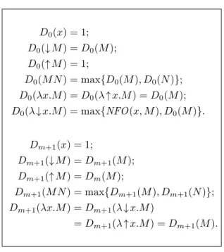
Proof. A formal proof could be given. We prefer, however, to give a more intuitive one here. Observe that:
D0(x) = 1; D0(↓ M ) = D0(M ); D0(↑ M ) = 1; D0(M N ) = max{D0(M ), D0(N )}; D0(λx.M ) = D0(λ ↑ x.M ) = D0(M ); D0(λ ↓ x.M ) = max{NFO (x, M ), D0(M )}. Dm+1(x) = 1; Dm+1(↓ M ) = Dm+1(M ); Dm+1(↑ M ) = Dm(M ); Dm+1(M N ) = max{Dm+1(M ), Dm+1(N )}; Dm+1(λx.M ) = Dm+1(λ ↓ x.M ) = Dm+1(λ ↑ x.M ) = Dm+1(M ).
Figure 10: Parametrised Duplicability Factor of Preterms: Equations.
• If Γ, x ` M or Γ, ↓ x ` M , then the variable x occurs free exactly once in M , in the first case outside the scope of any box, in the second case in the scope of exactly one inductive box. • If Γ, #x ` M , then x occurs free more than once in M , all the occurrences being outside the
scope of any box.
• The duplicability factor at level n of M is nothing more than the maximum, over all abstractions λ ↓ x.N at level n in M , of the number of free occurrences of x in N . Observe that by the well-formation rules in Figure 7, the variable x must be marked as #x or as ↓ x for any such N . If it is marked as ↓ x, however, it occurs once in N .
• Now, consider the substitution lemmas 9, 10, 11, 12, and 13. In all the five cases, one realises that:
1. for every n, Dn(M {x/N }) ≤ max{Dn(M ), Dn(N )}, because every abstraction occurring in M {x/N } also occurs in either M or N , and substitution is capture-avoiding.
2. If in the judgment Γ ` M {x/N } one gets as a result of the substitution lemma there is #y ∈ Γ, then NFO (y, M {x/N }) cannot be too big: there must be some z such that z is marked as #z in one (or both) of the provable judgments existing by hypothesis, but NFO (z, M ) + NFO (z, N ) majorises NFO (y, M {x/N }). Why? Simply because the only case in which NFO (y, M {x/N }) could potentially grow bigger is the one in which x is marked as #x in the judgment for M . In that case, however, the variables which are free in N are all linear (or marked as ↑ z or l z).
This concludes the proof.
Moreover, and this is the crucial point, Wn(M ) is guaranteed to strictly decrease whenever M →n•N :
Lemma 17. Suppose that M ∈ T`Λ4S
∞ and that M →n• N . Then Wn(M ) > Wn(N ). Moreover,
Wm(M ) = Wm(N ) whenever m < n.
Proof. We first of all need to prove the following variations on the substitution lemmas:
1. If Υ, x, #Θ, ↑ Ξ, l Ψ ` M and Π, #Θ, ↑ Ξ, l Ψ ` N , then for every n ≥ max{D0(M ), D0(N )} it holds that Wn
0(M {x/N }) ≤ W0n(M ) + W0n(N ).
2. If Υ, #Θ, #x, ↑ Ξ, l Ψ ` M and Φ, ↑ Ξ, l Ψ ` N , then for every n ≥ max{D0(M ), D0(N )} it holds that Wn
3. If Υ, #Θ, ↓ x, ↑ Ξ, l Ψ ` M and Φ, ↑ Ξ, l Ψ ` N , then for every n ≥ max{D0(M ), D0(N )} it holds that W0n(M {x/N }) ≤ W0n(M ) + n · W0n(N ).
4. If Υ, #Θ, ↑ Ξ, l Ψ, l x ` M and l Ψ ` N , then for every n ≥ max{D0(M ), D0(N )} it holds that W0n(M {x/N }) ≤ W0n(M ).
5. If Υ, #Θ, ↑ Ξ, ↑ x, l Ψ ` M and l Ξ, l Ψ ` N , then for every n ≥ max{D0(M ), D0(N )} it holds that W0n(M {x/N }) ≤ W0n(M ).
All the statements above can be proved, as usual, by induction on the (finite) number of inductive well-formation rules which are necessary to prove the judgment about M from something in C`Λ4S
∞(C`Λ4S∞). As an example, let us consider some inductive cases on Point 2., which is one of the
most interesting: • If M is proved well-formed by #Θ, ↑ Ξ, l Ψ, #x ` x (vd) then M {x/N } = N and W0n(M {x/N }) = W0n(N ) = 1 · W0n(N ) = NFO (x, M ) · W0n(N ) ≤ Wn 0(M ) + NFO (x, M ) · W n 0(N ). • If M is proved well-formed by Υ, #Θ, #x, ↑ Ξ, l Ψ ` L Π, #Θ, #x, ↑ Ξ, l Ψ ` P Υ, Π, #Θ, #x, ↑ Ξ, l Ψ ` LP (a) then M {x/N } = (L{x/N })(P {x/N }) and, by inductive hypothesis, we have
W0n(L{x/N }) ≤ W0n(L) + NFO (x, L) · W0n(N ); W0n(P {x/N }) ≤ W0n(P ) + NFO (x, P ) · W0n(N ). But then: W0n(M {x/N }) = W0n(L{x/N }) + W0n(P {x/N }) ≤ (W0n(L) + NFO (x, L) · W n 0(N )) + (W0n(P ) + NFO (x, P ) · W0n(N )) = (W0n(L) + W0n(P )) + (NFO (x, L) + NFO (x, P )) · W0n(N ) = W0n(M ) + NFO (x, M ) · W0n(N ). • If M is proved well-formed by Ξ, ↑ Ψ, l Φ ` M #Θ, #x, ↓ Ξ, ↑ Ψ, l Φ `↓ M (mi)
then x does not occur free in M and, as a consequence M {x/N } = M . The thesis easily follows. With the five lemmas above in our hands, it is possible to prove that if M 7→ N , then W0(M ) > W0(N ). Let’s proceed by cases depending on how M 7→ N is derived:
• If M = (λx.L)P , then Υ, x, #Θ, ↑ Ξ, l Ψ ` L and Π, #Θ, ↑ Ξ, l Ψ ` P . We can apply Point 1. (and Lemma 16) obtaining
W0(M ) = W D0(M ) 0 (M ) = W D0(M ) 0 (L) + W D0(M ) 0 (P ) + 1 > WD0(M ) 0 (L) + W D0(M ) 0 (P ) ≥ W D0(M ) 0 (L{x/P }) = WD0(M ) 0 (N ) ≥ W D0(N ) 0 (N ) = W0(N ). • If M = (λ ↓ x.L) ↓ P , then we can distinguish two sub-cases:
• If Υ, #x, #Θ, ↑ Ξ, l Ψ ` L and Φ, ↑ Ξ, l Ψ ` P , then we can apply Point 2. (and Lemma 16) obtaining W0(M ) = WD0(M ) 0 (M ) = WD0(M ) 0 (L) + D0(M ) · W D0(M ) 0 (P ) + 1 > WD0(M ) 0 (L) + D0(M ) · W D0(M ) 0 (P ) ≥ WD0(M ) 0 (L) + NFO (x, L) · W D0(M ) 0 (P ) ≥ WD0(M ) 0 (L{x/P }) = WD0(M ) 0 (N ) ≥ W D0(N ) 0 (N ) = W0(N ).
• If Υ, ↓ x, #Θ, ↑ Ξ, l Ψ ` L and Φ, ↑ Ξ, l Ψ ` P , then we can apply Point 3. (and Lemma 16) obtaining W0(M ) = W D0(M ) 0 (M ) = WD0(M ) 0 (L) + D0(M ) · W D0(M ) 0 (P ) + 1 > WD0(M ) 0 (L) + D0(M ) · W D0(M ) 0 (P ) ≥ WD0(M ) 0 (L{x/P }) = WD0(M ) 0 (N ) ≥ W D0(N ) 0 (N ) = W0(N ).
• If M = (λ ↑ x.L) ↑ P , then Υ, #Θ, ↑ x, ↑ Ξ, l Ψ ` L and ↑ Ξ, l Ψ ` P . We can apply Point 5. (and Lemma 16) obtaining W0(M ) = W D0(M ) 0 (M ) = W D0(M ) 0 (L) + 1 > WD0(M ) 0 (L) ≥ W D0(M ) 0 (L{x/P }) = WD0(M ) 0 (N ) ≥ W D0(N ) 0 (N ) = W0(N ).
Now, remember that M →n•N iff there are a n-context Cn• and two terms L and P such that
L 7→ P , M = Cn•[L], and N = Cn•[P ]. The thesis can be proved by induction on Cn•.
The Fundamental Lemma easily follows:
Proposition 3 (Fundamental Lemma). For every natural number n ∈ N, the relation →n• is
strongly normalising.
4.2
Normalisation and Confluence
The Fundamental Lemma has a number of interesting consequences, which make the dynamics of `Λ4S
∞ definitely better-behaved than that of `Λ∞. The first such result we give is a Weak-Normalisation Theorem:
Theorem 2 (Normalisation). For every term M ∈ T`Λ4S
∞ there is a normal form N ∈ T`Λ4S∞ such
that M ⇒ N .
Proof. This is an immediate consequence of the Fundamental Lemma: for every term M , first reduce (by →) all redexes at depth 0, obtaining N , and then normalise all the subterms of N at depth 1 (by ). Conclude by observing that reduction at higher depths does not influence lower depths.
The way the two modalities interact in `Λ4S
∞has effects which go beyond normalisation. More specifically, the two relations → and do not interfere like in `Λ∞, and as a consequence, we get a Confluence Theorem:
Theorem 3 (Strong Confluence). If M ∈ T`Λ4S
∞, M ⇒ N and M ⇒ L, then there is P ∈ `Λ
4S ∞ such that N ⇒ P and L ⇒ P .
The path to confluence requires some auxiliary lemmas:
Lemma 18. If Υ, #Θ, ↑ Ξ, l x, l Ψ ` M and l Ψ ` N , M ⇒ L, and N ⇒ P , then M {x/N } ⇒ L{x/P }.
Proof. This is a coinduction on M .
Lemma 19. If Υ, #Θ, ↑ Ξ, ↑ x, l Ψ ` M and l Ξ, l Ψ ` N , M L, and N ⇒ P , then M {x/N } L{x/P }.
Proof. This is again a coinduction on the structure of M , exploiting Lemma 18 Lemma 20 (Noninterference). If M ∈ T`Λ4S
∞, M →0•N and M L, then there is P ∈ `Λ
4S ∞such that N P and L →0•P .
Proof. By coinduction on the structure of M . Some interesting cases:
• If M = QR and Q →0•S, then N = SR. By definition, Q X and R Y , where L = XY .
By induction hypothesis, there is Z such that S Z and X →0•Z. The term we are looking
for, then, is just P = ZY . Indeed, N = SR ZY and, other other hand, L = XY →0•ZY .
• If M = (λ ↑ x.Q) ↑ R and N = Q{x/R}, then L is in the form (λ ↑ x.X) ↑ Y where Q X and R ⇒ Y , and then we can apply Lemma 18 obtaining that N P = X{x/Y }. On the other hand, L →0•P .
But there is even more: →0•and commute.
Lemma 21 (Postponement). If M ∈ T`Λ4S
∞, M N →0• L, then there is P ∈ `Λ
4S
∞ such that M →0•P L.
Proof. Again a coinduction on the structure of M . Some interesting cases:
• We can exclude the case in which M =↑ Q, because in that case also N would be a coinductive boxes, and coinductive boxes are →0•-normal forms.
• If M = (λ ↑ x.Q) ↑ R, N = (λ ↑ x.S) ↑ X (where Q S and R ⇒ X) and L = S{x/X}, then Lemma 18 ensures that P = Q{x/R} is such that P L.
One-step reduction is not in general confluent in infinitary λ-calculi. However, →0• indeed is:
Proposition 4. If M ∈ T`Λ4S ∞, M →
∗
0• N , and M →∗0• L, then there is P such that N →∗0• P
and L →∗0•P .
Proof. This can be proved with standard techniques, keeping in mind that in an inductive abstrac-tion λ ↓ x.M , the variable x occurs finitely many times in M .
The last two lemmas are of a techincal nature, but can be proved by relatively simple arguments: Lemma 22. Both and ⇒ are reflexive.
Proof. Easy.
Lemma 23. If M ∈ T`Λ4S
∞ and M →n•N (where n ≥ 1), then M N .
Proof. Easy, given Lemma 22
Proof of Theorem 3. We will show how to associate a term P = f (α) to any pair in the form α = (M ⇒ N, M ⇒ L) or in the form α = (M N, M L). The function f is defined by coinduction on the structure of the two proofs in α. This will be done in such a way that in the first case N ⇒ f (α) and L ⇒ f (α), while in the second case N f (α) and L f (α). If α is (M ⇒ N, M ⇒ L), then by definition, M →∗Q N and M →∗R L. Exploiting Lemma 23, Lemma 22, and Lemma 21, one obtains that there exist S and X such that M →∗0•S N and
M →∗
0•X L. By Proposition 4, one obtains that there is Y with S →∗0•Y and X →0•Y . By
repeated application of Lemma 20 and Lemma 22, one can conclude there are Z and W such that N →∗0• Z, Y Z, Y W and L →∗0• W . Now, let f (α) be just f (Y Z, Y W ).
If, on the other hand, α is (M N, M L), we can define f by induction on the proof of the two statements where, however, we are only interested in the last thunk of inductive rule instances. This is done in a natural way. As an example, if M is an application P Q, then clearly N is RS and L is XY , where P R, P X Q S, and Q Y ; moreover, f (α) is the term f (P R, P X)f (Q S, Q Y ). Notice how the function f is well defined, being a guarded recursive function on sets defined as greatest fixed points.
Confluence and Weak Normalisation together imply that normal forms are unique: Corollary 1 (Uniqueness of Normal Forms). Every term M ∈ T`Λ4S
∞ has a unique normal form.
Strangely enough, even if every term M has a normal form N , it is not guaranteed to reduce to it in every reduction order, simply because one can certainly choose to “skip” certain depths while normalising. In this sense, level-by-level sequences are normalising: they are not allowed to go to depth n > m if there is a redex at depth m.
4.3
Expressive Power
At this point, one may wonder whether `Λ4S∞ is well-behaved simply because its expressive power is simply too low. Although at present we are not able to characterise the class of functions which can be represented in it, we can already give some interesting observations on its expressive power.
First of all, let us observe that the inductive fragment of `Λ4S∞ (i.e. the subsystem obtained by dropping coinductive boxes) is complete for polynomial time computable functions on finite strings, although inputs need to be represented as Church numerals for the result to hold: this is a consequence of polytime completeness for SLL [21].
About the “coinductive” expressive power of `Λ4S
∞, we note that a form of guarded recursion can indeed be expressed, thanks to the very liberal exponential discipline of 4LL. Consider the term M = λ ↑ x.λy.λ ↑ z.y ↑ (xxz ↑ z) and define X to be M ↑ M . One can easily verify that for any (closed) term N , the term XN ↑ N reduces in three steps to N ↑ (XN ↑ N ). In other words, then, X is indeed a fixed point combinator which however requires the argument functional to be applied to it twice.
The two observations above, taken together, mean that `Λ4S
∞is, at least, capable of expressing all functions from (B∗)∞ to (B∗)∞ such that for each n, the string at position n in the output stream can be computed in polynomial time from the string at position n in the input stream. Whether one could go (substantially) beyond this is an interesting problem that we leave for further work. One cannot, however, go too far, since the 4LL exponential discipline imposes that all typable stream functions are causal, i.e., for each n, the value of the output at position n only depends on the input positions up to n, at least if one encodes streams as in Section 3.2.
5
Further Developments
We see this work only as a first step towards understanding how linear logic can be useful in taming the complexity of infinitary rewriting in the context of the λ-calculus. There are at least three different promising research directions that the results in this paper implicitly suggest. All of them are left for future work, and are outside the scope of this paper.
Semantics It would be interesting to generalise those semantic frameworks which work well for ordinary linear logic and λ-calculi to `Λ∞. One example is the so-called relational model of linear logic, in which formulas are interpreted as sets and morphisms are interpreted as binary relations. Noticeably, the exponential modality is interpreted by forming power multisets. Since the only kind of infinite regression we have in `Λ∞ is the one induced by coinductive boxes, it seems that the relation model should be adaptable to the calculus described here. Similarly, game semantics [2] and the geometry of interaction [14] seem to be well-suited to model infinitary rewriting.
Types The calculus `Λ∞is untyped. Incepting types into it would first of all be a way to ensure the absence of deadlocks (consider, as an example, the term (λ ↓ x.x)(↑ M )). The natural candidate for a framework in which to develop a theory of types for `Λ∞ is the one of recursive types, given their inherent relation with infinite computations. Another challenge could be adapting linear dependent types [7] to an infinitary setting.
Implicit Complexity One of the most interesting applications of the linearisation of Λ∞ as described here could come from implicit complexity, whose aim is characterising complexity classes by logical systems and programming languages without any reference to machine models nor to combinatorial concepts (e.g. polynomials). We think, in particular, that subsystems of `Λ∞ would be ideal candidates for characterising, e.g. type-2 polynomial time operators. This, however, would require a finer exponential discipline, e.g. an inductive-coinductive generalisation of the bounded exponential modality [12].
6
Related Work
Although this is arguably the first paper explicitly combining ideas coming from infinitary rewriting with resource-consciousness in the sense of linear logic, some works which are closely related to ours, but having different goals, have recently appeared.
First of all, one should mention Terui’s work on computational ludics [29]: there, designs (i.e. the ludics’ counterpart to proofs) are meant to both capture syntax (proofs) and semantics (functions), and are thus infinitary in nature. However, the overall objective in [29] is different from ours: while we want to stay as close as possible to the λ-calculus so as to inspire the design of techniques guaranteeing termination of programs dealing with infinite data structures, Terui’s aim is to better understand usual, finitary, computational complexity. Technically, the main difference is that we focus on the exponentials and let them be the core of our approach, while computational ludics is strongly based on focalisation: time passes whenever polarity changes.
Another closely related work is a recent one by Mazza [24], that shows how the ordinary, finitary, λ-calculus can be seen as the metric completion of a much weaker system, namely the affine λ-calculus. Again, the main commonalities with this paper are on the one hand the presence of infinite terms, and on the other a common technical background, namely that of linear logic. Again, the emphasis is different: we, following [19], somehow aim at going beyond finitary λ-calculus, while Mazza’s focus is on the subrecursive, finite world: he is not even concerned with reduction of infinite length.
If one forgets about infinitary rewriting, linear logic has already been shown to be a formidable tool to support the process of isolating classes of λ-terms having good, quantitative normalisation properties. One can, for example, cite the work by Baillot and Terui [3] or the one by Gaboardi and Ronchi here [11]. This paper can be seen as a natural step towards transferring these techniques to the realm of infinitary rewriting.
Finally, among the many works on type-theoretical approaches to termination and productivity, the closest to ours is certainly the recent contribution by Cave et al. [6]: our treatment of the coinductive modality is very reminiscent to their way of handling LTL operators.