HAL Id: hal-00730995
https://hal.archives-ouvertes.fr/hal-00730995
Preprint submitted on 11 Sep 2012
HAL is a multi-disciplinary open access archive for the deposit and dissemination of sci-entific research documents, whether they are pub-lished or not. The documents may come from teaching and research institutions in France or abroad, or from public or private research centers.
L’archive ouverte pluridisciplinaire HAL, est destinée au dépôt et à la diffusion de documents scientifiques de niveau recherche, publiés ou non, émanant des établissements d’enseignement et de recherche français ou étrangers, des laboratoires publics ou privés.
Technical Report: CSVM Ecosystem
Frédéric Rodriguez
To cite this version:
Technical Report: CSVM Ecosystem
Using CSVM format in various scientific fields.
Frédéric Rodriguez
a,b,* aCNRS, Laboratoire de Synthèse et Physico-Chimie de Molécules d’Intérêt Biologique, LSPCMIB, UMR-5068, 118 Route de Narbonne, F-31062 Toulouse Cedex 9, France.
b
Université de Toulouse, UPS, Laboratoire de Synthèse et Physico-Chimie de Molécules d’Intérêt Biologique, LSPCMIB, 118 route de Narbonne, F-31062 Toulouse Cedex 9, France.
Abstract
The CSVM format is derived from CSV format and allows the storage of tabular like data with a limited but extensible amount of metadata. This approach could help computer scientists because all information needed to uses subsequently the data is included in the CSVM file and is particularly well suited for handling RAW data in a lot of scientific fields and to be used as a canonical format. The use of CSVM has shown that it greatly facilitates: the data management independently of using databases; the data exchange; the integration of RAW data in dataflows or calculation pipes; the search for best practices in RAW data management. The efficiency of this format is closely related to its plasticity: a generic frame is given for all kind of data and the CSVM parsers don’t make any interpretation of data types. This task is done by the application layer, so it is possible to use same format and same parser codes for a lot of purposes. In this document some implementation of CSVM format for ten years and in different laboratories are presented. Some programming examples are also shown: a Python toolkit for using the format, manipulating and querying is available. A first specification of this format (CSVM-1) is now defined, as well as some derivatives such as CSVM dictionaries used for data interchange. CSVM is an Open Format and could be used as a support for Open Data and long term conservation of RAW or unpublished data.
Keywords
RAW Data, Tabular Data, CSV, Metadata, Data exchange, Dataflow, Canonical format, Python language, web-publishing framework, Chemistry, Bioinformatics, Enzyme science, Structural Biology, Environmental Sciences, Open Format, Open Data.
* Corresponding authors.
CNRS, Laboratoire de Synthèse et Physico-Chimie de Molécules d’Intérêt Biologique, LSPCMIB, UMR-5068, 118 Route de Narbonne, F-31062 Toulouse Cedex 9, France.
Tel.: þ33 (0) 5 61556486; fax: þ33 (0) 5 61556011.
1. The basics: table, file, annotations and a programming sample
This CSVM sample is relative to the field of medicinal chemistry, courtesy from Pascal Hoffmann and coll 1 2
. This is the case of a collection of 80 molecular files (af01.mdl, af02.mdl, …, af80.mdl) in a directory. Each file stores the molecular 2D coordinates (formula) for a given compound, using a given format (here MDL Molfile format 3).
Figure 1. –A view 4 of the molecule’s collection.
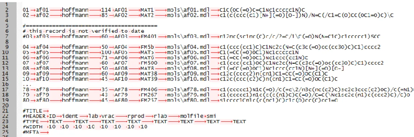
We wanted to store a table of these molecules, including the molecule’s number (ID), an identifier (ident), the chemist related to the compound synthesis (lab), an amount (vrac) available of the compound, another compound identifier (rprod), the related laboratory notebook identifier (rlab), the molecular file itself (molfile) including a relative and the compound formula (smi) written in another format (here SMILES 5 chemical format) and included in a cell of the table:
Figure 2. –A view of the collection written in a table, only rows [1..10] and [78..80] are shown.
ID ident lab vrac rprod rlab molfile smi
1 af01 hoffmann 114 AF01 MAT1 mols\af01.mdl C1C(OC(=O)C=C1Nc1ccccc1N)C
2 af02 hoffmann 85 AF02 MAT2 mols\af02.mdl c1(c(ccc(c1)[N+](=O)[O-])N)/N=C(/C1=C(O)CC(OC1=O)C)\C 3 af03 hoffmann 60 AF03 FM401 mols\af03.mdl n12nc(sc1nc(C)c/c/2=C/1\C(=O)N(N=C1C)c1ccccc1)SCC 4 af04 hoffmann 50 AF04 FM5b mols\af04.mdl c1(ccc(cc1)C)C1Nc2c(N=C(c3c(=O)oc(cc3O)C)C1)cccc2 5 af05 hoffmann 100 AF05 MAT5 mols\af05.mdl C1(=CC(=O)OC1)Nc1ccccc1N
6 af06 hoffmann 71 AF06 MAT6 mols\af06.mdl C1(=CC(=O)OC1)Nc1ccc(cc1N)C
7 af07 hoffmann 60 AF07 FM500 mols\af07.mdl c1(ccc(cc1)OC)C1Nc2c(N=C(c3c(=O)oc(cc3O)C)C1)cccc2 8 af08 hoffmann 50 AF08 MAT8 mols\af08.mdl C1(=CC(=O)OC1)Nc1ccc(cc1N)[N+](=O)[O-]
9 af09 hoffmann 60 AF09 MAT38 mols\af09.mdl c12c(cccc2)n(cn1)C1=CC(=O)OC(C1)C 10 af10 hoffmann 45 AF10 MAT39 mols\af10.mdl c12c(ccc(c2)C)n(cn1)C1=CC(=O)OC(C1)C . . .
1
L. Hammal, S. Bouzroura, C. André, B. Nedjar-Kolli, P. Hoffmann (2007) Versatile Cyclization of Aminoanilino Lactones: Access to Benzotriazoles and Condensed Benzodiazepin-2-thione. Synthetic Commun., 37:3, 501-511.
2
M .Fodili, M. Amari, B. Nedjar-Kolli, B. Garrigues, C. Lherbet, P. Hoffmann (2009) Synthesis of Imidazoles from Ketimines Using Tosylmethyl Isocyanide (TosMIC) Catalyzed by Bismuth Triflate. Lett. Org. Chem., 6, 354-358.
3
Chemical table file [Wikipedia] - http://en.wikipedia.org/wiki/Chemical_table_file
4
78 af78 hoffmann 35 AF78 FM406 mols\af78.mdl c1(ccccc1)N1C(=O)/C(=c\2/n3c(nc(c2)C)sc2c3ccc(c2)OC)/C(=N1)C 79 af79 hoffmann 43 AF79 FM267 mols\af79.mdl c1(ccccc1)n1c(c(c(n1)C)C(=O)/C=C(\Nc1sc2c(n1)c(ccc2)C)/C)O 80 af80 hoffmann 45 AF80 FM257 mols\af80.mdl s1cccc1Cn1c(c(nc1)C)c1c(O)cc(C)oc1=O
Then we wanted to write the table: i) as a CSV derived file for data and ii) with a block for metadata:
Figure 3. –The corresponding CSVM file (rows [1..10] and [78..80]).
This is what we call a CSVM file (CSV with Metadata). In this case the field separator is a TAB (red arrows) but the CSVM specification allows any character. The data block is the same than shown in Figure 2 but it is followed by rows beginning with # character and defining a metadata block.
Using flat CSVM files (CSVM-1 specification) the # rows are considered as metadata rows if the # is immediately followed by a known keyword (TITLE, HEADER, TYPE, WIDTH, META). If the keyword is not recognized by the CSVM parser, the row is not processed.
This is also possible to use this property in order to extinct some data rows in the CSVM without deleting them; and to annotate the file adding rows for remarks. The following CSVM illustrates these two cases outside the metadata block (rows 5, 6, 7). The blank lines are not taken in account by the CSVM parser, so they could be used to make the table more readable for humans. As a result, in Figure 4 the compound with ID=3 will not be included in data structure stored in computer’s memory.
Figure 4. –A tagged (remarks) CSVM file.
The metadata block is used to embed the minimal canonical information about the table:
The #TITLE row is for information (one ASCII line) about the table.
The #HEADER row stores for column titles.
The #TYPE row stores for the data types for columns. CSVM lets you define your data types, only fuzzy and very minimal data types are provided: TEXT (textual data), NUMERIC (columns of integer or float values), BOOLEAN (0/1, Y/N, Yes/No you can define your own code).
The #WIDTH row is used to store a value significant of column’s width.
The CSVM parser don’t use the information stored in metadata block: all the information is read as strings and returned as a data structure depending on the programming language used.
Metadata is not interpreted at the parser level and it is a choice. Using this approach makes it possible to add all data types for #TYPE keywords, this is the reason of the reduced number of predefined types in CSVM specification. The data type recognition is done only when the data structure is available in memory: this step is uncoupled from the parser step. A side result is that the same parser can be used for all data types.
In the case of Python language, a Class (a csvm_ptr object) is returned with some methods (i.e. csvm_ptr_dump for display the data structure on standard output). The following code (Code 1) shows the contents of the corresponding data structure. These lines are extracted from a Python toolkit (Pybuild) that support CSVM files.
Code 1. – Beginning of Python CSVM Class code. class csvm_ptr:
"""
Follows CSVM specs (v:1.x) for contents of data structure. Standard column types are NUMERIC,TEXT,DATE,BOOLEAN. Some of us, use also INTEGER, FLOAT for numeric types. Some of us, use also NODE, LINK, IMAGE for web data embedded in CSVM files. WIDTHs (10,50 if not set) are for Javascript tables and can be omitted.
*** 1.01/080304/fred """
def __init__(self):
self.SOURCE = "" # path/file name of readed CSVM file
self.CSV = "" # CSVM or CSV depending of file contents
self.TITLE_N = 0 #Titles of CSVM file (let for future, only one string used today)
self.TITLE = "" # Title of CSVM file
self.HEADER_N = 0 # Number of data columns titles
self.HEADER = [] # List of data column titles
self.TYPE_N = 0 # Number of data columns types (= self.HEADER_N)
self.TYPE = [] # List of data column types
self.WIDTH_N = 0 # Number of data columns widths (= self.HEADER_N)
self.WIDTH = [] # List of data column widths
self.DATA_R = 0 # Number of data rows
self.DATA_C = 0 # Number of data columns (= self.HEADER_N)
self.DATA = [] # String matrix containing data
self.META = "" # Meta string
The following Python code (Code 2) shows how 1) to load a CSVM file (using the TAB “\t” as delimiter) with the function csvm_ptr_read_extended_csvm, 2) to display the Class and 3) to free the memory.
Code 2. – Loading and printing a CSVM file using Pybuild toolkit. print "=> A new blank CSVM object"
c = csvm_ptr()
print "=> Populates it with a CSVM file ... "
c = csvm_ptr_read_extended_csvm(c, file_cleanpath("test/hoffmann.csvm"), "\t") print "=> data dump ... "
c.csvm_ptr_dump(0,0)
print "=> Clear CSVM object" c.csvm_ptr_clear()
The corresponding output is shown in Figure 5, the result of csvm_ptr_dump method shows the metadata block (pink text, the order of metadata rows is #WDITH, #TEXT, #HEADER) followed by data rows (all cells are surrounded by brackets). Please notice that the previous annotated CSVM file is used: the row with [03] value in first column {number} is missing.
2. Advanced: combining with databases
CSVM is obviously not a substitute for databases, but it is possible to use a CSVM table for storing simple database schema and database tables. The following sample shows this kind of approach in the case of a chemical inventory. These files were generated after analysis (SQL requests) of a relational database system (Hughes Technologies mQSL) and prior to be converted and injected in another RDBMS (MySQL or PostgreSQL).
2.1. Database tables and schema – Chemical inventory
A simple chemical database of two tables and a relation between the column of indice=3 (from 0 to n-1) in table ‘assoc’ to column of indice=0 in table ‘user’. Note that the schema contains heterogeneous data in columns (data from keyword TABLES, or FOREIGN) so all columns titles are set to the same word ‘DATA’, courtesy from Anne Laure Leomant 6
and Nathalie Gouardères.
Figure 6. – Example of database schema encoded in a CSVM file.
DB 192.168.10.17 anonymous - Chemb TABLE user chemb\user.csvm 0 - TABLE assoc chemb\assoc.csvm 0 - FOREIGN assoc 3 user 0
#TITLE Database import schema
#HEADER KEYWORD DATA DATA DATA DATA #TYPE TEXT TEXT TEXT TEXT TEXT #WIDTH 10 10 10 10 10 #META april/25/2008 15:42:45
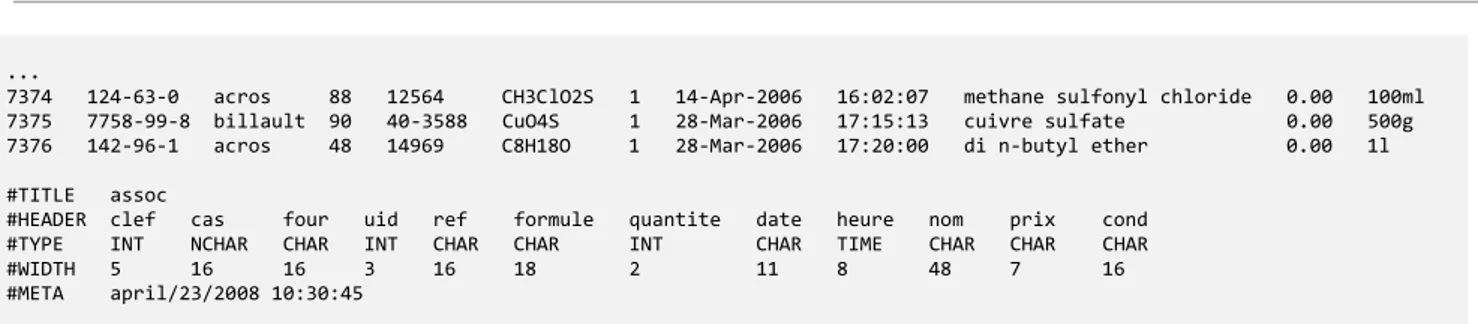
The database tables are a particular case of CSVM file. Database systems have specific data types (i.e. REAL, INTEGER, SMALLINT …) depending on the records used in tables that are more precise than the generic CSVM type (NUMERIC in this case). But the CSVM approach allows the use of database types in metadata #TYPE row. Also in row #WIDTH it is possible to store the dimension of database fields when it is needed by database type. The following example shows the last 3 lines of CSVM file assoc.csvm corresponding to the ‘assoc’ table included in of the previous schema:
Figure 7. – Example of a database table encoded in a CSVM file.
...
7374 124-63-0 acros 88 12564 CH3ClO2S 1 14-Apr-2006 16:02:07 methane sulfonyl chloride 0.00 100ml 7375 7758-99-8 billault 90 40-3588 CuO4S 1 28-Mar-2006 17:15:13 cuivre sulfate 0.00 500g 7376 142-96-1 acros 48 14969 C8H18O 1 28-Mar-2006 17:20:00 di n-butyl ether 0.00 1l
#TITLE assoc
#HEADER clef cas four uid ref formule quantite date heure nom prix cond #TYPE INT NCHAR CHAR INT CHAR CHAR INT CHAR TIME CHAR CHAR CHAR #WIDTH 5 16 16 3 16 18 2 11 8 48 7 16 #META april/23/2008 10:30:45
Notice that other information on databases (i.e. data types for descriptions and conversions) could be also encoded in CSVM files.
So CSVM, even if it is primarily conceived for handling RAW data is also usable to get a ‘flat’ view of simple database systems. It could be used as a canonical format to do a lot of transformation between databases, without any modification of CSVM parsers.
3. Indexes, collection of files, documents …
Initially CSVM was used primarily for indexing purposes: file’s catalog (filenames/paths and some metadata about the files) rather than as a substitute for spreadsheets tables. The following figure shows this kind of use: the result for a recursive directory list.
Figure 8. – Example of using a CSVM table for a file catalog (this output is a dump of a CSVM Python class).
DUMP: CSVM info { SOURCE CSV CSVM META [] TITLE_N 1 TITLE HEADER_N 3 TYPE_N 3 WIDTH_N 3 0 50 TEXT {DIR} 1 50 TEXT {FILE} 2 50 TEXT {-} DATA_R 118 DATA_C 3 118 3 0 [c:\Python26\Lib\site-packages\build][args.py][18:jun:2009] 1 [c:\Python26\Lib\site-packages\build][date.py][19:oct:2006] 2 [c:\Python26\Lib\site-packages\build][dir.py][06:may:2010] ... 115 [c:\Python26\Lib\site-packages\build\_depot\numerix\_dist][__init__.py][16:apr:2008] 116 [c:\Python26\Lib\site-packages\build\_struct][strpdb.py][26:mar:2007] 117 [c:\Python26\Lib\site-packages\build\_struct][__init__.py][31:oct:2006] } done
Notice that the last column is filled by the date of creation of files, but the column name is pending (the #HEADER value is a blank) before saving data in a CSVM file. This is a very interesting feature of CSVM approach related to RAW data: in some circumstances the name of a column is not yet defined but the data must be stored anyway.
3.1. Software pipes – Molecular calculations
CSVM can be useful for launching calculations, you can store in the CSVM the operations to do, including launching external programs, store intermediate results (or index filenames) and complete or add columns from step to steps. Eventually a software component using a CSVM parser can generate from these tables, information (files, parameters) needed by job schedulers/batch processors.
Very often calculations are applied to data files, so this is a particular case of indexing. The interest of CSVM space is that all steps (defining files, parameters, results) could be made easily and in the same data format (ready for use by spreadsheets or scientific data analysis and graphic software).
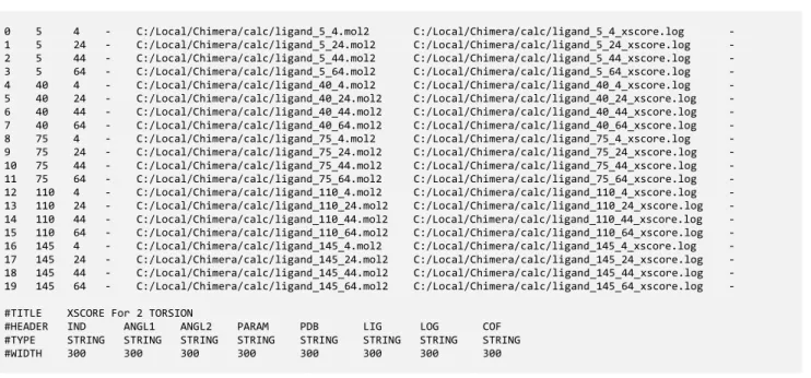
In the next section, a complete example will be shown (case of Enzyme kinetics). Here a simpler sample issued from [structural biology/rational drug design] science is given. The data shown is a CSVM file, used by a software component added to UCSF Chimera 78 software and used to launch X-Score 910 calculations inside the interface, courtesy from Mansi Trivedi 11.
Each calculation uses a ligand and a protein. For a given ligand, one or two torsion angles were selected using the Chimera GUI and different files (‘PARAM‘ column) corresponding to different angular values
7
UCSF Chimera - http://www.cgl.ucsf.edu/chimera/
8
UCSF Chimera--a visualization system for exploratory research and analysis. E.F. Pettersen, T.D. Goddard, C.C. Huang, G.S. Couch, D.M. Greenblatt, E.C. Meng, T.E. Ferrin. J Comput. Chem. (2004) 25:13, 1605-1612.
9
Renxiao Wang – http://sw16.im.med.umich.edu/software/xtool/
10
R. Wang, Y. Lu, S. Wang. Comparative Evaluation of 11 Scoring Functions for Molecular Docking. J. Med. Chem. (2003) 46:12, 2287-2303.
11
M. Trivedi – In silico approach to study protein-ligand binding affinity. Rapport M2P Bioinformatique, Université Paul Sabatier (2009).
(’ANG1’ and ’ANG2’ columns) were generated. For calculation the corresponding log files were added (’LOG’ column) in the CSVM table.
Figure 9. – Calculations driven by a CSVM table.
0 5 4 - C:/Local/Chimera/calc/ligand_5_4.mol2 C:/Local/Chimera/calc/ligand_5_4_xscore.log - 1 5 24 - C:/Local/Chimera/calc/ligand_5_24.mol2 C:/Local/Chimera/calc/ligand_5_24_xscore.log - 2 5 44 - C:/Local/Chimera/calc/ligand_5_44.mol2 C:/Local/Chimera/calc/ligand_5_44_xscore.log - 3 5 64 - C:/Local/Chimera/calc/ligand_5_64.mol2 C:/Local/Chimera/calc/ligand_5_64_xscore.log - 4 40 4 - C:/Local/Chimera/calc/ligand_40_4.mol2 C:/Local/Chimera/calc/ligand_40_4_xscore.log - 5 40 24 - C:/Local/Chimera/calc/ligand_40_24.mol2 C:/Local/Chimera/calc/ligand_40_24_xscore.log - 6 40 44 - C:/Local/Chimera/calc/ligand_40_44.mol2 C:/Local/Chimera/calc/ligand_40_44_xscore.log - 7 40 64 - C:/Local/Chimera/calc/ligand_40_64.mol2 C:/Local/Chimera/calc/ligand_40_64_xscore.log - 8 75 4 - C:/Local/Chimera/calc/ligand_75_4.mol2 C:/Local/Chimera/calc/ligand_75_4_xscore.log - 9 75 24 - C:/Local/Chimera/calc/ligand_75_24.mol2 C:/Local/Chimera/calc/ligand_75_24_xscore.log - 10 75 44 - C:/Local/Chimera/calc/ligand_75_44.mol2 C:/Local/Chimera/calc/ligand_75_44_xscore.log - 11 75 64 - C:/Local/Chimera/calc/ligand_75_64.mol2 C:/Local/Chimera/calc/ligand_75_64_xscore.log - 12 110 4 - C:/Local/Chimera/calc/ligand_110_4.mol2 C:/Local/Chimera/calc/ligand_110_4_xscore.log - 13 110 24 - C:/Local/Chimera/calc/ligand_110_24.mol2 C:/Local/Chimera/calc/ligand_110_24_xscore.log - 14 110 44 - C:/Local/Chimera/calc/ligand_110_44.mol2 C:/Local/Chimera/calc/ligand_110_44_xscore.log - 15 110 64 - C:/Local/Chimera/calc/ligand_110_64.mol2 C:/Local/Chimera/calc/ligand_110_64_xscore.log - 16 145 4 - C:/Local/Chimera/calc/ligand_145_4.mol2 C:/Local/Chimera/calc/ligand_145_4_xscore.log - 17 145 24 - C:/Local/Chimera/calc/ligand_145_24.mol2 C:/Local/Chimera/calc/ligand_145_24_xscore.log - 18 145 44 - C:/Local/Chimera/calc/ligand_145_44.mol2 C:/Local/Chimera/calc/ligand_145_44_xscore.log - 19 145 64 - C:/Local/Chimera/calc/ligand_145_64.mol2 C:/Local/Chimera/calc/ligand_145_64_xscore.log -
#TITLE XSCORE For 2 TORSION
#HEADER IND ANGL1 ANGL2 PARAM PDB LIG LOG COF #TYPE STRING STRING STRING STRING STRING STRING STRING STRING #WIDTH 300 300 300 300 300 300 300 300
After calculation, the log files generated by X-SCORE were parsed, converted in CSVM tables, and the tables were indexed (extraction of score values). Then, the score values were aggregated with the upper table (addition of columns). All the process is driven by the table of Figure 9 that contains all information needed for calculation and collection of results. In this case the first column (‘IND’) is used for store indices of rows but it can be used in key/values scheme, as it was done in the following sample:
Figure 10. – Calculation and parameters driven by a CSVM table, columns PHI and PSI are used for angle values.
The first column labeled ‘KW’ stores keyword that drives contents of next columns, and the last column (‘SCORE’) is present and ready to store score values. The CSVM file is used to store parameters/results of calculations (rows 7-25) as well as configuration options of X-SCORE (rows 2-6). This case shows that in the same format space we can store configurations, parameters, results …
4. From indexes to collections: files, information and dataflows
The concept was then used for indexes and for tabular data in the same or different collections. For a same catalog, the two next samples show differences (files vs. tables) on indexed contents: i) the case of a publishing chain (for standard files) and ii) the case of a collection of sparse environmental data (for CSVM files). These two examples are issued from scientific works in the field of environmental sciences, but making collections of RAW/processed objects is a general problem in all sciences.
4.1. A publishing chain
The process starts from a set of documents (books, articles, reports, various documents) about a particular place (Malause) known as a sedimentation zone in a river (Garonne, France). Courtesy from Philippe Vervier, Sarah Gimet 12 and Gerome Beyries 13.
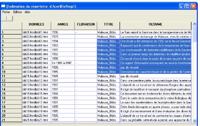
This grey information (because all documents are not indexed in bibliographic systems) was digitized (PDF to ASCII text) and contents were extracted (text filters), normalized and saved in Open Office documents (using a common template). This new collection of documents was then used as a primary data source by software components: converted in XML (XML DocBook 14), HTML 15 and analyzed using a custom XML parser. Pertinent fields of information found in documents (year, title, abstract …) were extracted and saved in a CSVM file. Courtesy from Jean-Olivier Butron 16.
The following figure shows a Perl CSVM parser that displays CSVM data in a grid widget. The column ‘DONNEES’ contains links to the corresponding HTML documents (URL|Name of URL), ‘ANNEE’ stands for year, ‘TITLE’ for title and ‘RESUME’ for abstract.
Figure 11. –A simple viewer (wxGrid widget 17) parsing a CSVM file (a collection of documents).
12
M. Gerino & coll. Bilan et dynamique de la matière organique et des contaminants au sein d’une discontinuité ex de la retenue de Malause. Restitution des travaux scientifiques du projet de recherche ECOBAG P2 (2006).
13
G. Beyries. Composants logiciels génériques pour les collections de données. Mémoire ingénieur Ecole des Techniques du Génie Logiciel (2004).
14
XML DocBook - http://www.docbook.org/
15
Norman Walsh style sheets - http://nwalsh.com/
16
F. Rodriguez, G. Beyries, J.O. Butron, C. Blonski. Maîtriser l’information chimique au quotidien: méthodes et composants logiciels à l’interface chimiebiologie. JECB21, Toulouse (2005).
17
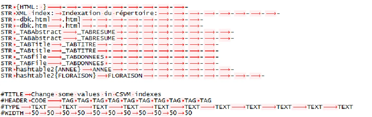
In this case the CSVM file corresponds to the index of this collection and embeds information extracted from documents. At the CSVM level: this is data; at indexed files (XML files converted in HTML files) level: this is metadata. All the different tasks were processed automatically without data input ‘at hand’ by an operator. A lot of conversion between files (Raw text, HTML, XML, XML-Docbook, HTML) were also configured and driven by CSVM files. The following figure shows a CSVM file used to drive changes in the CSVM index itself (each row is a filter applied to the index).
Figure 12. – Some rows of a CSVM files filled with rules for a text filter.
The first column is used to store the type of filter using a keyword. The keyword STR is used to specify a string replacement of the value stored in second column by the value stored by the third column. More complex filters that ‘STR’ exist and need to use fully the 10 columns. Then the CSVM index was integrated with a JavaScript framework in order to provide a view of the collection dedicated to end users. Buttons at the top of dynamic table are used to sort data of CSVM index by a given column.
Figure 13. – Same data (as shown in Figure 10) parsed using a JavaScript list component and displayed as item list (bibliographic style) rather than columns. Data are sorted by year (ANNEE) and displayed in the order (ANNEE, DONNEES, FLORAISON, TITRE, RESUME).
When the publishing chain works, all to do is to write the CSVM file and to process the chain. Edition of the CSVM index can be done, manually (text editor), using a GUI, automatically by an indexer component). In this case the documents were stored in HTML (after processing) or native (hyperlink to the corresponding file or image) formats.
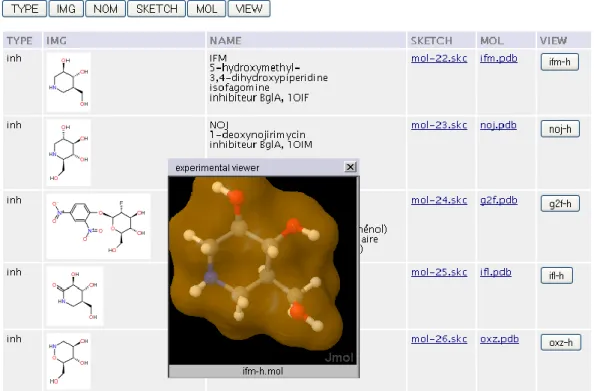
The following figure shows final results for this kind of publishing chain: 14-A) the case of small organic molecules (ligands, inhibitors) interacting with some enzymes (GlcCerase, beta-glucosidase) and 14-B) the case of enzymes itself (HAT).
Figure 14-A. – Chemical collection of ligands taken from the Protein Data Bank 18.
Figure 14-B. – Collection of macro-molecules (enzymes) structures taken from the Protein Data Bank.
18
Courtesy from Marjorie Catala 19 ; Casimir Blonski, Christian Lherbet and Cecile Baudoin-Dehoux 2021 .
The previous figure (14-A) shows the case of a chemical collection (small organic molecules). The collection mixes images (‘IMG’ column), some information (TYPE, NOM), 2D (SKETCH) and native 3D (MOL) structures and action buttons (VIEW) launching an external viewer 22 embedded (HTML layer) in a floating window. In the case of Figure 14-B, the interface of the molecular collection (macromolecules) is multimodal and could launch local/hyperlinks (‘FILE’/’LINK’ columns), PyMol 23 generated images (‘IMAGE’) of structure, a viewer (‘JMOL’) as other information.
From a CSVM point of view (RAW data) the samples of Figure 13-14-15 are of the same complexity despite the kind of objects displayed. All is taken in account by a different JavaScript framework: the CSVM data were converted in JavaScript tables and were processed by dedicated JavaScript components. The Following Code shows the contents of this kind of JavaScript table and the first row for the molecular structure displayed in the case of Figure 14-A:
Code 3. – A JavaScript table descending from a CSVM file.
// GXMLPARSER interface, download these data before, // and use GXMLDISPLAY for use whith browsers
function jmol(mol,button)
{ var src = "<INPUT onclick=" + '"' + "loadwindow('jmol.html',250,287,'" + mol + "');" + '"' + "type=button value='" + button + "'>";
return(src); }
var flags_array = new Array ("TYPE", "SECTOR", "IMG", "NAME", "SKETCH", "MOL", "VIEW"); var flags_n=7;
var getf_array = new Array ("TYPE", "IMG", "NAME", "SKETCH", "MOL", "VIEW"); var getf_n=6;
var data_c=7;
var data_array = new Array();
var data_r=0;
. . .
data_array[data_r++] = new Array ("inh", "glccerase", "<IMG SRC='sketch/mol-22.png'>", "IFM<br>5-hydroxymethyl-3,4-dihydroxypiperidine<br>isofagomine<br>inhibiteur BglA, 1OIF", "<A HREF='sketch/mol-22.skc'>mol-22.skc</A>", "<A HREF='lig/ifm.pdb'>ifm.pdb</A>",
jmol('ifm-h.mol','ifm-h')); . . .
It is easy to transform a CSVM file in another tabular data (i.e. JavaScript, CSV, XML tables) format because all that is needed to do the transformation is embedded in the CSVM file itself.
The corresponding index CSVM files can be edited manually by users (as they were using spreadsheet tables) or automatically generated, but the CSVM mechanism has the advantage of providing a lot of features for further processing and transformations.
19
M. Catala - Etude structurale et arrimage moléculaire (Docking) in silico de prodrogues dans la ß-glucocérébrosidase. Rapport M1BBT (2006) Université Paul Sabatier.
20
S. Gau, F. Rodriguez, C. Lherbet, C. Menendez, M. Baltas. Approches interdisciplinaires pour la conception rationnelle d’inhibiteurs. RECOB 13, Aussois (2010).
21
New potent bisubstrate inhibitors of histone acetyltransferase p300: design, synthesis and biological evaluation. F.H.A. Kwie, M. Briet, D. Soupaya, P. Hoffmann, M. Maturano, F. Rodriguez, C. Blonski, C. Lherbet, C. Baudoin-Dehoux. Chem Biol
Drug Des. (2011) 77:1, 86-92. 22
4.2. Environmental tabular data
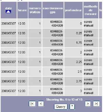
This sample shows a way to dig inside files when the indexed files are also CSVM files. An index was also created but each entry was linked to a CSVM file rather than a text document (Open Office, XML, HTML, PDF …) or a data source (data file, image, hyperlinks).
In this case, the CSVM data (table of measurements, not index) were written manually using a standard spreadsheet. Courtesy from Magali Gerino, Maya Lauriol, Sabine Sauvage 24 and Gerome Beyries 25.
As in previous case, end users can download corresponding CSVM files using an hyperlink in index display, but also they can view (after another CSVM conversion in JavaScript tables of each leaf files) directly inside these files using another JavaScript framework 26, as shown by the following figure:
Figure 15. – A dynamic view of a CSVM file after its conversion (JavaScript table, columns at right not shown).
In this table the #WIDTH information is used for column’s widths and #TYPE values are injected as column’s names in the JavaScript tables.
CSVM can be used as well as for index and for tables. This approach has a great potential for complex processing of files because one parser and one format are used independently of tabular objects and information.
24
M. Gerino & coll. Bilan et dynamique de la matière organique et des contaminants au sein d’une discontinuité ex de la retenue de Malause. Restitution des travaux scientifiques du projet de recherche ECOBAG P2 (2006).
25
G. Beyries, F. Rodriguez. Quels outils informatiques pour les collections de données ? Restitution du Programme ECOBAG P1, Agen (2004).
26
A modified version of Dieter Bunger’s (http://www.infovation.de) Cross Browser Dynamic HTML Tables code -
4.3. Working with RAW tables
Typically a case encountered in collaborative projects, in which the aggregation of RAW data from different scientific fields (and different data types by definition) is expected. The CSVM concept makes easy to compute intersection or union of tables which could be often useful. These operations are possible even if the tables cover the 1) same, 2) a common core, and 3) different sets of data. In Python CSVM toolkit the union or intersection of CSVM tables use csvm_ptr() objects :
print "\n*** Test completely different CSVM files" c1 = csvm_ptr()
c1 = csvm_ptr_read_extended_csvm(c1,"test/test1.csvm","\t")
c2 = csvm_ptr()
c2 = csvm_ptr_read_extended_csvm(c2,"test/test2.csvm","\t")
The two CSVM files were loaded in two csvm_ptr() objects c1 and c2, now the intersection of the two tables can take place, the result is a new csvm_ptr() named r :
print "=> Compute INTERSECTION" r = csvm_ptr_intersect(c1, c2) if (r != None):
r.csvm_ptr_dump(0,0)
r.csvm_ptr_clear() else:
print "No data found"
The union of tables is coded as same, and after operation all data structures are destroyed 27.
print "\n=> compute UNION" r = csvm_ptr_union(c1, c2) r.csvm_ptr_dump(0,0)
r.csvm_ptr_clear() c1.csvm_ptr_clear() c2.csvm_ptr_clear()
print "\n*** Test csvmutil done."
Notice that after (and sometimes before) union of tables with different (names and types) columns, the RAW data can be sparse, typically a big number of columns, without data for some (or nearly all) rows. If same columns are found in c1 and c2 tables, the union mechanism preserves data because data blocks (rows) are added successively and not interleaved.
For an attentive reader, just remark something on Figure 13: the presence of a file named pinguicula_vulgaris. This file contains information about a carnivorous plant (butterworts) which seems not to be included in the same category than the others (bibliographic digests about stations around Malause: malause_biblio): this is the result of union of tables from different CSVM files.
In the case of pinguicula a year was not extracted or assigned from data file, and the resulting cell in final CSVM file is marked by the empty character (‘-‘ in this case), the CSVM puinguicula branch has not this column. The last column is an excerpt of the [abstract/beginning of the text] found in files. The pingucula type CSVM files have not this kind f information. But, the text recognized as title (not filename) inside the document was assigned to a particular column. This column was later and prior to union of tables set as equivalent to the ‘RESUME’ column of malause_biblio branch. So this column is filled in the resulting CSVM file that was processed in the dataflow. Another mechanism was also used: adding 28 a column ‘FLORAISON’
(flowering date) not found in the malause_biblio branch and obviously found in pinguicula branch.
This shows how it is possible to manipulate and aggregate RAW data easily in CSVM space without any data modeling
5. From collections to calculations: the case of time series
The case of enzyme kinetics is interesting because the CSVM format can be used in different ways: to store i) data (time series); ii) parameters for calculation (modeling, curve fitting); iii) results (best fit, residuals, parameter’s values) and sometimes iv) the model itself. These steps can be found in a lot of other scientific fields (i.e. Physics, Chemistry) in which modeling is used as a core technique.
Enzyme kinetics measurements or calculations are typical of that we call short time series (less than 5000 rows, typical: 10 to 1000). This kind of data-island is widely found in a lot of biological, biochemical, chemical measurements, courtesy from Sabine Gavalda 2930 and Casimir Blonski.
This example, taken from real laboratory work, is typical for large sets of kinetics, a set of 800 files (RAW data) were collected and processed 31 without using any database system.
5.1. A canonical format
The corresponding data is a molar (or equivalent measurements: i.e. values of optical densities taken with a spectrophotometer) concentration ([S] decreasing or [P] increasing of a Substrate (P) or a Product (P) depending from time (the first column tagged ‘Time (s)’). Each column at right of time, is an evolution of [P] for a particular molar concentration of an Inhibitor, giving a table of [P] = f(t, [I]) which can be modeled later to give parameters of an underlying kinetic model.
A typical example is given in the following figure with the first column devoted to time base and the others at right to different experiments (increase of Product corresponding to a particular value of inhibitor concentration).
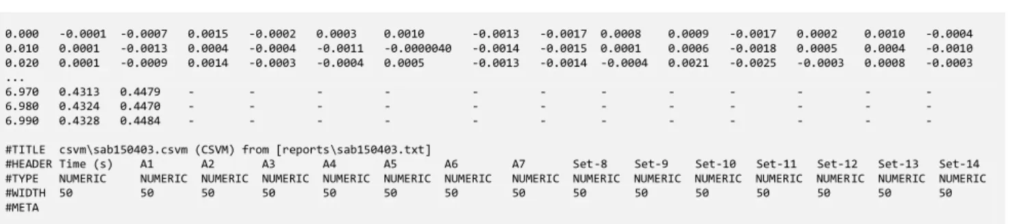
Figure 16-A. – A partial view of kinetics CSVM data, a lot of rows are not shown (marked by ‘…’ characters).
0.000 -0.0001 -0.0007 0.0015 -0.0002 0.0003 0.0010 -0.0013 -0.0017 0.0008 0.0009 -0.0017 0.0002 0.0010 -0.0004 0.010 0.0001 -0.0013 0.0004 -0.0004 -0.0011 -0.0000040 -0.0014 -0.0015 0.0001 0.0006 -0.0018 0.0005 0.0004 -0.0010 0.020 0.0001 -0.0009 0.0014 -0.0003 -0.0004 0.0005 -0.0013 -0.0014 -0.0004 0.0021 -0.0025 -0.0003 0.0008 -0.0003 ... 6.970 0.4313 0.4479 - - - - - - - - - - - - 6.980 0.4324 0.4470 - - - - - - - - - - - - 6.990 0.4328 0.4484 - - - - - - - - - - - -
#TITLE csvm\sab150403.csvm (CSVM) from [reports\sab150403.txt]
#HEADER Time (s) A1 A2 A3 A4 A5 A6 A7 Set-8 Set-9 Set-10 Set-11 Set-12 Set-13 Set-14 #TYPE NUMERIC NUMERIC NUMERIC NUMERIC NUMERIC NUMERIC NUMERIC NUMERIC NUMERIC NUMERIC NUMERIC NUMERIC NUMERIC NUMERIC NUMERIC #WIDTH 50 50 50 50 50 50 50 50 50 50 50 50 50 50 50 #META
This primary CSVM file can be generated de novo by users or acquisition system, but it can also result from another data format specific of a method or an apparatus. This was the case for this sample and the original format is shown in the following figure:
Figure 16-B. – Original format issued from a spectrophotometer..
X Y X Y X Y X Y --- 0.000 0.1112 0.050 0.1111 0.100 0.1111 0.150 0.1113 0.200 0.1116 0.250 0.0875 0.300 0.0514 0.350 0.0378 0.400 0.0696 0.450 0.1014 0.500 0.1126 0.550 0.1135 0.600 0.1145 0.650 0.1155 0.700 0.1164 0.750 0.1173 0.800 0.1181 0.850 0.1188 0.900 0.1194 0.950 0.1202 ...
This example show one interest of the CSVM format: to be used as a canonical data format for RAW tabular data. This permits to use data independently of the data source and in a better way than pure CSV files that cannot embed metadata and annotations.
29
S. Gavalda. L’Enolase de Trypanosoma brucei : Synthèse et étude du mode d’action d’inhibiteurs. Thèse de doctorat de l’Université Paul Sabatier Toulouse III (2005).
30
S. Gavalda, F. Rodriguez, G. Beyries, C. Blonski. Software design and components for enzymology,. 21ème CBSO, Ax-Les-Thermes (2006).
31
S. Gavalda, F. Rodriguez, G. Beyries, C. Blonski .Méthodes et composants logiciels pour l'interface chimie-biologie. RECOB11 Aussois (2006).
In the CSVM file shown in Figure 16-A, the amount of information seems to be low: the values of inhibitor concentration (#HEADER field) are tagged as A1, A2, … Set-14 which is not very explicit if the enzymologist wants to reuse the data later. In this case, the main information is the number of file: 150403 (date of experiment) stored in #TITLE field, this record number give access to another file with contains full information about experimental conditions.
This approach was used because we were not sure, at this time, if it was pertinent to store all parameters of the experiment with the data in the same CSVM file. It was possible to use the #META field for that, in another way the insertion of annotations in the CSVM table could be used 32.
Notice also that some of the last rows of this file are not filled with data. This is normal, all kinetics are not recorded with same duration (but with same time origin and intervals). The CSVM convention lets you to mark these empty positions by a particular character (in this case ‘-‘) or not.
5.2. Data extraction from RAW values
Very often calculation programs cannot handle multi-column files (not only CSVM) but uses a two-column file: time and a variation of a given quantity (here the product of reaction, for a particular value of inhibitor concentration). The following figure shows this kind of file with: a number of experimental points in the first row, followed by two columns using spaces as delimiters, one for time, the other for a biochemical quantity, and at last a block (rows beginning by a # character) for some metadata.
Figure 17. – A two-column data file specific of a given software. 691 0 0 0.05 0.67669 0.1 1.42857 0.15 2.18045 0.2 2.85714 ... 34.383 281.50376 34.433 281.8797 34.483 282.25564 # LPZ file . lpz\0234-1.lpz # Npts ... 691 ... # Colx no .. 0 # Header x . Time # Coly no .. 1 # Header y . B ...
In this case, we need to use software components to extract columns from the primary CSVM file, make this kind of dataset: {Time (s); A1}, {Time (s); A2} ... {Time(s); Set-14} and save it using the corresponding format. With CSVM it is easy to split the multi-column file (one time column, i=1..n columns [P]i) into n CSVM files (each on with time and [P]i). Column extractors are included in Python toolkit, a Python list is returned, depending on a search string applied on #HEADER values:
Code 4. – Simple CSVM column extractor in Python language.
print "*** Extract columns on the value of headers"
print "-> the column named 'fichier_mol' in strict mode (equal)" ls = csvm_ptr_getcol(c, 'fichier_mol', 1)
print "found %d column in CSVM stream" % (ls[0])
print ls[1]
print "-> the columns in which string 'no_' is found (include)" ls = csvm_ptr_getcol(c, 'no_', 0)
print "found %d columns in CSVM stream" % (ls[0])
32
And easy to do: if the first character of a row is a # not followed by a reserved keyword (TITLE, META, HEADER, TYPE or WIDTH) the row is not read by parsers and is available to store annotations, this kind of annotation provides a high level of
For large sets it is also possible to make queries based on all parts of CSVM (metadata and data) following the columns or rows. The following output shows on a simple string (green) matrix (the data block of a CSVM Python class) how to make a search or a combined search (AND, OR) on columns or rows:
Code 5. – Example of using a CSVM table for a file catalog (this output is a dump of a CSVM Python class).
*** Test EQ column queries samples
uses matrix : [['PDB', '3.24', 'AB4'], ['-', '1.0', '46'], ['PDB', '1.01', '4']]
query_col_eq(matrix, '4', 2, 1) => strict : rows [2]
query_col_eq(matrix, '4', 2, 0) => inc : rows [0, 1, 2]
query_col_eqs(matrix, 'PDB -', 'and', ' ', 0) => strict/and : rows []
query_col_eqs(matrix, 'PDB -', 'or', ' ', 0) => strict/or : rows [0, 2, 1]
query_col_eqs(matrix, '4 46', 'and', ' ', 2) => strict/and : rows []
query_col_eqsv(matrix, ['4','46'], 'or', 2) => strict/or : rows [2, 1]
query_col_eqsv(matrix, ['4','46'], 'or', 2, 0) => inc/or : rows [0, 1, 2]
*** Test NOT.EQ column queries samples
uses matrix : [['PDB', '3.24', 'AB4'], ['-', '1.0', '46'], ['PDB', '1.01', '4']]
query_col_not_eq(matrix, '4', 2) => strict : rows [0, 1]
query_col_not_eq(matrix, '4', 0, 0) => inc : rows [0, 1, 2]
query_col_not_eqs(matrix, '4 LIG', 'or', ' ', 0, 0) => inc : rows [0, 1, 2]
query_col_not_eqs(matrix, 'B 6', 'and', ' ', 2, 0) => inc : rows [2]
*** Test EQ row queries samples
get the first row of matrix : ['PDB', '3.24', 'AB4']
query_row_eq(row, '4') => strict : columns []
query_row_eq(row, '4', 0) => inc : columns [1, 2]
query_row_eqsv(row, ['4','PDB'], 'or', 0) => inc/or : columns [1, 2, 0]
*** Test NOT.EQ row queries samples
get the first row of matrix : ['PDB', '3.24', 'AB4']
query_row_not_eq(row, 'PDB') => strict : columns [1, 2]
query_row_not_eqs(row, 'B 4', 'and', ' ', 0) => inc/and : columns []
query_row_not_eqs(row, 'B 4', 'or', ' ', 0) => inc/or : columns [1, 0]
query_row_not_eqs(row, 'LIG -', 'or', ' ', 0) => inc/or : columns [0, 1, 2]
The results (red) of each tested functions (blue) are enclosed in brackets at right of lines. In strict mode the search string (or the list of search strings) must be found as a plain value of a cell, if not strict (in mode), the search string can be also a substring of a cell value.
With this minimal toolkit it is easy to extract columns or rows and to make files at a given format usable by software that cannot handle multi-column CSVM files. CSVM files and processors can simplify greatly the handling of complex dataflows.
5.3. Mixed time series and information
In this case, two column curves were extracted from the CSVM file (the primary data source) shown in Figure 16-A. Each extracted two-column files is formerly a curve [P]=f(t) and it can be used for calculation (curve fit). But what about for the results ? In the following sample, not only the results of minimization (data, model key, residuals) were stored in one CSVM file but also all parameters used for calculation (initial values, solution, confidence intervals …) by adding new columns at right of data.
The following output is a typical result after a calculation. The four first columns code for time series: column 1 for time (‘X0’), column 2 for product [P] concentration (‘Y0’), column 3 for curve fit using model C23 (‘Y0 CALC’) and column 4 for residuals (‘RES’) between experimental (Y0) and calculated (Y0 CALC) data.
Figure 18. – Results of a curve fitting calculation enclosed in a CSVM file.
0 0 0 0 LFILE A020304\LPZ\0234-17.LPZ .05 .97744 .6794984 .2979416 PROG Model C23 .1 1.8797 1.345653 .5340471 VER v:(1.0) .15 2.85714 1.998803 .8583375 NPTS 687 .2 3.83459 2.639278 1.195312 NPAR 3 .25 4.3609 3.267402 1.093498 NVAL 1 .3 4.66165 3.883489 .7781613 F 182.0163 .35 5.11278 4.487844 .6249361 ET .5158544 .4 5.86466 5.080766 .7838941 PNUM 1 .45 6.61654 5.662545 .9539948 PNAME k .5 7.21805 6.233466 .9845843 PSOL .5151757
.55 7.81955 6.793804 1.025746 PMIN .5145575 .6 8.42105 7.343827 1.077223 PMAX .5157939 .65 8.79699 7.883799 .9131913 PNUM 2 .7 9.24812 8.413976 .8341446 PNAME Vo .75 9.62406 8.934606 .6894541 PSOL 8.571785 .8 10.07519 9.445931 .6292582 PMIN 8.558927 .85 10.67669 9.94819 .7285004 PMAX 8.584643 .9 11.2782 10.44161 .8365898 PNUM 3 .95 11.65414 10.92642 .7277212 PNAME Vs 1 11.8797 11.40284 .4768639 PSOL 3.095204 1.05 12.10526 11.87107 .2341881 PMIN 3.092419 1.1 12.85714 12.33134 .5258017 PMAX 3.09799 1.15 13.60902 12.78383 .8251867 CNUM 1 1.2 14.13534 13.22876 .9065809 CNAME Quality 1.25 14.58647 13.6663 .920166 CVAL 991 1.3 15.03759 14.09666 .9409323 END - 1.45 16.01504 15.34638 .6686592 - - 1.5 16.39098 15.74975 .6412268 - - 1.55 16.69173 16.1468 .5449276 - - ... 34.183 125.4135 126.4381 -1.024567 - - 34.233 125.5639 126.5929 -1.028954 - - 34.283 125.8647 126.7476 -.8829575 - - # #TITLE / Model C23
#HEADER X0 Y0 Y0 calc RES KEY VALUE #TYPE NUMERIC NUMERIC NUMERIC NUMERIC TEXT NUMERIC #WIDTH 50 50 50 50 50 50 #META CSVM Result / VA04A QB BUILD
The two last columns are used to store calculation parameters and some results as a key-values scheme. This information are known as columns ‘KEY’, ‘VALUE’ and of type TEXT and NUMERIC and include primary data file (LFILE), program used (PROG), number of experimental points (NPTS), calculation values such as standard deviation (ET) and solution (PSOL) of model’s parameters (PNAME) with confidence intervals (PMIN, PMAX), or other post processing calculations (Quality).
The KEY-VALUE block is closed by a KEY=’END’, after this point the ‘KEY’ and ‘VALUE’ columns are filled with blank chars (‘-‘ in this case).
5.4. Combine different layers of data and calculations
This kind of file is considered a secondary data source, and these files could be aggregated to do other calculations. But, in fact, the most frequent use of secondary data is to pick some results inside (typically a solution value for a given parameter to be optimized). In this case, the value (PSOL=0.5151757) of an apparent kinetic constant k (PNUM=1, PNAME=k) was extracted, and stored in a new CSVM file: the
tertiary data source.
More precisely, this file was used to store the variation of k value (secondary data) with concentrations of [S] or [I] (substrate and inhibitor) stored in the primary data source (CSVM file shown in Figure 16). An example of tertiary data source is given in the Figure 19 :
Figure 19. – Aggregated results in a CSVM file and used as a new data source in the next calculation layer. Some columns are not shown and are marked by ’…’ symbols.
A020304 0234-1.LPZ Model C23 691 3 1 186.8595 .5211507 1 k ... A020304 0234-10.LPZ Model C23 686 3 1 224.6174 .5734709 1 k ... A020304 0234-11.LPZ Model C23 691 3 1 1373.348 1.41285 1 k ... A020304 0234-12.LPZ Model C23 690 3 1 152.6696 .4714091 1 k ... A020304 0234-13.LPZ Model C23 684 3 1 509.5747 .8650284 1 k ... ... TB310304 3134-8.LPZ Model C23 623 3 1 516.7548 .9129487 1 k ... TB310304 3134-9.LPZ Model C23 649 3 1 682.8931 1.028159 1 k ... #TITLE Results in [model_c23\][CSV]
#HEADER LFILE PROG NPTS NPAR NVAL F ET PNUM PNAME ... #TYPE UNDEF UNDEF UNDEF UNDEF UNDEF UNDEF UNDEF UNDEF UNDEF ... #WIDTH 50 50 50 50 50 50 50 50 50 ...
The tertiary data source was then used to make other calculations in order to compute an inhibition constant (KI or KI*) significant of the affinity of a given inhibitor relative to this enzyme and that is used to rank the efficiency of different inhibitors.
The details of equations used in this software pipe are given in Annex-1 with the same color conventions than in this section.
5.5. Data driven parallelism
This previous sample shows how CSVM could be used to follow closely data parallelism, the Figure 19 generalize this kind of concept:
Figure 20. – Data parallelism in the case of this Enzyme kinetics processing.
Experimental data Problem specification primary data Import Expansion (split) Curve fit Primary calculation Result files Secondary data Reduce (aggregate) Indexes and results
Tertiary data
Secondary calculations
Indexes and results Final report
The files in set j1 are native files (apparatus or other formats). These files (e4, e7 …) are converted to the canonical format in order to create a CSVM data space (e1, e2, e3 … e8). For each file of this space the n data sets (two-column sets time vs. quantity) are extracted, and n suitable files for calculation (CSVM or not depending on the software used) are created (i.e. m1 or m5 squares).
After calculation the results are stored in n CSVM files mixing original data and results (i.e. e4.1, e4.2, e4.3 … for columns m1, m2, m3 … of file e4).
Some data inside these files are then extracted and aggregated inside a new data source i1. This source can be used as a report or for a new calculation run. In this case a new file can be created or columns can be added to i1 that gives a modified i1.1
All calculations are independent and could be attributed to a pool of nodes/threads depending on the parallel model used. We can use CSVM as support for a data driven parallelism and it could be possible to implement an abstraction layer upon CSVM to make operations such as: split, scatter/bcast, reduce … (typically MPI-like operations on data at different calculation steps) in order to implement a model of high throughput enzymology. e2 e6 e5 e3 e1 e4 e4 e7 e8 m1 m1 m1 m1 m5 m5 m5
e4.1 e4.2 e4.3 e7.1 e7.2
i1 e4→e4.1.m1 e4→e4.2.m1 e4→e4.3.m1 … e7→e7.1.m5 e7→e7.2.m5 … s1 i1.1 e4→e4.1.m1→r1.4.1→... e4→e4.2.m1→r1.4.2→... e4→e4.3.m1→r1.4.3→... … j1 e4e7→→m5→m1→i1i1→→... …
5.6. From calculations to reports
In the previous sections we have shown that CSVM is well suited to support publication chains. This also the case here, the final (i.e. i1.1) or intermediate reports (i1) can be used as input for a new dataflow (calculation or data exposition). The following figure shows a proof of concept for a report layer at the level i1 that includes a JavaScript framework and software components for extracting data (i.e. make graphs) from the CSVM files.
5.7. Including models in the scheme
Calculations uses a phenomenological model for data fitting, now what about the model itself ? The following sample shows how a model could be stored 33 in a CSVM table. The chosen model is very used in enzyme kinetics: a variation of Michaelis-Menten mechanism that is converted as an EDO system and stored with all needed parameters for numerical integration inside a CSVM table using a key/values scheme.
A model taken from enzymology : Converted in a EDO system : The corresponding CSVM file shown in the following figure includes other equations (mass conservation, enzyme conservation), values for rate constants and molar concentrations, integration algorithm used (in this case RK4 stands for Runge-Kutta 4) and its parameters, other non-numerical data …
Figure 22. – EDO system and parameters stored in a CSVM file (human readable form).
ALGO rk4 - - - EDO solver TIME 0 1 0.0000001 0.01 Seconds
SPEC S 1.0e-3 - - Substrat (M, publi= 10.10-6) SPEC P 0.0 - - Product (M)
SPEC ES 0.0 - - Enzyme-substrat complex (M)
SPEC E 1.0e-006 - - Free Enzyme (M, publi= 45.5 10-12 M) RATE k1 2.0e+005 - - ct. ES formation (M-1.s-1)
RATE k-1 1.1e+003 - - ct. ES disparition (s-1) RATE k2 900 - - ct. P formation (s-1) # Theoric KM of 10.10-3 M
PATH S <k -1>.ES - <k1>.E.S - - dS/dt PATH P <k2>.ES - - dP/dt PATH ES <k1>.E.S - <k -1>.ES - <k2>.ES - - dES/dt PATH E - <k1>.E.S + <k -1>.ES + <k2>.ES - - dE/dt
MONI Cm S+P+ES+E - - Matter conservation MONI Etotal E+ES - - Enzyme conservation
#TITLE Prob 3.3 of Shuler and Kargi S>>E
#HEADER KEY UNDEF UNDEF UNDEF UNDEF UNDEF #TYPE TEXT TEXT TEXT TEXT TEXT TEXT #WIDTH 50 50 50 50 50 50
This is a proposal for coding the model in order to ensure genericity (a same formalism is usable for all models) and to keep human readable data (a formalism closely related to EDO system). Perhaps it is not the best solution for presenting data closely from the syntax and calling arguments of the numerical function used to make numerical integration. But in two cases, the CSVM file will be easily parsed independently of model’s complexity, and a one problem will be eliminated.
Similar examples could be found in chemistry, environmental sciences, etc. In these cases, CSVM shows that it is possible to store in the same format, the data and intermediate data, the results, the models. This is useful in a lot of experimental sciences because the development effort for computer scientists is reduced and they can focus on the problem itself.
33 Stored and parsed. We have used this approach for simulation, not for modeling because we use mainly analytical solutions rather than numerical solutions in our work.
6. Limit the number of data formats you use!
We have spoken about the use of CSVM as a canonical format for RAW data conversion and intermediate results. Extending the concept to other kind of data is fairly immediate. In this section some samples taken from structural bioinformatics are given.
6.1. Map of molecular interactions
The previous section has shown that CSVM can be used to store results of calculations. This ensures that these results could be used by another program or could be aggregated to larger dataset without any modifications. This is also true for non-time dependant data, here is a case for a map of molar interaction between a ligand (COA standing for Coenzyme A) and the water (HOH) or amino acid residues (LYS, ARG, ALA, SER, …) of an enzyme (1KRU PDB structure), courtesy from Vincent Mariaule 34
.
A software pipe generates a custom 2D map of interaction using different programs: LIGPLOT 35 package and related programs 36 37, the results of different calculations are filtered, extracted, converted and aggregated in the final CSVM file.
Figure 23. – A 2 D interaction map stored as a CSVM table.
1KRU 1KRU LYS 195 N d HOH 2053 O a 2.83 1KRU 1KRU COA 204 S1P d IPT 207 O6 a 3.14 1KRU 1KRU HOH 2053 O d COA 204 O4A a 2.92 1KRU 1KRU COA 204 OAP d COA 204 N7A a 2.52 1KRU 1KRU ARG 183 NH2 d COA 204 O5A a 3.09 1KRU 1KRU ARG 183 NE d COA 204 O5A a 3.22 1KRU 1KRU COA 204 N6A d ALA 160 O a 2.95 1KRU 1KRU ALA 160 N d COA 204 O9P a 3.16 1KRU 1KRU SER 142 N d COA 204 O5P a 2.81 1KRU 1KRU IPT 207 C6 - COA 204 S1P - 3.60 1KRU 1KRU COA 204 C2A - VAL 177 CG1 - 3.84 1KRU 1KRU COA 204 S1P - HIS 115 CD2 - 3.48 1KRU 1KRU COA 204 C6A - ALA 175 CB - 3.89 1KRU 1KRU COA 204 C7P - TRP 139 CH2 - 3.76 1KRU 1KRU COA 204 CEP - TRP 139 CH2 - 3.65 1KRU 1KRU COA 204 CEP - TRP 139 CZ3 - 3.60 1KRU 1KRU COA 204 C6P - TRP 139 CZ2 - 3.74 1KRU 1KRU COA 204 C7P - TRP 139 CZ2 - 3.57 1KRU 1KRU COA 204 C3P - ALA 105 CB - 3.45
#TITLE Ligplot summary!ligplot2csvm.py (v:1.04)!1KRU
#HEADER PDB CHAIN RESNAME RESSEQ ATYPE FROM RESNAME RESSEQ ATYPE TO DIST #TYPE TEXT TEXT TEXT INTEGER TEXT TEXT TEXT INTEGER TEXT TEXT FLOAT #WIDTH 10 10 10 10 10 10 10 10 10 10 10
The d and a acronyms stands for donor and acceptor (hydrogen interactions), the columns RESSEQ are used to store the residue number in the protein sequence or in the crystallographic structure. The columns ATYPE store the atom types implied in interactions. The formalism is closely related to the Protein Data Bank 38 (PDB) formalism. The last column is the distance between the two atoms found by row.
Is structural data (a PDB 39 file) or sequence data could be stored in CSVM files ? Definitely yes, but the interest could be limited because a lot of file formats exists and are widely used.
34
V. Mariaule. Etude structurale des histones acétyl transférases. Rapport M1 BBT, Université Paul Sabatier Toulouse III (2008).
35
A.C. Wallace, R.A. Laskowski, J.M. Thornton. LIGPLOT: a program to generate schematic diagrams of protein-ligand interactions. Protein Eng. (1995) 8:2, 127-134.
36
HBPLUS: Hydrogen Bond Calculation Program - I.K. McDonald, J.M. Thornton. Satisfying Hydrogen Bonding Potential in Proteins (1994) JMB 238, 777-793.
37
NACCESS: Solvent accessible area calculations – S. Hubbard, J. Thornton (1992).
38
RCSB Protein Data Bank - http://www.rcsb.org/pdb/
39
In the case of a PDB file, the coordinates PDB block is immediately transposable, in the case of CSVM the use of delimiters permits to add new columns in any order and to add useful annotations. For the header PDB block using CSVM could simplify the metadata organization because CSVM is not restricted to a particular number of columns or characters per row. Sometimes, for intermediate results in calculations or protein coordinate normalization we had used CSVM for coordinate
6.2. BLOSSUM and PAM matrixes
For people working in genomics or proteomics, BLOSUM or PAM substitution matrixes 40 are well known objects. The next figure shows a CSVM version of a BLOSSUM 62 matrix. For readability, some columns of the metadata block are missing (and marked by ‘…’ characters at right).
The order of amino acid names (1-letter code in #HEADER) is the same in columns (left to right) and rows (top to bottom), data taken from Hiroto Saigo 41.
Figure 24. – A Blossum 62 matrix encoded in a CSVM table.
4 - - - - -1 5 - - - - -2 0 6 - - - - -2 -2 1 6 - - - - 0 -3 -3 -3 9 - - - - -1 1 0 0 -3 5 - - - - -1 0 0 2 -4 2 5 - - - - 0 -2 0 -1 -3 -2 -2 6 - - - - -2 0 1 -1 -3 0 0 -2 8 - - - - -1 -3 -3 -3 -1 -3 -3 -4 -3 4 - - - - -1 -2 -3 -4 -1 -2 -3 -4 -3 2 4 - - - - -1 2 0 -1 -3 1 1 -2 -1 -3 -2 5 - - - - -1 -1 -2 -3 -1 0 -2 -3 -2 1 2 -1 5 - - - - -2 -3 -3 -3 -2 -3 -3 -3 -1 0 0 -3 0 6 - - - - -1 -2 -2 -1 -3 -1 -1 -2 -2 -3 -3 -1 -2 -4 7 - - - - - 1 -1 1 0 -1 0 0 0 -1 -2 -2 0 -1 -2 -1 4 - - - - 0 -1 0 -1 -1 -1 -1 -2 -2 -1 -1 -1 -1 -2 -1 1 5 - - - -3 -3 -4 -4 -2 -2 -3 -2 -2 -3 -2 -3 -1 1 -4 -3 -2 11 - - -2 -2 -2 -3 -2 -1 -2 -3 2 -1 -1 -2 -1 3 -3 -2 -2 2 7 - 0 -3 -3 -3 -1 -2 -2 -3 -3 3 1 -2 1 -1 -2 -2 0 -3 -1 4 #TITLE BLOSSUM62 #HEADER A R N D C Q E G H I ... #TYPE NUMERIC NUMERIC NUMERIC NUMERIC NUMERIC NUMERIC NUMERIC NUMERIC NUMERIC NUMERIC ... #WIDTH 10 10 10 10 10 10 10 10 10 10 ... #META from http://sunflower.kuicr.kyoto-u.ac.jp/~hiroto/project/optaa.html
Using same and unified file format for different parameters sets is interesting to minimize error and developments. Standard or reference data/charts are used in a lot of scientific fields, and it could be useful to take advantage from a canonical and generic format.
6.3. PDB hetero compound dictionary and variations
The following figure shows the bottom of the PDB’s databank hetero dictionary 42 encoded in CSVM. This file of about 2000 rows, is used to store PDB and chemical component identifier correspondences.
In example, the chemical component encoded with name ZZM (1-propan-2-yl-3-(2-pyridin-3-ylethynyl)pyrazolo[4,5-e]pyrimidin-4-amine) is found in PDB structure 2WXM (phosphoinositide-3-OH kinase). So, the first column is for the chemical compound PDB code (3 chars) and the column 2 is for a list (values separated by a space) of PDB entries (4 chars) in which the compound is found.
The CSVM format is not locked to tabular data of a given number of columns, formerly the following table is constituted of two columns (HETNAME, INPDB) but in the second column, the values could be single (last lines shown) or multiple (first line with 3 values: 2wtv, 2wtw, 2x81).
It is possible to make 3 columns to store these values, but if the average amount of values by line is near 1, you will have a lot of unused columns needed by lines in which the number of values is high. This is precisely the case in this example; and it is better to define lines with two columns and to use a secondary delimiter in the INPDB column. Here a ‘ ‘ (space) character is used, but another could be used, the best in this case is a character 43 not found in current scientific data.
40
Substitution matrix (Wikipedia) - http://en.wikipedia.org/wiki/Substitution_matrix
41
Akutsu Laboratory - http://sunflower.kuicr.kyoto-u.ac.jp/index.html.en
42
Ligand Expo Downloads - http://ligand-expo.rcsb.org/ld-download.html
43
The CSVM parser split the file according to the main delimiter (generally a TAB) and the application program, read CSVM matrix cells and split them knowing the secondary (or ternary) delimiter, if multiple values are expectable inside.
The CSVM formalism allows to send a signal through the parser about that (multiple values in cells). The #META row could be used with a specific keyword inside (the signal and the secondary delimiter), in example: ‘#META MULTIPLE_VALUES_IN_CELLS[§] …’ or ‘#META CODE104 CODE108 …’ etc. This signal can be interpreted (post-parsing) by the application layer. As usual we don’t define in CSVM specification this kind of mechanism; the interest of CSVM is precisely to provide architecture for data and metadata but without any normalization.
Figure 25. – PDB and chemical component identifier (column HETNAME) correspondences encoded in a CSVM file.
... ZZL 2wtv 2wtw 2x81 ZZM 2wxm ZZN 2wxg ... ZZU 2wbp 2wbq ZZY 2wd1 ZZZ 2cfi #TITLE cc-to-pdb.tdd #HEADER HETNAME INPDB #TYPE TEXT TEXT #WIDTH 10 10
#META http://ligand-expo.rcsb.org/ld-download.html|20jul2010
In this sample the #META field is used to store the download location, and a release date (using another delimiter the ‘|’ character). The CSVM format let the user free from defining characters used as primary or secondary delimiters, both for data or metadata block, the parser knows only column delimiter, others separators are used by application.
Real case: how to merge CSVM tables
The previous file (Figure 25) is very close from original file (the dictionary released by the PDB): only a metadata block has been added. This is also the case for the next file (Figure 26): another dictionary taken from the PDB listing the same hetero compounds with the same 3 letter code (column HETNAME) and two other columns for a chemical formula written in SMILES format (SMI column) and a chemical name (MOLNAME):
Figure 26. – Last rows of a SMILES data file including PDB chemical component identifier (column HETNAME).
...
C(CNC(=N)N)C(C(C(=O)O)N)O ZZU (2s,3s)-hydroxyarginine
c1ccc(c(c1)[N+](=O)[O-])S(=O)(=O)n2ccc3c2cc(cn3)C(=O)N ZZY 1-[(2-nitrophenyl)sulfonyl]-1h-pyrrolo[3,2-b]pyridine-6-carboxamide
C1C(NC2=C(N1)N=C(NC2=O)N)C=O ZZZ 6-formyltetrahydropterin
#TITLE Components-smiles-oe.smi #HEADER SMI HETNAME MOLNAME #TYPE TEXT TEXT TEXT #WIDTH 10 10 10
#META http://ligand-expo.rcsb.org/ld-download.html|20jul2010
Even if the only modifications were to add a metadata block, this enables complex operations such as the merging of the files from Figure 25 and of Figure 26. This can be done with a few lines of code and functions from the Python CSVM toolkit. This example is given in the following and it will be used to illustrate some subtleties related to the manipulation of RAW data sets.
![Figure 2. –A view of the collection written in a table, only rows [1..10] and [78..80] are shown](https://thumb-eu.123doks.com/thumbv2/123doknet/13507028.415705/3.892.75.831.835.1032/figure-view-collection-written-table-rows-shown.webp)